ECE-320: Linear Control Systems Homework 9
Due: Friday May 14 at the (very) beginning of lab
In this homework we will simulate and study integral control, full order observers coupled with state variable feedback, and then we will combine them. Having an integrator in our system is generally preferable to using a prefilter for achieving a zero steady state error for a step input, since it will help overcome errors in the plant model. Some of the things we will do in this homework are a bit weird, but they are being done for the sake of demonstrating that your programs are working.
For all of these problems, use the state models available on the class website. Both systems are torsional systems.
Be sure you are using a variable step solver, and the maximum time step is something like 1e-5 (look under Simulation-> Configuration Parameters). Also, set the initial conditions on the integrators to just 0 (a scalar).
Some useful Matlab commands are
[n,m] = size(A); zeros(n,m); eye(n)
You need to save plots of every case you are told to run. Save them in a word document with appropriate figure captions and turn that in (or e-mail it). This entire homework is a pre-lab.
1) In this problem we will incorporate integral control for a one degree of freedom system and run some test cases to verify your code is working.
a) Copy your program Basic_1dof_State_Variable_Model_driver.m to a new file
[image:1.612.72.522.558.678.2]sv1_integral_driver.m, then copy the Simulink file Basic_1dof_State_Variable_Model.mdl to sv1_integral.mdl. Modify these new files to implement state variable feedback using integral control. The basic integral control scheme is shown below in Figure 1. Note that the prefilter is equal to 1.
b) Modify sv1_integral_driver.m to plot the two states and the control effort (the control
) Set the step amplitude to 10 degrees (but convert to radians), the final time to 1.5 seconds,
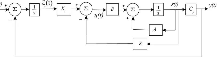
Figure 2. Initial results for the 1 dof system with integral control (problem 1c).
) At this point there is no real reason for us to use integral control, since we know everything
tion,
erything
) Systems with these integrators have an interesting characteristic. Change the poles to 5,
-remove the line A = A*0.25, or you will have trouble in lab! effort does not get scaled to degrees).
c
place the poles at -5, -10, -15, and run the simulation. You should get results like those shown in Figure 2.
0 0.5 1 1.5
0 5 10
D
isk
P
o
si
ti
o
n
(
d
e
g
)
0 0.5 1 1.5
0 10 20 30
D
is
k
Ve
lo
ci
ty
(d
e
g
/s
e
c
)
0 0.5 1 1.5
0 0.02 0.04 0.06 0.08
C
o
nt
rol
E
ff
o
rt
d
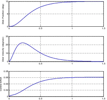
exactly. Let’s assume your lab partner is way off on the system model. In your code, just before your run the simulation (just before the sim command), type A = A*0.25, which basically says you’re a matrix is way off. If you make this change just before the simula your gains will be chosen assuming your model is correct, and we will be running the simulation using a different system. Change the final time to 2.5 seconds, and leave ev
else the same as before. You should get results like those shown in Figure 3, which look pretty hopeless, but we can improve them.
e
[image:2.612.119.467.157.483.2]Figure 3. Integral control of a 1 dof system with bad data (problem 1d)
0 0.5 1 1.5 2 2.5
0 5 10 15 20
D
is
k
Po
s
iti
o
n
(
d
e
g
)
200
D
is
k
Ve
lo
c
ity
(
d
e
g
/s
e
c
)
100
0
-100
0 0.5 1 1.5 2 2.5
0.03
0 0.5 1 1.5 2 2.5
0 0.01 0.02
Co
n
tro
l E
ff
o
rt
0 0.5 1 1.5 2 2.5
0 5 10 15
D
is
k
P
o
s
it
ion (
d
eg)
0 0.5 1 1.5 2 2.5
-50 0 50 100
D
is
k
Ve
lo
c
ity
(
d
e
g
/s
e
c
)
0 0.5 1 1.5 2 2.5
0 0.005 0.01 0.015 0.02
Con
tro
l E
ff
o
Figure 4. Integral control of a 1 dof system with bad data, but a better result (problem 1e). 2)
n some test cases to verify your code is working.
_Model_driver.m to a new file
v2_integral_driver.m, then copy the Simulink file Basic_2dof_State_Variable_Model.mdl In this problem we will incorporate integral control for a two degree of freedom system and ru
a) Copy your program Basic_2dof_State_Variable s
to sv2_integral.mdl. Modify these new files to implement state variable feedback us integral control.
b) Modify sv2_in
ing
tegral_driver.m to plot the four states and the control effort (the control ffort does not get scaled to degrees).
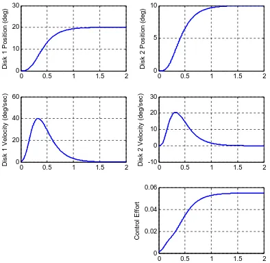
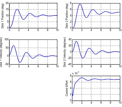
final time to 2 seconds, and place the poles at 5, 10, -5, -20, -25. We are trying to control the position of the second disk. Run the simulation and
Figure 5. Integral control of a two degree of freedom system. We care controlling the position of the second disk (part 2c).
e
c) Set the amplitude to 10 degrees, the 1
you should get results like those shown in Figure 5.
0 0.5 1 1.5 2
0 10 20
30 10
D
is
k
1
P
os
it
ion
(deg
)
0 0.5 1 1.5 2
0 20 40 60
D
is
k
1
V
e
lo
c
ity
(
d
e
g
/s
e
c
)
0 0.5 1 1.5 2
0 5
D
is
k
2
P
os
it
ion
(deg
)
30
D
is
k
2
V
e
lo
c
ity
(
d
e
g
/s
e
c
)
20
10
0
-10
0 0.5 1 1.5 2
0.06
0 0.5 1 1.5 2
0 0.02 0.04
Co
n
tro
l E
ff
o
[image:4.612.96.490.300.683.2]d) Assume your lab partner screwed up gain, so you model is not accurate. To see what appens when the model does not match the real system, just before the simulation type A =
, you
igure 6. Integral control of a 2 dof system with bad data. We are controlling the position of e second disk (problem 2d).
e same as in part d, but now we want to control the position of e first disk. You should get results like those in Figure 7. If your results agree, remove the h
A*0.25, place the poles at -5, -10, -15, -20, -2500, and run the simulation for 10 seconds should get a plot like that in Figure 6.
0 2 4 6 8 10
0 10 20 30
40 20
F th
e) Now assume everything is th th
line A = A*0.25 from your code.
D
is
k
1
P
os
it
io
n (
d
eg)
0 2 4 6 8 10
-100 0 100 200
D
isk 1
V
e
lo
ci
ty (
d
e
g
/se
c)
0 2 4 6 8 10
0 5 10 15
D
is
k
2
P
os
it
io
n (
d
eg)
D
isk 2
V
e
lo
ci
ty (
d
e
g
/se
c) 100
50
0
-50
0 2 4 6 8 10
0.015
0 2 4 6 8 10
0 0.005 0.01
C
o
n
tro
l E
ff
o
Figure 7. Integral control of a 2 dof system with bad data. We are controlling the position of the first disk (problem 2e).
0 2 4 6 8 10
0 5 10 15 20
D
is
k
1 P
os
it
ion (
d
eg)
0 2 4 6 8 10
-50 0 50 100
D
is
k
1
V
el
oc
it
y
(
deg/
s
ec
)
0 2 4 6 8 10
0 2 4 6 8
D
is
k
2 P
os
it
ion (
d
eg)
0 2 4 6 8 10
-40 -20 0 20 40
D
is
k
2
V
el
oc
it
y
(
deg/
s
ec
)
0 2 4 6 8 10
0 2 4 6
8x 10
-3
Co
n
tro
l E
ff
o
3) In this problem we will incorporate a full order observer for a one degree of freedom system and run some test cases to verify your code is working.
a) Copy your program Basic_1dof_State_Variable_Model_driver.m to a new file sv1_observer_driver.m, then copy the Simulink file
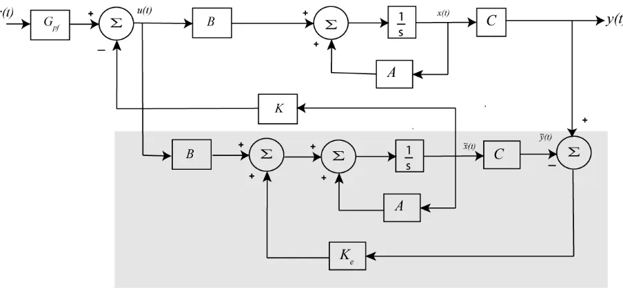
[image:7.612.66.518.199.410.2]Basic_1dof_State_Variable_Model.mdl to sv1_observer.mdl. Modify these new files to implement state variable feedback using integral control. The basic integral control scheme is shown below in Figure 8.
Figure 8. Full order observer state variable feedback structure.
b) Modify sv1_observer_driver.m to plot the each of the true and estimated states on the same graph. See Figure 9 (or Figure 10) for an example.
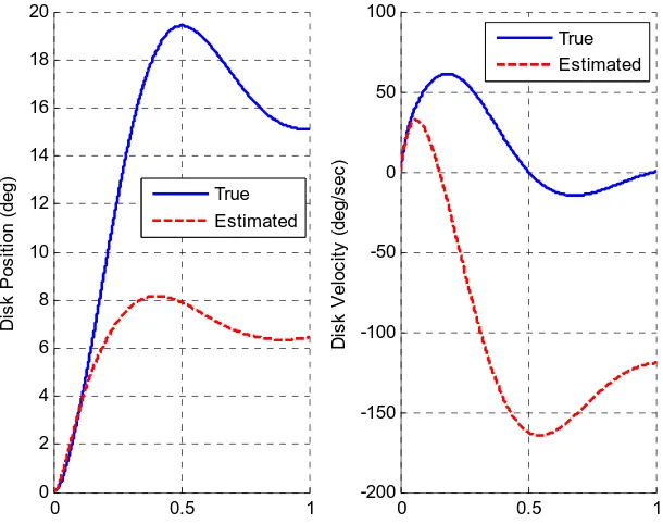
c) For an input of 10 degrees, a final time of 1 second, and both the state feedback and observer poles at p = [-10 -12], you should get a graph like that in Figure 9.
d) Now we will try and observe what happens when there is a difference between our model and the real system. Modify the observer subsystem in the model (.mdl) file, so the A matrix in the observer is called AA. Just before theyou run the model file, enter the command AA = A*1.5. You should get results like those in Figure 10.
Figure 9. Results for full order observer for 1 dof system (problem 3c).
0 0.5 1
0 1 2 3 4 5 6 7 8 9 10
D
is
k
Po
s
iti
o
n
(
d
e
g
)
True Estimated
0 0.5 1
0 5 10 15 20 25 30 35 40 45
D
is
k
Ve
lo
c
ity
(
d
e
g
/s
e
c
)
True Estimated
0 0.5 1
0 2 4 6 8 10 12 14 16 18 20
D
is
k
Po
s
iti
o
n
(
d
e
g
)
True Estimated
0 0.5 1
-200 -150 -100 -50 0 50 100
D
is
k
Ve
lo
c
ity
(
d
e
g
/s
e
c
)
True Estimated
[image:8.612.138.452.71.310.2] [image:8.612.140.445.353.594.2]0 0.5 1 0
5 10 15 20 25
D
is
k
Po
s
iti
o
n
(
d
e
g
)
True Estimated
0 0.5 1
-100 -80 -60 -40 -20 0 20 40 60
D
is
k
Ve
lo
c
ity
(
d
e
g
/s
e
c
)
[image:9.612.140.446.71.311.2]True Estimated
Figure 11. Results for the 1dof full order observer for a significant model error (problem 3e).
Figure 12. Results for the 1dof full order observer for a significant model error (problem 3e).
0 0.5 1
0 5 10 15
D
is
k
Po
s
iti
o
n
(
d
e
g
) True
Estimated
0 0.5 1
-30 -20 -10 0 10 20 30 40 50 60
D
is
k
Ve
lo
c
ity
(
d
e
g
/s
e
c
)
[image:9.612.137.451.353.592.2]4) In this problem we will incorporate a full order observer for a two degree of freedom system and run some test cases to verify your code is working. You may need to include a vector Cy to correctly set the prefilter gain for the disk you are trying to control.
a) Copy your program Basic_2dof_State_Variable_Model_driver.m to a new file sv2_observer_driver.m, then copy the Simulink file
Basic_2dof_State_Variable_Model.mdl to sv2_observer.mdl. Modify these new files to implement state variable feedback using integral control.
b) Modify sv2_observer_driver.m to plot the each of the true and estimated states on the same graph. See Figure 13 for an example.
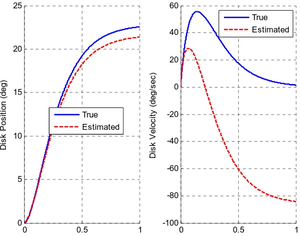
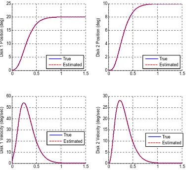
[image:10.612.103.479.305.649.2]c) For an input of 10 degrees, a final time of 1.5 second, and both the state feedback and observer poles at p = [-10, -12, -14, -16], controlling the position of the second disk with the input to the observer the position of the second disk, you should get a graph like that in Figure 13.
Figure 13. Full order observer for a 2 dof system (problem 4c).
0 0.5 1 1.5
0 5 10 15 20 25
D
is
k
1 P
o
s
it
ion (
d
eg)
True Estimated
0 0.5 1 1.5
0 10 20 30 40 50 60
D
is
k
1 V
e
loc
it
y
(
d
eg/
s
ec
)
True Estimated
0 0.5 1 1.5
0 2 4 6 8 10
D
is
k
2 P
o
s
it
ion (
d
eg)
True Estimated
0 0.5 1 1.5
0 5 10 15 20 25 30
D
is
k
2 V
e
loc
it
y
(
d
eg/
s
ec
)
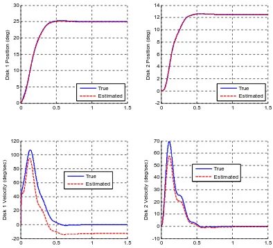
d) Now we will try and observe what happens when there is a difference between our model and the real system. Modify the observer system in the model (.mdl) file, so the A matrix is called AA. Just before you run the model file, enter the command AA = A*1.2. Place the state feedback poles at twice their original values (at 2*p), and change the observer poles to be ten times their original values (10*p). You should get results like those in Figure 14. Note that if we do not change the pole locations, we will get an unstable system (just try it!)
Figure 14. Full order observer for a 2 dof system with a bad model (problem 4d).
0 0.5 1 1.5
0 5 10 15 20 25 30
D
is
k
1
P
o
s
it
ion (deg)
True Estimated
0 0.5 1 1.5
-20 0 20 40 60 80 100 120
D
isk 1
V
e
lo
ci
ty
(
d
e
g
/se
c)
True Estimated
0 0.5 1 1.5
-2 0 2 4 6 8 10 12 14
D
is
k
2
P
o
s
it
ion (deg)
True Estimated
0 0.5 1 1.5
-10 0 10 20 30 40 50 60 70
D
isk 2
V
e
lo
ci
ty
(
d
e
g
/se
c)
True Estimated
e) Now rerun the system assuming the input to the observer is the position of the first and second disk, keeping everything else the same as in part d. You should the results like those in Figure 15.
f) Now rerun the system with the following changes, AA = 0.8*A. The input to the observer is still the position of the first and second disk. You should get results like those in Figure 16.
Figure 15. Full order observer for a 2 dof system with a bad model (problem 4e).
0 0.5 1 1.5
0 5 10 15 20 25 D is k 1 P os it ion ( deg ) True Estimated
0 0.5 1 1.5
-20 0 20 40 60 80 100 120 D is k 1 V el oc it y ( deg/ s ec ) True Estimated
0 0.5 1 1.5
-2 0 2 4 6 8 10 12 D is k 2 P os it ion ( deg ) True Estimated
0 0.5 1 1.5
-10 0 10 20 30 40 50 60 70 D is k 2 V el oc it y ( deg/ s ec ) True Estimated
Figure 16. Full order observer for a 2 dof system with a bad model (problem 4f).
0 0.5 1 1.5
0 2 4 6 8 10 Di s k 1 P o s it ion (d eg ) True Estimated
0 0.5 1 1.5
0 10 20 30 40 50 60 D is k 1 V el oc it y ( deg/ s ec ) True Estimated
0 0.5 1 1.5
-1 0 1 2 3 4 5 Di s k 2 P o s it ion (d eg ) True Estimated
0 0.5 1 1.5
[image:12.612.104.479.70.689.2]5) In this problem we will incorporate a full order observer and an integrator for a one degree of freedom system and run some test cases to verify your code is working.
a) Copy your program sv1_observer_driver.m to a new file sv1_observer_int_driver.m, then copy the Simulink file sv1_observer.mdl to sv1_observer_int.mdl. Modify these new
[image:13.612.67.523.182.357.2]files to implement state variable feedback with an observer using integral control. The basic control scheme is shown below in Figure 17.
Figure 17. Full order observer state variable feedback structure with integral control. b) For an input of 10 degrees, a final time of 1 second, place the state feedback poles at ps = [ -35, -20+10j, -20-10j] and observer poles at po = [-25 -30], you should get a graph like that in Figure 18.
0 0.5 1
0 2 4 6 8 10 12
D
isk
P
o
si
ti
o
n
(
d
e
g
) TrueEstimated
0 0.5 1
-10 0 10 20 30 40 50 60 70 80
D
isk
V
e
lo
c
ity (
d
e
g
/s
e
c
)
True Estimated
[image:13.612.152.437.439.659.2]c) Now we will try and observe what happens when there is a difference between our model and the real system. Modify the observer block in the model file, so the A matrix is called AA. Just before the you run the model file, enter the command AA = A*1.5. You should get results like those in Figure 19.
0 0.5 1
0 2 4 6 8 10 12 14
D
isk
P
o
si
ti
o
n
(
d
e
g
)
True Estimated
0 0.5 1
-150 -100 -50 0 50 100
D
is
k V
e
lo
ci
ty (
d
e
g
/s
e
c
)
True Estimated
Figure 19. Full order observer with integrator and bad data (problem 5c).
d) Now change the observer poles so they are 10 larger than before (10*po). You should get results like those in Figure 20.
Figure 20. Full order observer with integrator and bad data (problem 5d).
0 0.5 1
0 1 2 3 4 5 6 7 8 9 10
D
isk
P
o
si
ti
o
n
(
d
e
g
)
True Estimated
0 0.5 1
-10 0 10 20 30 40 50 60 70 80 90
D
is
k V
e
lo
ci
ty (
d
e
g
/s
e
c
)
[image:14.612.140.438.135.365.2] [image:14.612.146.444.455.683.2]Note that in both Figures 19 and 20, the steady state error is zero, even if the observer is not converged.
6) In this problem we will incorporate a full order observer and an integrator for a two degree of freedom system and run some test cases to verify your code is working. You may need to include a vector Cy to correctly set the prefilter gain for the disk you are trying to control.
a) Copy your program sv2_observer_driver.m to a new file sv2_observer_int_driver.m, then copy the Simulink file sv2_observer.mdl to sv2_observer_int.mdl. Modify these new
files to implement state variable feedback with an observer using integral control.
b) For an input of 10 degrees, a final time of 1 second, both the state feedback poles at ps = [-10, -12, -14, -16, -18], the observer poles at po = [-10 -12 -14 -16], the output of the system is the position of the second disk and the input to the observer is the position of both disks, you should get a graph like that in Figure 21.
Figure 21. State feedback, full order observer, and integral control for the 2 dof system (problem 6b).
0 0.5 1 1.5 2
0 5 10 15 20 25
D
is
k
1
P
o
s
it
ion
(de
g)
True Estimated
0 0.5 1 1.5 2
0 10 20 30 40 50 60
D
isk
1
V
e
lo
ci
ty (
d
e
g
/s
e
c)
True Estimated
0 0.5 1 1.5 2
0 2 4 6 8 10
D
is
k
2
P
o
s
it
ion
(de
g)
True Estimated
0 0.5 1 1.5 2
-10 0 10 20 30
D
isk
2
V
e
lo
ci
ty (
d
e
g
/s
e
c)
True Estimated
[image:15.612.123.460.314.593.2]d) Now change the observer poles to be 10 times larger than before (10*po). You should get the figure like that in Figure 23.
e) Rerun the same case as in part d, but now use AA = 0.5*A and the output is the position of the first disk. You should get results like those in Figure 24.
f) Rerun the same case as in part e, but now make the state feedback poles twice as large as they originally were (2*ps, leave the observer poles where they are). You should get results like those in Figure 25.
0 0.5 1 1.5 2
-10 0 10 20 30 40 50
D
is
k
1 P
o
s
it
ion
(de
g
)
True Estimated
0 0.5 1 1.5 2
-300 -200 -100 0 100 200
D
isk 1
V
e
lo
ci
ty
(
d
e
g
/se
c)
True Estimated
0 0.5 1 1.5 2
-5 0 5 10 15 20 25
D
is
k
2 P
o
s
it
ion
(de
g
)
True Estimated
0 0.5 1 1.5 2
-150 -100 -50 0 50 100
D
isk 2
V
e
lo
ci
ty
(
d
e
g
/se
c)
[image:16.612.112.471.233.515.2]True Estimated
Figure 23. State feedback, full order observer, and integral control for the 2 dof system with a bad model (problem 6d).
0 0.5 1 1.5 2
0 5 10 15 20 25 D is k 1 P os it io n ( d eg) True Estimated
0 0.5 1 1.5 2
-20 0 20 40 60 80 D isk 1 V e lo ci ty ( d e g /s e c) True Estimated
0 0.5 1 1.5 2
-5 0 5 10 15 D is k 2 P os it io n ( d eg) True Estimated
0 0.5 1 1.5 2
-10 0 10 20 30 40 D isk 2 V e lo ci ty ( d e g /s e c) True Estimated
Figure 24. State feedback, full order observer, and integral control for the 2 dof system with a
0 0.5 1 1.5 2
0 2 4 6 8 10 D is k 1 P os it io n (deg) True Estimated
0 0.5 1 1.5 2
0 10 20 30 40 D isk 1 V e lo ci ty ( d e g /s e c ) True Estimated
0 0.5 1 1.5 2
-2 0 2 4 6 D is k 2 P os it io n (deg) True Estimated
0 0.5 1 1.5 2
[image:17.612.113.481.84.380.2] [image:17.612.125.458.424.681.2]Figure 25. State feedback, full order observer, and integral control for the 2 dof system with a bad model (problem 6f).
0 0.5 1 1.5 2
-2 0 2 4 6 8 10 12
D
isk 1
P
o
si
ti
o
n
(
d
e
g
)
True Estimated
0 0.5 1 1.5 2
-20 0 20 40 60 80
D
is
k
1 V
el
oc
it
y
(
deg/
s
ec
)
True Estimated
0 0.5 1 1.5 2
-1 0 1 2 3 4 5 6
D
isk 2
P
o
si
ti
o
n
(
d
e
g
)
True Estimated
0 0.5 1 1.5 2
-10 0 10 20 30 40
D
is
k
2 V
el
oc
it
y
(
deg/
s
ec
) True
Estimated
[image:18.612.95.486.102.487.2]