A Sequential Model for Multi-Class Classification
Yair Even-Zohar Dan Roth
Department of Computer Science University of Illinois at Urbana-Champaign
evenzoha,danr @uiuc.edu
Abstract
Many classification problems require decisions among a large number of competing classes. These tasks, however, are not handled well by general pur-pose learning methods and are usually addressed in an ad-hoc fashion. We suggest a general approach – a sequential learning model that utilizes classi-fiers to sequentially restrict the number of compet-ing classes while maintaincompet-ing, with high probability, the presence of the true outcome in the candidates set. Some theoretical and computational properties of the model are discussed and we argue that these are important in NLP-like domains. The advantages of the model are illustrated in an experiment in part-of-speech tagging.
1 Introduction
A large number of important natural language infer-ences can be viewed as problems of resolving ambi-guity, either semantic or syntactic, based on proper-ties of the surrounding context. These, in turn, can all be viewed as classification problems in which the goal is to select a class label from among a collection of candidates. Examples include part-of speech tagging, word-sense disambiguation, accent restoration, word choice selection in machine trans-lation, context-sensitive spelling correction, word selection in speech recognition and identifying dis-course markers.
Machine learning methods have become the most popular technique in a variety of classifi-cation problems of these sort, and have shown significant success. A partial list consists of Bayesian classifiers (Gale et al., 1993), decision lists (Yarowsky, 1994), Bayesian hybrids (Gold-ing, 1995), HMMs (Charniak, 1993), inductive logic methods (Zelle and Mooney, 1996),
This research is supported by NSF grants 9801638, IIS-0085836 and SBR-987345.
based methods (Zavrel et al., 1997), linear classi-fiers (Roth, 1998; Roth, 1999) and transformation-based learning (Brill, 1995).
In many of these classification problems a signif-icant source of difficulty is the fact that the number of candidates is very large – all words in words se-lection problems, all possible tags in tagging prob-lems etc. Since general purpose learning algorithms do not handle these multi-class classification prob-lems well (see below), most of the studies do not address the whole problem; rather, a small set of candidates (typically two) is first selected, and the classifier is trained to choose among these. While this approach is important in that it allows the re-search community to develop better learning meth-ods and evaluate them in a range of applications, it is important to realize that an important stage is missing. This could be significant when the clas-sification methods are to be embedded as part of a higher level NLP tasks such as machine transla-tion or informatransla-tion extractransla-tion, where the small set of candidates the classifier can handle may not be fixed and could be hard to determine.
In this work we develop a general approach to the study of multi-class classifiers. We suggest a se-quential learning model that utilizes (almost) gen-eral purpose classifiers to sequentially restrict the number of competing classes while maintaining, with high probability, the presence of the true out-come in the candidate set.
selected to be simple in the sense that they typically work only on part of the feature space where the de-composition of feature space is done so as to achieve statistical independence. Simple classifier are used since they are more likely to be accurate; they are chosen so that, with high probability (w.h.p.), they have one sided error, and therefore the presence of the true label in the candidate set is maintained. The order of the sequence is determined so as to maxi-mize the rate of decreasing the size of the candidate labels set.
Beyond increased accuracy on multi-class classi-fication problems , our scheme improves the com-putation time of these problems several orders of magnitude, relative to other standard schemes.
In this work we describe the approach, discuss an experiment done in the context of part-of-speech (pos) tagging, and provide some theoretical justifi-cations to the approach. Sec. 2 provides some back-ground on approaches to multi-class classification in machine learning and in NLP. In Sec. 3 we de-scribe the sequential model proposed here and in Sec. 4 we describe an experiment the exhibits some of its advantages. Some theoretical justifications are outlined in Sec. 5.
2 Multi-Class Classification
Several works within the machine learning commu-nity have attempted to develop general approaches to multi-class classification. One of the most promising approaches is that of error correcting out-put codes (Dietterich and Bakiri, 1995); however, this approach has not been able to handle well a large number of classes (over 10 or 15, say) and its use for most large scale NLP applications is there-fore questionable. Statistician have studied several schemes such as learning a single classifier for each of the class labels (one vs. all) or learning a discrim-inator for each pair of class labels, and discussed their relative merits(Hastie and Tibshirani, 1998). Although it has been argued that the latter should provide better results than others, experimental re-sults have been mixed (Allwein et al., 2000) and in some cases, more involved schemes, e.g., learning a classifier for each set of three class labels (and de-ciding on the prediction in a tournament like fash-ion) were shown to perform better (Teow and Loe, 2000). Moreover, none of these methods seem to be computationally plausible for large scale problems, since the number of classifiers one needs to train is, at least, quadratic in the number of class labels.
Within NLP, several learning works have already addressed the problem of multi-class classification. In (Kudoh and Matsumoto, 2000) the methods of “all pairs” was used to learn phrase annotations for shallow parsing. More than different classifiers where used in this task, making it infeasible as a general solution. All other cases we know of, have taken into account some properties of the domain and, in fact, several of the works can be viewed as instantiations of the sequential model we formalize here, albeit done in an ad-hoc fashion.
In speech recognition, a sequential model is used to process speech signal. Abstracting away some details, the first classifier used is a speech signal an-alyzer; it assigns a positive probability only to some of the words (using Levenshtein distance (Leven-shtein, 1966) or somewhat more sophisticated tech-niques (Levinson et al., 1990)). These words are then assigned probabilities using a different contex-tual classifier e.g., a language model, and then, (as done in most current speech recognizers) an addi-tional sentence level classifier uses the outcome of the word classifiers in a word lattice to choose the most likely sentence.
Several word prediction tasks make decisions in a sequential way as well. In spell correction
con-fusion sets are created using a classifier that takes
as input the word transcription and outputs a posi-tive probability for potential words. In conventional spellers, the output of this classifier is then given to the user who selects the intended word. In con-text sensitive spelling correction (Golding and Roth, 1999; Mangu and Brill, 1997) an additional classi-fier is then utilized to predict among words that are supported by the first classifier, using contextual and lexical information of the surrounding words. In all studies done so far, however, the first classifier – the confusion sets – were constructed manually by the researchers.
Other word predictions tasks have also con-structed manually the list of confusion sets (Lee and Pereira, 1999; Dagan et al., 1999; Lee, 1999) and justifications where given as to why this is a reasonable way to construct it. (Even-Zohar and Roth, 2000) present a similar task in which the con-fusion sets generation was automated. Their study also quantified experimentally the advantage in us-ing early classifiers to restrict the size of the confu-sion set.
multi-class classifiers. In several of these cases the number of classes could be very large (e.g., pos tag-ging in some languages, pos tagtag-ging when a finer proper noun tag is used). The sequential model sug-gested here is a natural solution.
3 The Sequential Model
We study the problem of learning a multi-class
clas-sifier, where ,
!#"$ and% is typically large, on the order of '&)(*'+ . We address this problem using the Sequential Model (SM) in which simpler classifiers are sequentially used to filter subsets of out of consideration.
The sequential model is formally defined as a , -tuple:
-/.
0132456$/789
2
:;<
2
=5
where
>
@?6A
2B
2 is a decomposition of the do-main (not necessarily disjoint; it could be that CED
F 2 G ).
>
is the set of class labels.
>
7HIKJ5!J
&
!J
A
determines the order in which the classifiers are learned and evaluated. For convenience we denote LMN!OKP
&
NRQ
>
2
A
is the set of classifiers used by the model,
2
TSU
2
PWVX6VZY9\[]WK_^4VX6V.
>
<
2
A
is a set of constant thresholds.
Given `bac
2 and a set
2Ud
of class labels, the D
th classifier outputs a probability distribution1
e
2
S f
2
Sgh`iYj kf
2
Slj"mh`nYRY over labels in (where f
2
Sl5h`nY is the probability assigned to class by
2
), and e
2
satisfies that if poaq 2Ud
then
f
2
Sl5h`nY/r .
The set of remaining candidates after theD
th clas-sification stage is determined bye
2
and<
2
:
2
01asthf
2
Sg:h`iYvuw<
2
5
The sequential process can be viewed as a mul-tiplication of distributions. (Hinton, 2000) argues that a product of distributions (or, “experts”, PoE)
1
The output of many classifiers can be viewed, after appro-priate normalization, as a confidence measure that can be used as ourxWy.
is an efficient way to make decisions in cases where several different constrains play a role, and is ad-vantageous over additive models. In fact, due to the thresholding step, our model can be viewed as a se-lective PoE. The thresholding ensures that the SM has the following monotonicity property:
1asth4f
2
Sl5h`nYvuw<
2
)3zasth{f 2Ud
KSg:h`iYvuw< 2Ud
#
that is, as we evaluate the classifiers sequentially, smaller or equal (size) confusion sets are consid-ered. A desirable design goal for the SM is that, w.h.p., the classifiers have one sided error (even at the price of rejecting fewer classes). That is, if
#| is the true target
2, then we would like to have
thatf
2
Slj|_h`iY}u~<
2
. The rest of this paper presents a concrete instantiation of the SM, and then pro-vides a theoretical analysis of some of its properties (Sec. 5). This work does not address the question of acquiring SM i.e., learning<
2
:_7 .
4 Example: POS Tagging
This section describes a two part experiment of pos tagging in which we compare, under identical con-ditions, two classification models: A SM and a sin-gle classifier. Both are provided with the same input features and the only difference between them is the model structure.
In the first part, the comparison is done in the context of assigning pos tags to unknown words – those words which were not presented during train-ing and therefore the learner has no baseline knowl-edge about possible POS they may take. This ex-periment emphasizes the advantage of using the SM during evaluation in terms of accuracy. The second part is done in the context of pos tagging of known words. It compares processing time as well as accu-racy of assigning pos tags to known words (that is, the classifier utilizes knowledge about possible POS tags the target word may take). This part exhibits a large reduction in training time using the SM over the more common one-vs-all method while the ac-curacy of the two methods is almost identical.
Two types of features –lexical features and
contextualfeatures may be used when learning how to tag words for pos. Contextual features cap-ture the information in the surrounding context and the word lemma while the lexical features capture the morphology of the unknown word.3 Several
is-2
sues make the pos tagging problem a natural prob-lem to study within the SM. (i) A relatively large number of classes (about 50). (ii) A natural decom-position of the feature space to contextual and lexi-cal features. (iii) Lexilexi-cal knowledge (for unknown words) and the word lemma (for known words) pro-vide, w.h.p, one sided error (Mikheev, 1997).
4.1 The Tagger Classifiers
The domain in our experiment is defined using the following set of features, all of which are computed relative to the target word
2
.
Contextual Features (as in (Brill, 1995; Roth and Zelenko, 1998)):
Let 2Ud
KSU 2
PY be the tags of the word preceding, (following) the target word, respectively.
1. 2d
. 2.
2 . 3.
2d
&
. 4.
2
&
. 5.
2d Pz
2 . 6.
2d
&
z 2Ud
. 7.
2 Pz
2 & .
8. Baseline tag for word
2
. In case
2
is an unknown word, the baseline is proper singular noun
“NNP” for capitalized words and common singular noun “NN” otherwise. (This feature is introduced
only in some of the experiments.) 9.The target word
2
.
Lexical Features:
Let Rv be any three characters observed in the examples.
10. Target word is capitalized. 11.
2
ends with and length(
2
Y uw . 12.
2
ends with and length(
2
YuL . 13.
2
ends withE and length(
2
Y uG, . In the following experiment, the SM used for un-known words makes use of three different classifiers
KP
&
and orT
, defined as follows:
: a classifier based on the lexical feature .
&
: a classifier based on lexical features(
: a classifier based on contextual features(
.
T
: a classifier based on all the features,W(t .
The SM is compared with a single classifier – either
or T
. Notice that T
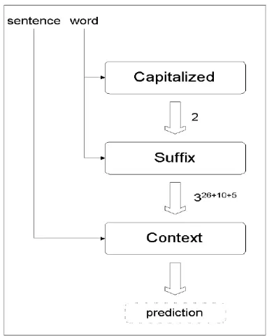
is a single classifier that uses the same information as used by the SM. Fig 1
Figure 1: POS Tagging of Unknown Word using
Contextual and Lexical features in a Sequential Model. The input for capitalized classifier has 2 values and therefore 2 ways to create confusion sets. There are at most &F
k
+! different
in-puts for the suffix classifier (26 character + 10 digits + 5 other symbols), therefore suffix may emit up to &R
k
+R confusion sets.
illustrates the SM that was used in the experiments.
All the classifiers in the sequential model, as well as the single classifier, use the SNoW learn-ing architecture (Roth, 1998) with the Winnow up-date rule. SNoW (Sparse Network of Winnows) is a multi-class classifier that is specifically tai-lored for learning in domains in which the poten-tial number of features taking part in decisions is very large, but in which decisions actually depend on a small number of those features. SNoW works by learning a sparse network of linear functions over a pre-defined or incrementally learned feature space. SNoW has already been used successfully on several tasks in natural language processing (Roth, 1998; Roth and Zelenko, 1998; Golding and Roth, 1999; Punyakanok and Roth, 2001).
Specifically, for each class label SNoW learns a function [K_^ that maps a feature based representation` of the input instance to a number
[image:4.612.329.520.72.312.2]prob-ability of being the class label corresponding to` . At prediction time, given`3a , SNoW outputs
-/
J' ¡SU`nY/G%
`
Sl`iY_: (1)
All functions – in our case, ,' target nodes are used, one for each pos tag – reside over the same feature space, but can be thought of as autonomous functions (networks). That is, a given example is treated autonomously by each target subnetwork; an example labeled is considered as a positive exam-ple for the function learned for and as a negative example for the rest of the functions (target nodes). The network is sparse in that a target node need not be connected to all nodes in the input layer. For ex-ample, it is not connected to input nodes (features) that were never active with it in the same sentence.
Although SNoW is used with,' different targets, the SM utilizes by determining the confusion set dy-namically. That is, in evaluation (prediction), the
maximum in Eq. 1 is taken only over the currently
applicable confusion set. Moreover, in training, a given example is used to train only target networks that are in the currently applicable confusion set. That is, an example that is positive for target , is viewed as positive for this target (if it is in the con-fusion set), and as negative for the other targets in the confusion set. All other targets do not see this example.
The case of POS tagging of known words is han-dled in a similar way. In this case, all possible tags are known. In training, we record, for each word
2
, all pos tags with which it was tagged in the training corpus. During evaluation, whenever word
2
oc-curs, it is tagged with one of these pos tags. That is, in evaluation, the confusion set consists only of those tags observed with the target word in train-ing, and the maximum in Eq. 1 is taken only over these. This is always the case when using (orT
), both in the SM and as a single classifier. In training, though, for the sake of this experiment, we treat (T
) differently depending on whether it is trained for the SM or as a single classifier. When trained as a single classifier (e.g., (Roth and Zelenko, 1998)),
uses each -tagged example as a positive exam-ple for and a negative example for all other tags. On the other hand, the SM classifier is trained on a
-tagged example of word , by using it as a posi-tive example for and a negative example only for the effective confusion set. That is, those pos tags which have been observed as tags of in the train-ing corpus.
4.2 Experimental Results
The data for the experiments was extracted from the Penn Treebank WSJ and Brown corpora. The train-ing corpus consists of WF5'P' words. The test corpus consists of ¢WP' words of which ,RTK are unknown words (that is, they do not occur in the training corpus. (Numbers (the pos “CD”), are not included among the unknown words).
POS Tagging of Unknown Words
+ baseline baseline
¢W¤£ £¤¢ £W¤¢
Table 1: POS tagging of unknown words using
contextual features (accuracy in percent). is
a classifier that uses only contextual features, + baseline is the same classifier with the addition of the baseline feature (“NNP” or “NN”).
Table 1 summarizes the results of the experiments with a single classifier that uses only contextual fea-tures. Notice that adding the baseline POS signifi-cantly improves the results but not much is gained over the baseline. The reason is that the baseline feature is almost perfect (
]5¥ ) in the training data. For that reason, in the next experiments we do not use the baseline at all, since it could hide the phenomenon addressed. (In practice, one might want to use a more sophisticated baseline, as in (Dermatas and Kokkinakis, 1995).)
E
SM(
:_
&
P ) SM(P
&
_T )
¢¤£ ,£ £,W¤¦ ¦'W¤
Table 2: POS tagging of unknown words using
contextual and lexical Features (accuracy in
per-cent). is based only on contextual features,T
is based on contextual and lexical features. SM(
2
_#§ ) denotes that § follows
2
in the sequential model.
Table 2 summarizes the results of the main exper-iment in this part. It exhibits the advantage of using the SM (columns 3,4) over a single classifier that makes use of the same features set (column 2). In both cases, all features are used. In E
, a classifier is trained on input that consists of all these features and chooses a label from among all class labels. In -/.
Sk _
&
_ Y the same features are used as input, but different classifiers are used sequentially – using only part of the feature space and restricting the set of possible outcomes available to the next classifier in the sequence –
2
It is interesting to note that further improvement can be achieved, as shown in the right most column. Given that the last stage in
-/. Sk:_
&
PE
Y is iden-tical to the single classifier T
, this shows the con-tribution of the filtering done in the first two stages using
and
&
. In addition, this result shows that the input spaces of the classifiers need not be dis-joint.
POS Tagging of Known Words
Essentially everyone who is learning a POS tagger for known words makes use of a “sequential model” assumption during evaluation – by restricting the set of candidates, as discussed in Sec 4.1). The fo-cus of this experiment is thus to investigate the ad-vantage of the SM during training. In this case, a single (one-vs-all) classifier trains each tag against
all other tags, while a SM classifier trains it only
against the effective confusion set (Sec 4.1). Table 3 compares the performance of the clas-sifier trained using in a one-vs-all method to the same classifier trained the SM way. The results are only for known words and the results of Brill’s tag-ger (Brill, 1995) are presented for comparison.
one-vs-all SM| ¨R©
2
Brill
£W¤¢'¢
£W¤¢'£
£]
Table 3: POS Tagging of known words using
con-textual features (accuracy in percent). one-vs-all
denotes training where example` serves as positive example to the true tag and as negative example to all the other tags. SM| ¨R©
2
denotes training where example` serves as positive example to the true tag and as a negative example only to a restricted set of tags in based on a previous classifier – here, a sim-ple baseline restriction.
While, in principle, (see Sec 5) the SM should do better (an never worse) than the one-vs-all classifier, we believe that in this case SM does not have any performance advantages since the classifiers work in a very high dimensional feature space which al-lows the one-vs-all classifier to find a separating hy-perplane that separates the positive examples many different kinds of negative examples (even irrelevant ones).
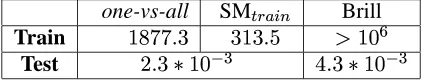
However, the key advantage of the SM in this case is the significant decrease in computation time, both in training and evaluation. Table 4 shows that in the pos tagging task, training using the SM is 6 times faster than with a one-vs-all method and 3000 faster than Brill’s learner. In addition, the evaluation
time of our tagger was about twice faster than that of Brill’s tagger.
one-vs-all SM|¨F©
2
Brill
Train ¢:¦¦¤ Wª, u0
Test WZ1«1
d
T¤=«1
d
Table 4: Processing time for POS tagging of
known words using contextual features (In CPU
seconds). Train: training time over + sentences.
Brill’s learner was interrupted after 12 days of train-ing (default threshold was used). Test: average number of seconds to evaluate a single sentence. All runs were done on the same machine.
5 The Sequential model: Theoretical
Justification
In this section, we discuss some of the theoretical aspects of the SM and explain some of its advan-tages. In particular, we discuss the following issues:
1. Domain Decomposition: When the input fea-ture space can be decomposed, we show that it is advantageous to do it and learn several clas-sifiers, each on a smaller domain.
2. Range Decomposition: Reducing confusion set size is advantageous both in training and testing the classifiers.
(a) Test: Smaller confusion set is shown to yield a smaller expected error.
(b) Training: Under the assumptions that a small confusion set (determined dynam-ically by previous classifiers in the se-quence) is used when a classifier is eval-uated, it is shown that training the classi-fiers this way is advantageous.
3. Expressivity: SM can be viewed as a way to generate an expressive classifier by building on a number of simpler ones. We argue that the SM way of generating an expressive clas-sifier has advantages over other ways of doing it, such as decision tree. (Sec 5.3).
[image:6.612.322.533.110.150.2]5.1 Decomposing the Domain
Decomposing the domain is not an essential part of the SM; it is possible that all the classifiers used ac-tually use the same domain. As we shown below, though, when a decomposition is possible, it is ad-vantageous to use it.
It is shown in Eq. 2-7 that when it is possible to decompose the domain to subsets that are condition-ally independent given the class label, the SM with classifiers defined on these subsets is as accurate as the optimal single classifier. (In fact, this is shown for a pure product of simpler classifiers; the SM uses a selective product.)
In the following we assume that
RsA provide a decomposition of the domain (Sec. 3) and that SU`
F` A Y¬aLSU
F A Y . By condi-tional independence we mean that
CED k®fSU`E2 F` § hY/ § ¯ ° B±2 fSU` ° hKY# where` °
is the input for the² th classifier.
³´!µv¶}³· F¸ X f¹Sg:h`iY/ ³´!µv¶}³· F¸ X f¹Sl5h` R` A Y (2) ³´Rµ ¶}³· F¸ X f¹Sl` R`EAºhKY¼»Rf¹SgY f¹SU` R` A Y (3) ³´Rµ ¶}³· F¸ X f¹Sl` R` A
hKY¼»Rf¹SgY (4)
³´Rµ ¶}³· F¸ X f¹Sl`
hYi»»»lf¹Sl` A hKY¼»RfSlKY (5)
³´Rµ ¶}³· F¸ X f¹Sg:h` Ylf¹Sl` Y fSlKY »»» f¹Sg:h`EA1YUfSU`±A=Y f¹SgY »!f¹SlKY (6) ³´Rµ ¶}³· F¸ X f¹Sg:h`
Yi»»»gf¹Sg:h` A Y6»
fSlKY A d (7) f¹Sl`
R` A Y in Eq. 3 is identical
C
za3 and there-fore can be treated as a constant. Eq. 5 is derived by applying the independence assumption. Eq. 6 is de-rived by using the Bayes rule for each termf¹Sg:h`
2
Y
separately.
We note that although the conditional indepen-dence assumption is a strong one, it is a reasonable assumption in many NLP applications; in particu-lar, when cross modality information is used, this assumption typically holds for decomposition that is done across modalities. For example, in POS tag-ging, lexical information is often conditionally in-dependent of contextual information, given the true
POS. (E.g., assume that word is a gerund; then the context is independent of the “ing” word ending.)
In addition, decomposing the domain has signif-icant advantages from the learning theory point of view (Roth, 1999). Learning over domains of lower dimensionality implies better generalization bounds or, equivalently, more accurate classifiers for a fixed size training set.
5.2 Decomposing the range
The SM attempts to reduce the size of the candidates set. We justify this by considering two cases: (i) Test: we will argue that prediction among a smaller set of classes has advantages over predicting among a large set of classes; (ii) Training: we will argue that it is advantageous to ignore irrelevant examples.
5.2.1 Decomposing the range during Test
The following discussion formalizes the intuition that a smaller confusion set in preferred. Let ¡
½M be the true target function andf¹Sg § h`nY the probability assigned by the final classifier to class
R§¾a given example `¿ap . Assuming that the prediction is done, naturally, by choosing the most likely class label, we see that the expected er-ror when using a confusion set of size² is:
À)ÁÁ J Á ° ÀÃÂ [ÄS ÁÅ % `
!Æ § Æ
°
fSl § h`nYRY=ÇȼSl`iY4^
fSRS ÁÅ % `
!Æ § Æ
°
fSl § h`nYRY=ÇȼSl`iY!Y (8)
Now we have:
Claim 1 LetÉÊ*K R
°
5PÉ˱*K !
°
¨
be two sets of class labels and assume6SU`nYta0É
for example` . Then À$ÁÁ J Á °Ì À)ÁÁ J Á °_Í . Proof. Denote: fTÎ5S PÏPnY6fSRS ÁÅ % ` ©Æ § ÆEÐ
fSl § h`iY!Y=ÇȼSl`iY!Y
Then, À$ÁÁ J ÁKÑ Í ÀÃÂ [ S ÁÅ % `
!Æ § Æ
°
¨
f¹Sg§ h`nYRY=ÇÒ6SU`nY{^
Claim 1 shows that reducing the size of the con-fusion set can only help; this holds under the as-sumption that the true class label is not eliminated from consideration by down stream classifiers, that is, under the one-sided error assumption. Moreover, it is easy to see that the proof of Claim 1 allows us to relax the one sided error assumption and assume instead that the previous classifiers err with a prob-ability which is smaller than:
SR( À$ÁÁ
J
Á
Ñ
Y6»RfTÎ5S{²$Ôr'P²$Ô
Á
P6SU`nYRYj
5.2.2 Decomposing the range during training
We will assume now, as suggested by the previous discussion, that in the evaluation stage the small-est possible set of candidates will be considered by each classifier. Based on this assumption, Claim 2 shows that training this way is advantageous. That is, that utilizing the SM in training yields a better classifier.
Let × be a learning algorithm that is trained to minimize: Ø
Â
¸ÙÛÚ
SlÜ»KݹSl`iY!YUfSU`nYÞ:`¼
where ` is an example, Üraß(_Ôm is the true class, Ý is the hypothesis,
Ú
is a loss function and
f¹Sl`iY is the probability of seeing example ` when `sà
e
(see (Allwein et al., 2000)). (Notice that in this section we are using general loss function
Ú
; we could use, in particular, binary loss function used in Sec 5.2.) We phrase and prove the next claim, w.l.o.g, the case of vs. class labels.
Claim 2 Let00KR
&
!j be the set of class
la-bels, let
-2
be the set of examples for classD
. Assume a sequential model in which class does not
com-pete with class . That is, whenever`áa
the
SM filters out such that the final classifier (
A
) considers only and
&
. Then, the error of the hy-pothesis - produced by algorithm× (for
A
) - when trained on examples in
-&
is no larger than
the error produced by the hypothesis it produces when trained on examples in
-&
- .
Proof. Assume that the algorithm × , when
trained on a sample
-, produces a hypothesis that minimizes the empirical error over
-. Denote `Ûà
e
X
when` is sampled according to a distribution that supports only examples with label in . Let
-be a sample set of size% , according to !â
&
, and Ý the hypothesis produced by × . Then, for all ÝÛÇÒÝ ,
%äã
Â
¸å
Ú
SlÜÝ SU`nYRY
Ì
%pã
Â
¸å
Ú
SlÜݹSl`iY!Y (9)
In the limit, as%æqç
Ø
ÂKèié O{êQ
Ú
SUÜÝ
Sl`iY!YUf¹Sl`iYFÞ:`
Ì
Ø
ÂKèié O{êQ
Ú
SlÜݹSl`iY!YUfSU`nYÞ:`¼
In particular this holds if Ý is a hypothesis pro-duced by× when trained on
-, that is sampled ac-cording to`ëà
e
Râ
&
â .
5.3 Expressivity
The SM is a decision process that is conceptually similar to a decision tree processes (Rasoul and Landgrebe, 1991; Mitchell, 1997), especially if one allows more general classifiers in the decision tree nodes. In this section we show that (i) the SM can express any DT. (ii) the SM is more compact than a decision tree even when the DT makes used of more expressive internal nodes (Murthy et al., 1994).
The next theorem shows that for a fixed set of functions (queries) over the input features, any bi-nary decision tree can be represented as a SM. Ex-tending the proof beyond binary decision trees is straight-forward.
Theorem 3 Letì be a binary decision tree with
internal nodes. Then, there exist a sequential model
-such that
-and ì have the same size, and they
produce the same predictions.
Proof (Sketch): Given a decision tree ì on
nodes we show how to construct a SM that produces equivalent predictions.
1. Generate a confusion set the consists of
classes, each representing an internal node in
ì .
2. For each internal node inÞta3ì , assign a clas-sifier:
2
'îí3È\[]#^
"
d
nï . 3. Order the classifiers K¤
A
4. Define each classifier
2
that was assigned to node Þa ì to have an influence on the outcome iff node Þða ì lies in the path (Ï_'!ÏK !Ï
°
d
) from the root to the predicted class.
5. Show that using steps 1-4, the predicted target ofì and
-are identical.
This completes that proof and shows that the result-ing SM is of equivalent size to the original decision tree.
We note that given a SM, it is also relatively easy (details omitted) to construct a decision tree that produces the same decisions as the final classifier of the SM. However, the simple construction results in a decision tree that is exponentially larger than the original SM. Theorem 4 shows that this difference in expressivity is inherent.
Theorem 4 Let
be the number of classifiers in a sequential model
-and the number of internal nodes a in decision tree ì . Let % be the set
of classes in the output of
-and also the maxi-mum degree of the internal nodes inì . Denote by
ñ
Slì=Yj
ñ
S
-Y the number of functions representable
by ì
-respectively. Then, when%òu)u
, ñ
S
-Y
is exponentially larger thanñ Slì=Y .
Proof (Sketch): The proof follows by counting
the number of functions that can be represented using a decision tree with
internal nodes(Wilf, 1994), and the number of functions that can be rep-resented using a sequential model on
intermedi-ate classifier. Given the exponential gap, it follows that one may need exponentially large decision trees to represent an equivalent predictor to an
size SM.
6 Conclusion
A wide range and a large number of classifica-tion tasks will have to be used in order to perform any high level natural language inference such as speech recognition, machine translation or question answering. Although in each instantiation the real conflict could be only to choose among a small set of candidates, the original set of candidates could be very large; deriving the small set of candidates that are relevant to the task at hand may not be immedi-ate.
This paper addressed this problem by developing a general paradigm for multi-class classification that
sequentially restricts the set of candidate classes to a small set, in a way that is driven by the data ob-served. We have described the method and provided some justifications for its advantages, especially in NLP-like domains. Preliminary experiments also show promise.
Several issues are still missing from this work. In our experimental study the decomposition of the feature space was done manually; it would be nice to develop methods to do this automatically. Bet-ter understanding of methods for thresholding the probability distributions that the classifiers output, as well as principled ways to order them are also among the future directions of this research.
References
L. E. Allwein, R. E. Schapire, and Y. Singer. 2000. Reducing multiclass to binary: a unifying ap-proach for margin classifiers. In Proceedings
of the 17th International Workshop on Machine Learning, pages 9–16.
E. Brill. 1995. Transformation-based error-driven learning and natural language processing: A case study in part of speech tagging. Computational
Linguistics, 21(4):543–565.
E. Charniak. 1993. Statistical Language Learning. MIT Press.
I. Dagan, L. Lee, and F. Pereira. 1999. Similarity-based models of word cooccurrence probabilities.
Machine Learning, 34(1-3):43–69.
E. Dermatas and G. Kokkinakis. 1995. Automatic stochastic tagging of natural language texts.
Computational Linguistics, 21(2):137–164.
T. G. Dietterich and G. Bakiri. 1995. Solving multi-class learning problems via error-correcting out-put codes. Journal of Artificial Intelligence
Re-search, 2:263–286.
Y. Even-Zohar and D. Roth. 2000. A classification approach to word prediction. In NAALP 2000, pages 124–131.
W. A. Gale, K. W. Church, and D. Yarowsky. 1993. A method for disambiguating word senses in a large corpus. Computers and the Humanities, 26:415–439.
A. R. Golding and D. Roth. 1999. A Winnow based approach to context-sensitive spelling correction.
Machine Learning, 34(1-3):107–130. Special
Pro-ceedings of the 3rd workshop on very large cor-pora, ACL-95.
T. Hastie and R. Tibshirani. 1998. Classifica-tion by pairwise coupling. In Michael I. Jordan, Michael J. Kearns, and Sara A. Solla, editors,
Advances in Neural Information Processing Sys-tems, volume 10. The MIT Press.
G. Hinton. 2000. Training products of experts by minimizing contrastive divergence. Technical Report GCNU TR 2000-004, University College London.
T. Kudoh and Y. Matsumoto. 2000. Use of sup-port vector machines for chunk identification. In
CoNLL, pages 142–147, Lisbon, Protugal.
L. Lee and F. Pereira. 1999. Distributional similar-ity models: Clustering vs. nearest neighbors. In
ACL 99, pages 33–40.
L. Lee. 1999. Measure of distributional similarity. In ACL 99, pages 25–32.
V.I. Levenshtein. 1966. Binary codes capable of correcting deletions, insertions and reversals. In
Sov. Phys-Dokl, volume 10, pages 707–710.
S.E. Levinson, A. Ljolje, and L.G. Miller. 1990. Continuous speech recognition from phonetic transcription. In Speech and Natural Language
Workshop, pages 190–199.
L. Mangu and E. Brill. 1997. Automatic rule ac-quisition for spelling correction. In Proc. of the
International Conference on Machine Learning,
pages 734–741.
A. Mikheev. 1997. Automatic rule induction for unknown word guessing. In Computational
Lin-guistic, volume 23(3), pages 405–423.
T. M. Mitchell. 1997. Machine Learning. Mcgraw-Hill.
S. Murthy, S. Kasif, and S. Salzberg. 1994. A sys-tem for induction of oblique decision trees.
Jour-nal of Artificial Intelligence Research, 2:1:1–33.
V. Punyakanok and D. Roth. 2001. The use of clas-sifiers in sequential inference. In NIPS-13; The
2000 Conference on Advances in Neural Infor-mation Processing Systems.
S. S. Rasoul and D. A. Landgrebe. 1991. A sur-vey of decision tree classifier methodology. IEEE
Transactions on Systems, Man, and Cybernetics,
21 (3):660–674.
D. Roth and D. Zelenko. 1998. Part of speech tagging using a network of linear separators. In COLING-ACL 98, The 17th International
Conference on Computational Linguistics, pages
1136–1142.
D. Roth. 1998. Learning to resolve natural lan-guage ambiguities: A unified approach. In Proc.
National Conference on Artificial Intelligence,
pages 806–813.
D. Roth. 1999. Learning in natural language. In
Proc. Int’l Joint Conference on Artificial Intelli-gence, pages 898–904.
L-W. Teow and K-F. Loe. 2000. Handwritten digit recognition with a novel vision model that ex-tracts linearly separable features. In CVPR’00,
The IEEE Conference on Computer Vision and Pattern Recognition, pages 76–81.
H. S. Wilf. 1994. generatingfunctionology. Aca-demic Press Inc., Boston, MA, second edition. D. Yarowsky. 1994. Decision lists for lexical
ambi-guity resolution: application to accent restoration in Spanish and French. In Proc. of the Annual
Meeting of the ACL, pages 88–95.
J. Zavrel, W. Daelemans, and J. Veenstra. 1997. Resolving pp attachment ambiguities with mem-ory based learning. In Computational Natural
Language Learning, Madrid, Spain, July.
J. M. Zelle and R. J. Mooney. 1996. Learning to parse database queries using inductive logic pro-gramming. In Proc. National Conference on