Parsimonious Data Oriented Parsing

Parsimonious Data-Oriented Parsing

Willem Zuidema

Institute for Logic, Language and Computation, University of Amsterdam

Plantage Muidergracht 24 1018 TV, Amsterdam, the Netherlands

[email protected]

Abstract

This paper explores a parsimonious ap-proach to Data-Oriented Parsing. While al-lowing, in principle, all possible subtrees of trees in the treebank to be productive elements, our approach aims at finding a manageable subset of these trees that can accurately describe empirical distributions over phrase-structure trees. The proposed algorithm leads to computationally much more tracktable parsers, as well as linguis-tically more informative grammars. The parser is evaluated on the OVIS and WSJ corpora, and shows improvements on effi-ciency, parse accuracy and testset likelihood.

1 Data-Oriented Parsing

Data-Oriented Parsing (DOP) is a framework for statistical parsing and language modeling originally proposed by Scha (1990). Some of its innovations, although radical at the time, are now widely ac-cepted: the use of fragments from the trees in an annotated corpus as the symbolic grammar (now known as “treebank grammars”, Charniak, 1996) and inclusion of all statistical dependencies between nodes in the trees for disambiguation (the “all-subtrees approach”, Collins & Duffy, 2002).

The best known instantiations of the DOP-framework are due to Bod (1998; 2001; 2003), using the Probabilistic Tree Substitution Grammar (PTSG) formalism. Bod has advocated a maximal-ist approach to DOP, inducing grammars that con-tain all subtrees of all parse trees in the treebank,

and using them to parse unknown sentences where all of these subtrees can potentially contribute to the most probable parse. Although Bod’s empirical re-sults have been excellent, his maximalism poses im-portant computational challenges that, although not necessarily unsolvable, threaten both the scalability to larger treebanks and the cognitive plausibility of the models.

In this paper I explore a different approach to DOP, that I will call “Parsimonious Data-Oriented Parsing” (P-DOP). This approach remains true to Scha’s original program, by allowing, in principle, all possible subtrees of trees in the treebank to be the productive elements. But unlike Bod’s approach, P-DOP aims at finding a succinct subset of such el-ementary trees, chosen such that it can still accu-rately describe observed distributions over phrase-structure trees. I will demonstrate that P-DOP leads to computationally more tracktable parsers, as well as linguistically more informative grammars. More-over, as P-DOP is formulated as an enrichment of the treebank Probabilistic Context-free Grammar (PCFG), it allows for much easier comparison to al-ternative approaches to statistical parsing (Collins, 1997; Charniak, 1997; Johnson, 1998; Klein and Manning, 2003; Petrov et al., 2006).

2 Independence Assumptions in PCFGs Parsing with treebank PCFGs, in its simplest form, involves the following steps: (1) a treebank is cre-ated by extracting phrase-structure trees from an an-notated corpus, and split in a train- and a testset; (2) a PCFG is read off from all productions in the trainset trees, with weights proportional to their

quency in the treebank (the “relative frequency esti-mate”); (3) a standard PCFG parser is used to find for each yield of the test-set trees the most probable parse; (4) these parses are compared to the test-set trees to count matching brackets, labels and trees.

PCFGs incorporate a strong statistical indepen-dence assumption: that the expansion of a nonter-minal node is only dependent on the node’s label. All state-of-the-art wide-coverage parsers relax this assumption in some way, for instance by (i) chang-ing the parser in step (3), such that the application of rules isconditioned on other steps in the deriva-tion process (Collins, 1997; Charniak, 1997), or by (ii) enriching the nonterminal labels in step (1) with context-information (Johnson, 1998; Klein and Manning, 2003), along with suitable backtransforms in step (4). These two approaches often turn out to be equivalent, although for some conditionings it is not trivial to work out the equivalent enrichment and vice versa, especially when combined with smooth-ing. Interesting recent work has focused on the au-tomatic induction of enrichments (Matzuzaki et al., 2005; Prescher, 2005), leading to extremely accurate parsers (Petrov et al., 2006).

DOP relaxes the independence assumption by changing the class of probabilistic grammars in-duced in step (2). In DOP1 (Bod, 1998), a PTSG is induced, which consists, subject to some heuris-tic constraints, of all subtrees1 _{of the treebank} trees with a weight proportional to their frequency. PTSGs allow multiple derivations to yield the same parse; in DOP1 the sum of their probabilities gives the probability of the parse. The relation between DOP and enrichment/conditioning models was clar-ified by Joshua Goodman, who devised an efficient PCFG transform of the DOP1 model (Goodman, 1996). The size of the PCFG resulting from this transform is linear in the number of nonterminals to-kens in the corpus. Goodman’s transform, in com-bination with a range of heuristics, allowed Bod (2003) to run the DOP model on the Penn Treebank WSJ benchmark and obtain some of the best results obtained with a generative model.

The computational challenges for DOP are far from solved, however. The difference with style

1_{A subtreet}0of a parse tree

tis a tree such that every node i0in

t0equals a node

iint, andi0either has no daughters or the

same daughter nodes asi.

(ii) enrichment is that we derive many more rules from every original tree than the number of CFG-productions it contains. This is one reason why the relative frequency estimator for DOP is inconsistent (Johnson, 2002). But worse, perhaps, the size of the grammar remains gigantic2_{, making it difficult for} many in the field to replicate Bod’s results.

In this paper, we develop a parsimonious ap-proach to DOP, that avoids many of the computa-tional problems of the maximalist approach but tries to maintain its excellent empirical performance. Our approach starts, both conceptually and technically, with an analysis of where the PCFG independence assumption breaks down when modeling empirical distributions. In section 2 we derive equations for the expected frequency of arbitrary subtrees under a distribution defined by a given PCFG, and use them to measure how much observed subtree-frequencies deviate from expectation. In section 4 we generalize this analysis to PTSGs. In section 5 we discuss an al-gorithm for estimating PTSGs from a treebank, that is based on minimizing the differences between ex-pected and observed subtree-frequencies. We then proceed with discussing PTSGs induced from var-ious treebanks, and in section 6 the use of these PTSGs for parsing.

3 Deviations from a PCFG distribution PCFGs can be viewed as PTSGs where the elemen-tary trees are restricted to depth 1; we therefore start by repeating the definition of PTSGs (Bod, 1998), and use notation appropriate for PTSGs throughout. An PTSG is a 5-tuplehVn, Vt, S, T, wi, whereVnis

the set of non-terminal symbols;Vt is the set of

ter-minal symbols;S ∈Vnis the start symbol;T is a set

of elementary trees, such that for everyτ ∈ T the

unique root node r(τ) ∈ Vn, the (possibly empty)

set of internal nodes i(τ) ⊂ Vn and the set of leaf

nodesl(τ) ⊂ Vn∪Vt; finally,w : T → [0,1]is a

probability (weight) distribution over the elementary trees, such that for anyτ ∈T,P_τ0_∈R(τ)w(τ0) = 1,

whereR(τ) is the set of elementary trees with the

same root label as τ. It will prove useful to also

define the set of all possible treesθover the defined 2_{Sections 2-21 of WSJ contain1676821productions. Of}

these,106 _{are lexical productions, and36151top-productions,}

alphabets (with the same conditions on root, internal and leaf nodes as forT), and the set of all possible

completeparse trees Θ(with r(t) = S and all leaf

nodesl(t)⊂Vt). Obviously,T ⊂θandΘ⊂θ.

The substitution operation◦is defined if the

left-most nonterminal leaf inτ1 is identical to the root

ofτ2. Performing substitutionτ1◦τ2 yieldst3, ift3

is identical toτ1 with the leftmost nonterminal leaf

replaced by τ2. A derivation is a sequence of

ele-mentary trees, where the first treeτ ∈ T has

root-label S and every next tree combines through

sub-stitution with the result of the subsub-stitutions before it. In this paper, we are only concerned with gram-mars that define proper probability distributions over trees, such that the probability of all derivations sum up to1and no probability mass gets lost in

deriva-tions that never reach a terminal yield. That is, we require (ift(d)is the tree derived by derivationd):

X

d:t(d)∈Θ

P(d) = 1. (1)

For simplicity, but without loss of generality, we as-sume there are no recursions on the start symbol.

In this section, we restrict ourselves to PCFG dis-tributions, and thus to a T with only depth 1 trees.

The probability of a PCFG rule (conditioned on its left-hand side) in the conventional notation,P(A7→ αβ . . . γ|A), now corresponds to the probability of a

depth 1 tree (conditioned on its root nonterminal):

P  

A

α β . . . γ

|A  

Of course, the probability of a (complete) deriva-tion is simply the product of the (condideriva-tional) prob-abilities of the rules in the derivation. It is useful to consider, for a given grammar Ggenerating a

cor-pus of N trees, the expected frequency of visiting

nonterminal stateX:

EF(X) = (

N ifX =S

P

τEF(τ)C(X, l(τ)) otherwise

(2) whereC(X, l(τ))gives the number of occurrences

of nonterminal X among the leaves of elementary

tree τ. Furthermore, the expectedusage frequency

ofτ is given by

EF(τ) = EF(r(τ))P(τ|r(τ))

= EF(r(τ))w(τ) (3)

Substituting eq (3) into (2) yields a system of

|Vn| linear equations, that can be straightforwardly

solved using standard methods.

We are interested in the empirical deviations from the distribution defined by a given grammar (for in-stance, the treebank PCFG), such that we can adjust the grammar to better model the training data (whilst avoiding overfitting). In line with the general DOP approach, we would like to measure this deviation for every possible subtree. Of course, the condi-tional probability of an arbitrary subtree is simply the product of the rule probabilities. The expected frequency of a subtree is the expected frequency of its root state, times the conditional probability:

EF(t) =EF(r(t))P(t|r(t)) (4)

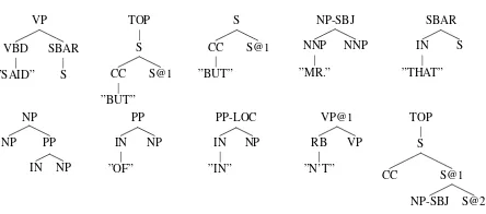
Using these equations, we can measure for each observed subtree in the corpus, the difference be-tween observed frequency and expected frequency. This will give high values for overrepresented and frequent constructions in the corpus, such as sub-trees corresponding torevenues rose CD % to$CD million from$CD million last year,details weren’t disclosed, NP-SUBJ declined to commentand con-tracted and negated auxiliaries such aswon’t,can’t and don’t. The top-10 overrepresented subtrees in the WSJ20-corpus are given in figure 1.

VP VBD ”SAID”

SBAR S

TOP S CC ”BUT”

S@1 S CC ”BUT”

S@1

NP-SBJ NNP ”MR.”

NNP

SBAR IN ”THAT”

S

NP NP PP

IN NP

PP IN ”OF”

NP

PP-LOC IN ”IN”

NP

VP@1 RB ”N’T”

VP TOP

S

CC S@1 NP-SBJ S@2

Figure 1: Top-10 overrepresented subtrees (excluding subtrees with punctuation) in sentences of length≤20, including punc-tuation, in sections 2-21 of the WSJ-corpus (transformed to Chomsky Normal Form, whereby newly created nonterminals are marked with an @). Measured are the deviations from the expected frequencies according to the treebank PCFG (of this selection), as in equation (4) but withEF(r(t))replaced by the empirical frequencyo(r(t)). Observed frequencies are (deviations between brackets): 461 (+408.2), 554 (+363.8), 556 (+361.7), 479 (+348.2), 332 (+314.3), 415 (+313.3), 460 (+305.1), 389 (+283.0), 426 (+277.2), 295 (+266.1).

ones, e.g.revenues rose CD from$CD million from

$ CD million. Underrepresented subtrees found in the WSJ20 corpus, include (VP (VBZ ”IS”) NP)), which occurs only once, even though it is predicted 152.7 times more often (in all other VP’s with “IS”, the NP is labeled NP-PRD); and (PP (IN ”IN”) NP)), which occurs 38 times but is expected 121.0 times more often (IN NP-constructions are usually labeled PP-LOC).

Given such statistics, how do we improve the grammar such that it better models the data? PCFG enrichment models (Klein and Manning, 2003; Schmid, 2006) split (and merge) nonterminals; in automatic enrichment methods (Prescher, 2005; Petrov et al., 2006) these transformations are per-formed so as to maximize data likelihood (under some constraints). The treebank PCFG-distribution thereby changes, such that the deviations from fig-ure 1 mostly disappear. For instance, the overrepre-sentation of “but” as the sentence-initial CC in the second and third subtree of that figure, is dealt with in (Schmid, 2006) by splitting the CC-category into CC/BUT and CC/AND. However, also when a range of such transformations is applied, some subtrees are still greatly overrepresented. Figure 2 gives the top-10 overrepresented subtrees of the same treebank, enriched with Schmid’s enrichment programtmod. In DOP, larger subtrees can be explicitly repre-sented as units. This is the approach we take in this paper, which involves switching from PCFGs to PTSGs. However, we cannot simply add over-represented trees to the treebank PCFG; as is clear from figure 2, many of the overrepresented subtrees are in fact spurious variations of the same construc-tions (e.g. “$ CD million”, “a JJ NN”). To reach our goal of finding the minimal set of subtrees that ac-curately models the empirical distribution over trees, we will thus need to consider a series of PTSGs, find the subtrees that are still overrepresented and adapt the grammar accordingly.

4 Deviations from an PTSG distribution

4.1 Expected Frequencies: An Example

Once we allow T to contain elementary trees of

depth larger than 1, the equations above become

more difficult. The reason is that now multiple derivations may give rise to the same parse tree, and,

NP-SBJ/3S/BASE NNP ”MR.”

NNP@1 QP/$ $ QP/$@1

CD CD@1 ”MILLION”

NP-SBJ/BASE NNP ”MR.”

NNP@1 ] QP/$ $ ”$”

QP/$@1 CD CD@1

”MILLION” QP/$@1

CD CD@1 ”MILLION”

NP/BASE

DT/A NP/BASE@1 JJ NN

VP/FIN

MD VP/FIN@1 RB/NOT VP/INF

NP/BASE

DT/A ”A”

NP/BASE@1 JJ NN TOP

NP-SBJ/3S/BASE NNP ”MR.”

NNP@1 S/FIN/.@1

NP/BASE

NNP NP/BASE@1

NNP@1 NP/BASE@2

Figure 2: Top-10 overrepresented subtrees (excluding subtrees with punctuation) in the WSJ20 corpus, enriched with thetmod

program (Schmid, 2006). Empirical frequencies are as fol-lows (deviations between brackets): 262 (+207.6), 235 (+158.4) 207 (+156.4), 228 (+153.5), 237 (+141.0), 190 (+134.2), 153 (+126.5), 166 (+117.8), 139 (+110.0), 111 (+103.8).

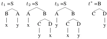
as a corrolary, a specific subtree can emerge in many different ways. Consider an PTSG that consists of all subtrees of the treest1,t2 andt3in figure 3, and

the expected frequency of the subtreet∗.

t₁=S B x

A y

t₂=S A x

B C y

D x

t₃=S A

y B C x

D y

t∗=B

C D y

Figure 3: Three example treebank trees and the focal subtree

It is clear that t∗ might arise in many different ways. For instance, it emerges in the derivation with elementary treesτ1◦τ4◦τ5from figure 4, but also in

derivationsτ2◦τ4andτ3◦τ5. Note that in none of

these derivations elementary treet∗itself was used.

τ₁=S A x

B C D

τ₂= S A

y B C D

y τ₃= S

A x

B C y

D τ₄= C

x τ₅=D

y τ₆=B

C D

Figure 4: Some elementary trees extracted from the trees in fig 3

4.2 Expected Frequency: Usage & Occurrence

Hence, when using PTSGs, we need to distinguish between theexpected usage frequencyof an elemen-tary tree (written asEu(τ)), and theexpected

occur-rence frequency (Eo(t)) of the corresponding

de-rived tree are necessarily “visited” substitution sites. The expected frequency of visiting a nonterminal stateX as substitution site depends on the usage

fre-quencies:

EF(X) = (

N ifX =S

P

τEu(τ)C(X, l(τ)) otherwise

(5) Relating usage frequencies to weights is still sim-ple (compare equation 3):

Eu(τ) =EF(r(τ))w(τ) (6)

And hence: w(τ) =Eu(τ)/P_τ0_:r(τ)=r(τ0₎Eu(τ0).

The expected frequency of a complete tree is not simply a product anymore, but the sum of the differ-ent derivation probabilities (where der(t) gives the

set of derivations oft):

Eo(t) = X

d∈der(t)

Y

τ∈d

w(τ) ift∈Θ (7)

4.3 Expected Frequency of Arbitrary Subtrees

Most complex is the expected occurrence frequency of an arbitrary subtreet. From the example above it

is clear that it is not necessary that the root oftis a

substitution site. Analogous to equation (4), we need the expected frequency of arriving at some stateσin

the derivation process that is still consistent with ex-panding to something that containst, and multiply it

with the probability that this expansion indeed hap-pens:

Eo(t) =X

σ

EF(σ)P(t|σ) (8)

To be able to define the states σ, we redefine the

set of derivationsder(t)of a subtreet, such that the

derivationsder(t∗₎of our example tree from figure 3 are the following: d1 =B ◦τ6◦τ5,d2 = τ6◦τ5,

d3 =B◦t∗andd4 =t∗. Only if a derivation starts

with a single nonterminal is the root node consid-ered a substitution site. The states σ correspond to

the first elements of each of these derivations, i.e.

hB, τ6, B, t∗i.

As was clear from the example in section 4.1, we need to consider all supertrees of the trees in the derivation oftfor calculating the expected

fre-quency of a state and the probability of expanding from that state to form t. It is useful to

distin-guish, as do Bod & Kaplan (Bod, 1998, ch. 10) two

types of supertree-subtree relations, depending on whether nodes must be removed from the root down-ward, or from the leaves (“frontier”) upward. “Root-subtrees” of tare those subtrees headed by any of t’s internal nodes and everything below.

“Frontier-subtrees” are those subtrees headed byt’s root-node,

pruned at any number (≥0) of internal nodes. Using ◦to indicate left-most substitution, we can write:

• t1is aroot-subtreeoft1, andt1is aroot-subtree

oft2, if∃t3, such thatt3◦t1 =t2;

• t1is afrontier-subtreeoft1, andt1is a

frontier-subtreeoft2, if∃t3. . . tn, such thatt1◦t3. . .◦

tn=t2.

• t0 is the _x-frontier-subtree of_t,_t0 _{= f s} x(t), if xis a set of nodes int, such that iftis pruned

at eachi∈xit equalst0.

We use the notationst(t)for the set of subtrees of t,rs(t)for the set of root-subtrees oftandf s(t)for

the set of frontier-subtrees oft. Thus defined, the set

of all subtrees oftis the set of all frontier-subtrees

of all root-subtrees of t: st(t) = {t0_|∃t00_(t00 _∈

rs(t)∧t0 _{∈ f s(t}00₎₎. We further define the sets of root-supertrees, frontier-supertrees, and supertrees as follows: (i) f sdx(t) = {t0|t = f sx(t0)}, (ii) c

f s(t) ={t0_{|t∈f s(t}0_)}(iii)_{st(t) =b {t}0_|t∈st(t0_)}. If there are only terminals in the yield oft, the

ex-pected frequency of a stateσis now simply the sum

of the expected usage frequencies of those elemen-tary trees that haveσat theirfrontier(i.e. thatσis a

root-subtree of):

EF(σ) = X

τ0_:σ∈rs(τ0₎ Eu(τ0

) ifl(t)⊂Vt (9)

If there are nonterminals in the yield oft, as in the

example, we need to also consider elementary trees that have these nonterminals already expanded. To see why, consider again the example of section 4.1 and check that also elementary treeτ3contributes to

the expected frequency of t∗. If we take this into account, and writent(t)for the nonterminal nodes

in the yield oft, the final expression for the expected

frequency of stateσbecomes:

EF(σ) = X

τ∈f sb(σ)

X

τ0_∈rsd

nt₍t₎(τ)

Eu(τ0

Finally, the probability of expanding a state σ

such thattemerges is again simplest ifthas no

non-terminals as leaves. Remember that a stateσwas the

first element of a derivation oft; the probability of

expanding totis simply the product of the weights

of the remaining elementary trees in the derivation (if states are unique for a derivation):

P(t|σ) = Y

τ∈rest(d)

w(τ) ifl(t)⊂Vt (11)

If there are nonterminals among the leaves of t,

however, we need again to sum over possible expan-sions at those nonterminal leaves:

P(t|σ) = Y

τ∈rest(d)

X

τ0_{∈f s}d

x₍t₎(τ)

w τ0 (12)

Substituting equations (9) and (12) into equa-tion (8) gives a general expression for the expected occurrence frequency of an arbitary subtreet:

Eo(t) = X

d∈der_(t)

Y

τ∈

rest(d₎

X

τ0_{∈f s}d

x₍t₎(τ)

w τ0

X

τ∈ b

rs₍first₍d₎₎

X

τ0_{∈f s}d

x(t)(τ)

Eu(τ0

)

. (13)

5 Minimizing deviations: estimation The equations just derived can be used to learn an PTSG from a treebank, using an estimation proce-dure we call “push-n-pull” (pnp). This procedure was described in some detail elsewhere (Zuidema, 2006b); here I only sketch the basic idea. Given an initial setting of the parameters (all depth 1 el-ementary trees at their empirical frequency), the method calculates the expected frequency of all complete and incomplete trees. If a tree t’s

ex-pected frequency Eo(t) is higher than its observed

frequency o(t), the method subtracts the difference

from the tree’s score, and distributes (“pushes”) it over the elementary trees involved in all its deriva-tions (der(t)). If it is lower, it “pulls” the difference

from all its derivations.

The “score” of an elementary tree τ is the

al-gorithm’s estimate of the usage frequency u(τ).

The amounts of score that are pushed or pulled are

capped by the requirement that∀τ u(τ) ≥0;

more-over, the learning rate parameter γ determines the

fraction of the expected-observed difference that is actually pushed or pulled. Finally, the method in-cludes a bias (B) for moving probability mass to

smaller elementary trees, to avoid overfitting (its ef-fects become smaller as more data gets observed).

Because smaller elementary trees will be involved in other derivations as well, the push and pull opera-tions will shift probabilities between different parse trees. Suppose a given complete tree is the only tree with nonzero frequency of all trees that can be built from the same components. This tree will continue to “pull” until it has in fact reached its appropriate frequency. Similarly, if a given tree does have zero observed frequency, it will continue to leak score to other derivations with the same components.

NP/BASE

DT/A NP/BASE@1 JJ NN

NP-SBJ/3S/BASE NNP ”MR.”

NNP1

NP/BASE

DT/THE ”THE”

NP/BASE@1 JJ NN

NP-SBJ/BASE NNP ”MR.”

NNP1

NP/GEN/BASE

NNP NP/GEN/BASE@1 NNP1 POS

”’S”

NP/PP

NP/BASE PP/OF/NP IN/OF

”OF” NP/BASE1

NP/BASE

NNP NP/BASE@1 NNP1 NNP2

NP/BASE JJ NP/BASE@1

JJ1 NNS

NP QP/$ $ QP/$@1

CD CD1 ”MILLION”

VP/FIN

MD VP/FIN@1 ADVP/V

RB/V VP/INF

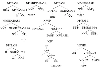
Figure 5: Top-10 elementary trees of depth>1, excluding those with punctuation, from runningpnpon the enriched WSJ20.

No thank you, I want PP to VP-INF, I want PP, I want Prep NP-LOC Prep NP-LOC, Yes please, At CD o’clock. In figure 5 we give the top-10 elemen-tary trees resulting from the WSJ20-corpus.

Figure 6: Log-log curves of (i) subtree frequencies against rank (for106 _{subtrees from WSJ20), (ii)pnp-scores against rank,}

and (iii) the same for the top-10000 depth>1-subtrees.

Figure 6 shows some characteristics of this last grammar. Shown are log-log plots, such as com-monly used to visualise the Zipf-distributions in nat-ural language. The top curve plots log(frequency) against log(rank) for each subtree of the trees in the corpus, which shows the approximate Zipfian behavior. The second curve from above plots the log(score) against log(rank) for these same subtrees. As can be observed, the score-distribution follows the frequency distribution only for the most frequent subtrees (all of depth 1), but then deviates from it downwards. The bottom curve – an almost straight line in this log-log space – gives the log(score) vs log(rank) of subtrees with a depth>1.

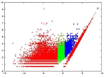
Figure 7: Subtree frequencies againstpnp-scores, including subsets pnp1000 (dark/blue) and pnp10000 (light/green).

Figure 7 further illustrates the difference between the score- and the frequency-distributions, by

plot-ting for each subtree, log-frequency (y-axis) against log-score (x-axis). The subtrees clearly fall into two categories: those where the scores correlate strongly with frequency (the depth 1 subtrees) and the larger subtrees that vary greatly in how strong scores corre-late with frequency. Only larger subtrees that receive relatively high scores should be used in parsing.

Weights are proportional to subtree-frequencies in the DOP1 and related “maximalist” models. The differences between the frequency and score-distributions thus illustrate a very important differ-ence between maximalist and parsimonious DOP. The characteristics of the score distribution allow P-DOP to throw away most of the subtrees without significantly affecting the distribution over complete parse trees that the grammar defines. This is the ap-proach we take for evaluating parsing performance: we take as our baseline the treebank PCFG, and then add the n larger elementary trees with the highest

scores from our induced PTSG.

6 Parsing Results

For our parsing results we use BitPar, a fast and freely available general PCFG parser (Schmid, 2004). In our first experiments we used the OVIS corpus, with semantic tags and punctuation re-moved, and all trees (train- and testset) binarized. As a baseline experiment, we read off the treebank PCFG as decribed in section 2. The recall, precision and complete match results are in table 1, labeled tb-pcfg. For comparison, we also show the results ob-tained with two versions of the DOP model, DOP1 (Bod, 1998) and DOP* (Zollmann and Sima’an, 2005) on the same treebank.

We ran the pnpprogram as described above on the trainset, with parametersB = 1.0,γ = 0.1and d= 4. This run yielded a single PTSG that was used

in 4 parsing runs. For these experiments, we added increasingly many of the depth>1 elementary trees

auto-matically sums (and substracts) and normalizes the frequency information provided with each rule. Bit-Par was then run on the testset sentences, with the option to output the nbest parses withn = 10by

default. These parses were then read in in a post-processing program, which removes address labels, sums probabilities of equivalent parses and outputs the most probable parse for each sentence (this is the same approximation of MPP, albeit with smaller n,

as used in most of Bod’s DOP results). The results of these experiments are also in table 1, labeled pnpN,

whereN is the number of elementary trees added.

model #rules LR LP CM

tb-pcfg 3000 93.45 95.5 85.84

DOP1 1.4×106 (87.55)

DOP* (<50000) (87.7)

pnp100 3000+100 93.63 95.65 86.55 pnp763 3000+763 93.5 95.52 86.75 pnp1517 3000+1517 93.78 95.83 87.36 pnp11411 3000+11411 94.26 96.4 87.77

Table 1: Results on the Dutch OVIS tree bank, with semantic tags and punctuation removed. Reported are evalb scores on a random testset of 1000 sentences (a second testset of 1000 sen-tences is kept for later evaluations). The trainset for both the treebank grammar and thepnpprogram consists of the remain-ing 8049 trees. Coverage in all cases in 989 sentences out of 1000. Results in brackets are from Zollman & Sima’an, 2005, using a different train-test set split.

As these experiments show, adding larger elemen-tary trees from the induced PTSG, in order of their assigned scores, monotonously increases the parse accuracy of the treebank PCFG. Although the final grammar is at least 5 times larger than the origi-nal treebank PCFG, and the parser therefore slower, the grammar is orders of magnitude smaller than the corresponding maximalist DOP models and shows comparable parse accuracy.

For a second set of parsing experiments, we used the WSJ portion of the Penn Tree Bank (Marcus et al., 1993) and Helmut Schmid’s enrichment program tmod(Schmid, 2006). Schmid’s program enriches nonterminal labels in the treebank, using features in-spired by (Klein and Manning, 2003). After enrich-ment, Schmid obtained excellent parsing scores with the treebank PCFG. In table 2, as model tb-pcfg, we give our baseline results. These are slightly lower than Schmid’s, for two reasons: (i) our

implemen-tation ignores the upper/lower case distinction, and (ii) we do not use Schmid’s word class automaton for unknown words (the only smoothing used is the built-in feature of the BitPar parser, which extracts an open-class-tag file from the lexicon file). Because our interest here is in the principles of enrichment we have not attempted to adapt these techniques for our implementation.

As before, we ran thepnpprogram on the train-set, the enriched sections 2-21 of the WSJ. For computational reasons, pnp is only run on trees with a yield of length (including punctuation) ≤ 20. This run, which took several days on a

ma-chine with 1.5Gb RAM, again produced a very large PTSG, from which we extracted the 1000 and 10000 depth>1 elementary trees with the highest scores

for parsing experiments. Parsing and postprocess-ing is performed as before, with the MPP approxi-mated from the bestn = 20 parses. Results from

these experiments are shown in table 2, as models pnp1000 and pnp10000. With a small number of added trees, we see a small drop in the parsing per-formance, which we interpret as evidence that our additions somewhat disturb the nicely tuned prob-ability distribution of the treebank PCFG without providing many advantages, because the most fre-quent constructions have already been addressed in the manual PCFG enrichment. However, with 10000 added subtrees we see an increase in parse accuracy, providing evidence that pnp has learned potential enrichments that go beyond the manual enrichment.

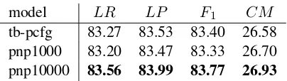
model LR LP F1 CM

tb-pcfg 83.27 83.53 83.40 26.58 pnp1000 83.20 83.47 83.33 26.70 pnp10000 83.56 83.99 83.77 26.93

Table 2: Results on the WSJ section of the Penn Tree Bank, where nonterminals are enriched with features using Helmut Schmid’stmodprogram (Schmid, 2006). Reported are evalb scores (ignoring punctuation) on 1699 sentences≤100, includ-ing punctuation, from section 22. Sections 02-21 were the train set for the treebank PCFG; only trees with a yield (including punctuation) of length≤ 20were used for thepnpprogram. Coverage in all cases is 1691 (excluding failed parses gives F₁= 85.19for the tb-pcfg-baseline, and85.54for pnp10000).

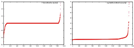
difference. Hence, on the left are sentences where the treebank PCFG scores better, and at the right the sentence where pnp10000 scores best. As is clear from this graph, for most sentences there is no difference, but there are small and about equally sized subsets of sentences for which one or the other model scores better. We have briefly analysed these sentences, but not found a clear pattern. In fig-ure 8(right) we plot in a similar way the difference in log-likelihood that the parsers assign to each sen-tence. Here we see a clear pattern: only very few sentences receive slightly higher likelihood under the PCFG model. For a good portion of the sen-tences, however, the pnp10000 model assigns them somewhat and in some cases much higher likeli-hood. The highest likelihood gains are due to a small number of frequent multiword expressions, such as “New York Stock Exchange Composite Trading”, which P-DOP treats as a unit; all of the other gains in likelihood are also due to the use of depth>1

ele-mentary trees, including some non-contiguous con-structions such asrevenues rose CD % to$CD mil-lion from$CD million.

-60 -40 -20 0 20 40 60

0 200 400 600 800 1000 1200 1400 1600 1800 F-score difference (pnp-tbg)

-10 0 10 20 30 40 50 60 70

0 200 400 600 800 1000 1200 1400 1600 1800 Log-likelihood difference (pnp-tbg)

Figure 8: Per sentence difference in f-score (left) and log-likelihood (right) of the sentences of WSJ section 22. The x-axis gives the sentence-rank when sentences are ordered from small to large on y-axis value.

7 Discussion and Conclusions

We set out to develop a parsimonious approach to Data-Oriented Parsing, where all subtrees can poten-tially become units in a probabilistic grammar but only if the statistics require it. The grammars re-sulting from our algorithm are orders of magnitude smaller than those used in Bod’s maximalist DOP. Although our parsing results are not yet at the level of the best results obtained by Bod, our results in-dicate that we are getting closer and that we already induce linguistically more plausible grammars.

Could P-DOP eventually not only be more effi-cient, but also more accurate than maximalist DOP

models? Bod has argued that the explanation for DOP’s excellent results is that it takes into account all possible dependencies between productions in a tree, and not just those from an a-priori chosen subset (e.g. lexical, head, parent features). Non-head dependencies in non-contiguous natural lan-guage constructions, like more ... than, as inmore freight than cargo, are typically excluded in the en-richment/conditioning approaches discussed in sec-tion 2. Bod wants to include any dependency a pri-ori, and then “let the statistics decide”.

Although the inclusion of all dependencies must somehow explain the performance difference be-tween Bod’s best generative model and manually en-riched PCFG models, this explanation is not entirely satisfactory. Zuidema (2006a) shows that also the estimator (Bod, 2003) uses is biased and inconsis-tent, and will, even in the limit of infinite data, not correctly identify many possible distributions over trees. This is not just a theoretical problem. For instance, in the Penn Tree Bank the construction won’t VPis annotated as(VP (MD wo) (RB n’t) VP). There is a strong dependency between the two mor-phemes: wo doesn’t exist as an independent word, and strongly predictsn’t. However, Bod’s estimator will continue to reserve probability mass for other combinations with the same POS-tags such as wo not, even with an infinite data set only containing will not and wo n’t. Because in parsing the strings are given, this particular example will not harm the parse accuracy results. The example might be di-agnostic for other cases that do, however, and cer-tainly will have impact when DOP is used as lan-guage model. P-DOP, in contrast, does converge to grammars that treatwon’tas a single unit.

The exact relation of P-DOP to other DOP mod-els, including S-DOP (Bod, 2003), Backoff-DOP (Sima’an and Buratto, 2003), DOP* (Zollmann and Sima’an, 2005) and ML-DOP (Bod, 2006; based on Expectation Maximization) and not dissimilar au-tomatic enrichment models such as (Petrov et al., 2006), remains a topic for future work.

References

Rens Bod. 1998. Beyond Grammar: An

experience-based theory of language. CSLI, Stanford, CA.

Rens Bod. 2001. What is the minimal set of fragments

that achieves maximal parse accuracy? In

Proceed-ings ACL-2001.

Rens Bod. 2003. An efficient implementation of a new

DOP model. InProceedings EACL’03.

Rens Bod. 2006. An all-subtrees approach to

unsuper-vised parsing. Proceedings ACL-COLING’06.

Eugene Charniak. 1996. Tree-bank grammars. Techni-cal report, Department of Computer Science, Brown University

Eugene Charniak. 1997. Statistical parsing with a context-free grammar and word statistics. In Proceed-ings of the fourteenth national conference on artificial

intelligence, Menlo Park. AAAI Press/MIT Press.

Michael Collins and Nigel Duffy. 2002. New ranking algorithms for parsing and tagging: Kernels over dis-crete structures, and the voted perceptron. In

Proceed-ings ACL 2002.

Michael Collins. 1997. Three generative, lexicalized models for statistical parsing. In Philip R. Cohen

and Wolfgang Wahlster, editors,Proceedings ACL’97,

pages 16–23.

Joshua Goodman. 1996. Efficient algorithms for parsing

the DOP model. InProceedings EMNLP, pages 143–

152.

Mark Johnson. 1998. PCFG models of

linguis-tic tree representations. Computational Linguistics, 24(4):613–632.

Mark Johnson. 2002. The DOP estimation method is

biased and inconsistent. Computational Linguistics,

28(1):71–76.

Dan Klein and Christopher D. Manning. 2003. Accurate unlexicalized parsing. InProceedings ACL’03. M.P. Marcus, B. Santorini, and M.A. Marcinkiewicz.

1993. Building a large annotated corpus of En-glish: The Penn Treebank.Computational Linguistics, 19(2).

T. Matzuzaki, Y. Miyao, and J. Tsujii. 2005.

Proba-bilistic CFG with latent annotations. InProceedings

ACL’05, pages 75–82.

Slav Petrov, Leon Barrett, Romain Thibaux, and Dan Klein. 2006. Learning accurate, compact, and

in-terpretable tree annotation. In Proceedings

ACL-COLING’06, pages 443–440.

Detlef Prescher. 2005. Inducing head-driven PCFGs with latent heads: Refining a tree-bank grammar for

parsing. InProceedings ECML’05.

Remko Scha. 1990. Taaltheorie en

taaltechnolo-gie; competence en performance. In R. de Kort

and G.L.J. Leerdam, editors,

Computertoepassin-gen in de Neerlandistiek, pages 7–22. LVVN,

Almere, the Netherlands. English translation at

http://iaaa.nl/rs/LeerdamE.html.

Helmut Schmid. 2004. Efficient parsing of highly am-biguous context-free grammars with bit vectors. In

Proceedings COLING 2004.

Helmut Schmid. 2006. Trace prediction and recovery

with unlexicalized PCFGs and slash features. In

Pro-ceedings of COLING-ACL 2006.

Khalil Sima’an. 2002. Computational complexity of

probabilistic disambiguation. Grammars, 5(2):125–

151.

Khalil Sima’an and Luciano Buratto. 2003. Backoff

pa-rameter estimation for the DOP model. InProceedings

of the 14th European Conference on Machine

Learn-ing (ECML’03, Cavtat-Dubrovnik, Croatia, number

2837 in Lecture Notes in Artificial Intelligence, pages 373–384. Springer Verlag, Berlin, Germany.

Gert Veldhuijzen van Zanten, Gosse Bouma, Khalil Sima’an, Gertjan van Noord, and Remko Bonnema. 1999. Evaluation of the NLP components of the OVIS2 spoken dialogue system. In van Eynde,

Schu-urman, and Schelkens, editors, Computational

Lin-guistics in the Netherlands 1998, pages 213–229.

Rodopi, Amsterdam.

Andreas Zollmann and Khalil Sima’an. 2005. A consis-tent and efficient estimator for data-oriented parsing.

Journal of Automata, Languages and Combinatorics,

10(2/3):367–388.

Willem Zuidema. 2006a. Theoretical

evalua-tion of estimaevalua-tion methods for Data-Oriented

Parsing. In Proceedings EACL 2006

(Con-ference Companion), pages 183–186.

Associa-tion for ComputaAssocia-tional Linguistics. Erratum on

http://staff.science.uva.nl/˜jzuidema/research.

Willem Zuidema. 2006b. What are the productive units of natural language grammar? A DOP approach to the automatic identification of constructions. In Proceed-ings of the 10th International Conference on