Abstract—Anomaly detection is automatic identification of
the abnormal behaviors embedded in a large amount of normal data. This paper presents a method based on one class support vector machine (OCSVM) for detecting network anomalies. The telecommunication network performance data are used for the investigation. Firstly, the raw data are preprocessed in order to produce the vector sets required by the OCSVM algorithm. After preprocessing, the vector set of the training data is used to train the OCSVM detector, which is capable of learning the nominal behaviors of the data. The trained detector is then applied on the test data to detect the anomalies. The detected anomalies are finally categorized into major or minor level by comparing with a threshold. In this paper, experiments on three different types of performance data are presented and the results demonstrate the promising performance of the algorithm.
Index Terms—Anomaly detection, one class support vector
machine, telecommunication, time series.
I. INTRODUCTION
Due to the growing number of unauthorized activities in the telecommunication performance data, intelligent management of data and automatic detection of network anomalies are greatly demanded. Network performance data include qualitative data, also known as Key Performance Indicators (KPIs), and quantitative data. These data are used to characterize the network behavior and therefore used for network anomaly detection. In general, an “anomaly” is defined as any occurrence of a value in a data set falling outside of the so-called “normal patterns”, which represent normal and faultless network behavior.
For certain element in the telecommunication network, the data set has its own typical trend, i.e., different types of elements have their typical KPI values. Anything that is suddenly different from the normal or typical value is considered as abnormal and that would indicate an anomaly (or alarm) on the KPI values. Normally, the alarm is generated when there is a sudden drop of the KPI value and in some situations alarm is also generated on a sudden rise of the KPI value. In the current telecommunication system, a pre-defined threshold is normally set for a certain element
Manuscript received January 7, 2008.
R. Zhang is with School of Informatics, University of Bradford, Bradford, United Kingdom, BD7 1DP (phone:+44 (0)1274235462; e-mail: r.zhang2@ bradford.ac.uk).
S. Zhang is with School of Informatics, University of Bradford, Bradford, United Kingdom, BD7 1DP (e-mail: [email protected]).
Y. Lan is with School of Informatics, University of Bradford, Bradford, United Kingdom, BD7 1DP (e-mail: [email protected]).
Prof. J. Jiang is with School of Informatics, University of Bradford, Bradford, United Kingdom, BD7 1DP (e-mail: j.jiang1 @bradford.ac.uk).
and if any drop or increase of the KPI value crosses the threshold, an alarm is generated. As a result of poor setting of the threshold for different indicators or due to very critical situations, the operator screen floods with alarms. If it could become possible to detect abnormal behaviors and provide advance warning of possible anomalies, it may help to suppress the alarms before they propagate across the network. Therefore, artificial intelligence (AI) based detectors are expected to learn the behavior of the indicators and to drastically reduce the volume of alarms presented to the administrator.
Different approaches have been reported by researchers for anomaly detection. Wu et al. [1] proposed a time series analysis approach for network anomaly detection. A wavelet-based signal trend shift detection method was reported in [2]. Keogh et al. [3] introduced a new symbolic representation of time series used for anomalous behavior detection. Other methods include the application of Neural Network [4, 5] and clustering [6]. This paper proposes a method for network anomaly detection based on one class support vector machine (OCSVM). The method consists of two main steps: first is the detector training, the training data set is used to generate the OCSVM detector which is able to learn the nominal profile of the data, and the second step is to detect the anomalies in the performance data with the trained detector.
The rest of this paper is organized as follows: a brief introduction of the OCSVM theory is given in Section II. The data source used in the paper and the proposed anomaly detection algorithm are presented in Section III. Experiments are carried out on three different sets of data and the experimental results are given in Section IV. Conclusions and further work are finally discussed in Section V.
II. METHODOLOGY
In this section, some basic concepts of the OCSVM will be introduced. The support vector machine (SVM) algorithm [7] as it is usually constructed is essentially a two-class algorithm. Scholkopf et al. [8] proposed a method of adapting SVM to one class classification problem. The OCSVM [9, 10, 11] can be considered as a regular two-class SVM where all the training data lies in the first class and the origin is the only member of the second class. The basic idea of the OCSVM is to map the input data into a high dimensional feature space using an appropriate kernel function and constructs a decision function to best separate one class data from the second class data with the maximum margin. In this paper, both the origin and the data that “close enough” to the origin belong to the second class and they are considered as
Network Anomaly Detection Using One Class
Support Vector Machine
the anomalies. Fig.1 gives the geometry interpretation of the OCSVM [12].
Fig. 1. One class SVM classifier.
More specifically, given a training data set without any class information,x Rn i l
i∈ , =1,2,..., , i is the number of data
points in the training set, Rn is the input space and n is the dimension of the input space. Φ(x) is a map function that transforms x from the input space to the feature space F. A hyper-plane or linear decision function f(x) in the feature space F is constructed as
ρ
−
Φ
=
(
)
)
(
x
w
x
f
T(1)
to separate as many as possible of the mapped vectors
} ,..., 2 , 1 ), (
{Φ xi i= l from the origin, w is the norm
perpendicular to the hyper-plane and ρ is the bias of the hyper-plane. In order to solve w and ρ, it needs to solve the following optimization problem,
ρ ξ
ρ ξ
, ,
1 1 2
1 min
w l
i i T
vl w
w
∑
=
− +
(2)
subject to wTΦ(x)≥−ρ −ξi,
ξ
i ≥0,i=1,2,...,lwhere
ξ
i are slack variables that are penalized in the objective function and ν∈(0,1), which is the parameter that controls a trade off between maximizing the distance of the hyper-plane from the origin and the number of data points contained by the hyper-plane, i.e., when v is small, fewer data fall on the same side of the hyper-plane as the origin in the feature space F.In order to solve (2), Largrangian multiplier αi is introduced to each xi and the dual problem of the
optimization problem of (2) can be obtained. Solving the dual problem leads to
∑
=Φ = l
i
i
i x
w 1
) (
α
where
vl
i 1
0 ≤ α ≤ . Accordingly the decision function f(x) becomes a nonlinear function as
∑
=
− = l
i
i iK x x
x f
1
) , ( )
( α ρ (3)
where K(xi,x)=Φ(xi)TΦ(x) [13], which is a kernel function in the input space. There are many admissible choices for kernel function depending on the experience and experiment. Keerthi and Lin [14] reported that Radial Basic Function (RBF), as shown in (4) is the most widely used kernel in SVM, and RBF kernel is adopted in our experiments. For any x, if f(x) is negative, x is detected as an
anomaly, otherwise x is normal. ) 2 / ( 1 2 2 2
)
,
(
x
ix
e
x x σK
=
− − (4)III. EXPERIMENT A. Data Set
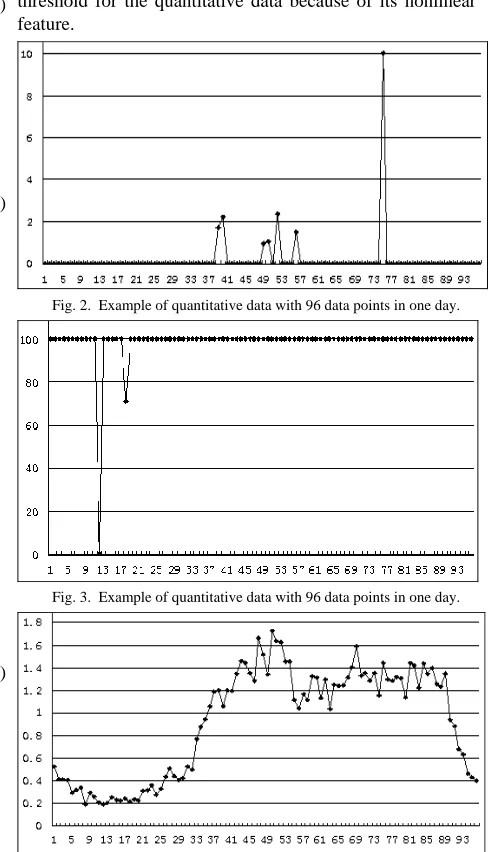
[image:2.612.304.548.304.730.2]As mentioned previously, qualitative data (KPIs) and quantitative data are used for network anomaly detection. KPIs measure the service quality and are recorded in percentage between zero and hundred, such as system interchange success rate. Two KPI examples are shown in Fig. 2 and Fig. 3 with 96 data points for each plot. It can be seen that most of the data points on each plot have the same values, which are zero and one hundred in Fig. 2 and Fig. 3 respectively. Any drop or increase over a certain threshold of such data indicates an anomaly condition. Fig. 4 gives an example of quantitative data, which reflects the change of the network traffic. Most of the quantitative data have the different values and it has its own trend as seen in Fig. 4. It is apparent that it is extremely difficult to set a pre-defined threshold for the quantitative data because of its nonlinear feature.
Fig. 2. Example of quantitative data with 96 data points in one day.
Fig. 3. Example of quantitative data with 96 data points in one day.
In this paper, two KPI data sets as shown in Fig. 2 and Fig. 3 and one quantitative data set as in Fig. 4 are investigated. The recording is made every 15 minutes during 24 hours, and thus 96 data points are obtained throughout one day. Each data set are composed of 31 days data, among which 10 days data with 960 data points are used for training the OCSVM detector and the remaining 21 days data with 2016 data points are used as the test data for the performance evaluation.
B. OCSVM for Anomaly Detection 1) Data Preprocessing
As discussed in Section II, the OCSVM can only be applied to a set of vectors, however in our case the KPI data set is a time series. Therefore, it is necessary to transfer the time series into a set of vectors. Due to the different features of the KPIs and quantitative data, different preprocessing procedures are adopted.
Given a time series of x(t), t =1,2,…..96, x(t) is converted into its feature space Q, where Q∈Rn, and the dimension of Q is set to be n = 2. The time series x(t) is converted into a set of vectors T2 (t) in the feature space Q,
T2 (t) = {X2(t), t=1,2,…,96}.
In OCSCV, as the detection results will be heavily biased to the time series points with either extremely large values, the set of vectors are processed to make sure that most of the values are close to the origin, and thus for the KPI data as in Fig. 2, the corresponding vector set for each data point is
X2(t) = [x(t)/10 x(t)/10], t =1,2,…,96.
Forthe KPI data as in Fig. 3, the vector set is
X2(t) = [(x(t)-100)/10 (x(t)-100)/10], t =1,2,…,96.
For the quantitative data as in Fig. 4, the corresponding vector set is the difference between each pair of the adjacent data points,
X2(t) = [x(t) x(t)], t=1,
X2(t) = [x(t)-x(t-1) x(t)-x(t-1)], t=2,3…,96. C. Model Training and Anomaly Detection
As the RBF kernel is selected for the OCSVM algorithm, two parametersμand σneed to be set before carrying out the training. As described previously, the parameter μ controls a trade off between the fraction of data points in the region and the generalization ability of the decision function. The parameter σ controls the non-linear charasteristics of the decision function. Therefore, both the parameters μ and σ influence the generalization performance of the OCSVM. The choice of such parameters depends on the requirements of the research problem. In our experiments, the two parameters of the algorithm are set as follows:
1) OCSVM parameter μ=0.02; 2) RBF kernel function
) 100 / ( 1 2 2
) ,
(xi x e x x
K = − −
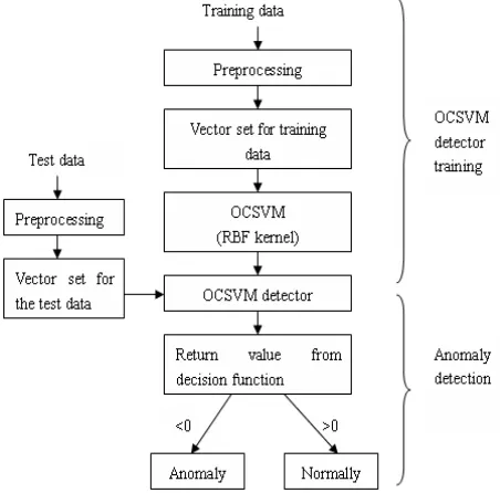
The purpose of OCSVM training is to create the OCSVM detectors that are capable of recognising network KPI profile. Firstly, both the training set and the test set are preprocessed to obtain the vector sets according to their different data types. The training vector set is then used to train the OCSVM detector and the OCSVM detector is then applied on the test vector set. If the return value for the decision function f(x) is negative, an anomaly is detected, otherwise it
[image:3.612.311.537.86.309.2]is normal. This whole procedure of this method is demonstrated in a diagram in Fig. 5.
Fig. 5. Overall procedure of the proposed method.
IV. RESULTS
The experiment results based on both the KPI data and the quantitative data are presented in this section to demonstrate the performance of the algorithm.
A. Results based on the KPI data
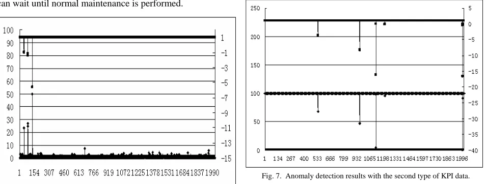
can wait until normal maintenance is performed.
Fig. 6. Anomaly detection results with the first type of KPI data.
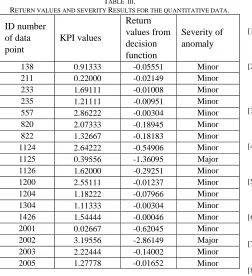
TABLE I.
RETURN VALUES AND SEVERITY RESULTS FOR THE FIRST TYPE OF KPI DATA.
ID number of data point
KPI values
Return value from decision function
Severity of anomaly
43 23.20000 -0.93986 Minor
84 24.82759 -1.13463 Major
85 26.92308 -1.40679 Major
131 50.00000 -5.58027 Major
For the second type of KPI data, the results of anomaly detection are shown in Fig. 7. The upper line on the plot shows the return values of the decision function and the lower line is the plot of the KPI values. 2016 data points recorded in 21 days are included in the plot. As seen in Fig. 7, nine data points of 2016 are detected as the anomalies. The detailed results including the number of the data pointes, the KPI values and the return values of the decision function and the severity of the anomalies are listed in Table II. Five among nine anomalies belong to major type and the remaining four data points are minor anomalies.
B. Results based on the quantitative data
[image:4.612.73.550.50.231.2]Results for anomaly detection of the quantitative data are displayed in Fig. 8. Likewise the KPI data, the upper line in Fig. 8 shows the return values of the decision function and the lower plot shows the original values of the quantitative data. For all the normal values, the return values of the decision function are 1 and for the anomaly data points, the return values are below 0. Again, 2016 data points of 21 days are used for testing and 18 data points are detected as the anomalies. We can see from the plot that the anomalies happen when there is a big drop or increase on the data. These anomalies can also be divided into major or minor type as given in Table III. For exmaple, for data points 1124 and 1125, the quantitative values suddenly dropped from 2.64222 to 0.39556 and a major anomaly is therefore detected.
Fig. 7. Anomaly detection results with the second type of KPI data.
TABLE II.
RETURN VALUES AND SEVERITY RESULTS FOR THE SECOND TYPE OF KPI.
ID number of data point
KPI values
Return value from decision function
Severity of anomaly
538 68.30918 -3.48664 Major
961 47.53623 -8.11106 Major
962 46.66667 -8.31250 Major
1125 98.55072 -0.00805 Minor
1126 4.44444 -16.0747 Major
1214 95.60386 -0.07392 Minor
2000 99.37198 -0.00151 Minor
2001 0.09662 -16.5569 Major
2002 91.11111 -0.30040 Minor
V. CONCLUSION AND FURTHER WORK
Anomaly detection refers to automatic identification of abnormal events existed in a large amount of data and it has been acquiring increasing attention because of its huge potential for application. This paper proposed a network anomaly detection method based on the OCSVM. No a prior knowledge of the normal and abnormal data is required for this method. This algorithm achieves the automated detection of the anomalies and can also support and complement the decisions provided by the current rule-based system.
Fig. 8. Anomaly detection results with the quantitative data.
TABLE III.
RETURN VALUES AND SEVERITY RESULTS FOR THE QUANTITATIVE DATA.
ID number of data point
KPI values
Return values from decision function
Severity of anomaly
138 0.91333 -0.05551 Minor
211 0.22000 -0.02149 Minor
233 1.69111 -0.01008 Minor
235 1.21111 -0.00951 Minor
557 2.86222 -0.00304 Minor
820 2.07333 -0.18945 Minor
822 1.32667 -0.18183 Minor
1124 2.64222 -0.54906 Minor
1125 0.39556 -1.36095 Major
1126 1.62000 -0.29251 Minor
1200 2.55111 -0.01237 Minor
1204 1.18222 -0.07966 Minor
1304 1.11333 -0.00304 Minor
1426 1.54444 -0.00046 Minor
2001 0.02667 -0.62045 Minor
2002 3.19556 -2.86149 Major
2003 2.22444 -0.14002 Minor
2005 1.27778 -0.01652 Minor
This algorithm is more effective than the current rule based systems used by the telecommunication company. In a rule based system, a certain threshold is set for one network element and all the values below the threshold are detected as anomalies. However, the proposed algorithm doesn’t need to have such threshold because the anomaly detector can learn the normal behavior of the KPIs with the training data, and in particularly the anomaly detector can detect new events which have never encountered during the training process. Moreover, after the training cycle is complete, performance results of the algorithms can be also evaluated by the training expert. The training expert has the capability to determine the performance of the detector, i.e., determine whether the anomaly does in fact describe a real problem situation or not. Upon getting the confirmation of real problem or not, the training expert can confirm the detector whether to be accepted or rejected for future testing.
As the use of the OCSVM and the RBF kernel in this work, two parameters μ and σ are needed and further work to find
out the relationship between these parameters and the confidence of the detected anomalies can be considered. Additionally, the ability of the OCSVM to detect anomalies relies on the choice of the kernel and further work can be done on choosing a novel, well-defined kernel which accounts for highly discriminative information and the detection results with different kernels can be also compared. Finally, methods to correlate different KPIs based on the topology to confirm the anomalies can be considered. As the abnormalities, once happen, are not generated in a random order but sequence of connected network elements. Grouping of KPIs based on topology information allows correlation between KPIs from different parts of the network and will result in good correlation. This could further prove the anomalies in the network and reduce the number of the false alarms.
REFERENCES
[1] Q. Wu and Z. Shao, “Network anomaly detection using time series analysis”, Proceedings of the Joint International Conference on Autonomic and Autonomous Systems and International Conference on Networking and Services, vol. 23-28, pp. 42-47, 2005.
[2] C. Shahaibi, X.Tian and W. Zhao, “TSA-tree: wavelet-based approach to improve the efficiency of multi-level surprise and trend queries on time-series data”, Proceedings of 12th International Conference on Scientific and Statistical Database Management, Germany, pp. 1-14, 2002.
[3] E. Keogh, S. Lonardi and W. Chiu, “ Finding surprising patterns in a time series database in linear time and space”, Proceedings of the 8th ACM SIGKDD International Conference on Knowledge Discovery and Data Mining, Canada, pp. 550-556, 2002.
[4] S. Muthuraman and J. Jiang, “Anomaly detection in telecommunication network performance data”, Proceedings of the International Conference on Artificial Intelligence, Las Vegas, Nevada, USA, June, 2007.
[5] S.-J. Han and S.-B. Cho, “Evolutionary neural networks for anomaly detection based on the behavior of a program”, IEEE Transactions on
Systems, Man, and Cybernetics, Part B: Cybernetics, vol. 36, no. 3, 2006.
[6] S. Salvador, P. Chan and J. Brodie, “Learning states and rules for detection anomalies in time series”, Applied Intelligence, vol. 23, no. 3, pp. 241-255, 2005.
[7] C. Burges, “A tutorial on support vector machines for pattern recognition,” Data Mining and Knowledge Discovery, vol. 2, no. 2, pp.121-167, 1998.
[8] B. Schölkopf, J. C. Platt, J. Shawe-Taylor, A.J. Smola and R.C. Williamson, “Estimating the support of a high-dimensional distribution”, Neural Computation, vol. 3, no. 7, pp. 1443-1472, 2001. [9] J. Ma and S. Perkins, “Time-series novelty detection using one-class support vector machines”, Proceedings of the International Joint Conference on Neural Networks, pp. 1741-1745, July, 2003. [10] K. Li, H. Huang, S. Tian and W. Xu, “Improving one-class SVM for
anomaly detection”, Proceedings of the Second International Conference on Machine Learning and Cybernetics, Xi’an, pp. 3077-3081, 2003.
[11] Katherine A Heller, Krysta M Svore, Angelos D. Keromytis, and Salvatore J. Stolfo. “One Class Support Vector Machines for Detecting Anomalous Window Registry Accesses”, Proceedings of the 3rd IEEE Conference Data Mining Workshop on Data Mining for Computer Security,Florida, 2003.
[12] L.M. Manevitz and M. Yousef, “One-Class SVMs for document classification”, Journal of Machine Learning Research, vol. 2, pp. 139-154, 2001.
[13] V.N. Vapnik, “An overview of statistical learning theory”, IEEE Trans.
On Neural Networks, vol. 10, issue 5, pp. 988-999, 1999.
[image:5.612.65.317.244.520.2]