Effects of Nonresponse on the Mean Squared Error of Estimates
from a Longitudinal Study
William D. Kalsbeek, Carolyn B. Morris, Benjamin J. Vaughn , The University of North Carolina at Chapel Hill William D. Kalsbeek, UNC-CH, 730 Airport Road, CB#2400, Chapel Hill, NC 27599-2400
Summary and Background
Research in this study focuses on two related aspects of unit nonresponse (nonresponse by sampled members of study populations) in the rounds of the National Longitudinal Study of Adolescent Health (Add Health) (Chantala and Tabor, 1999): (i) round-specific nonresponse bias and its component contributions, and (ii) the statistical utility of alternative approaches to adjusting sample weights for nonresponse. This work is part of four research studies funded by CDC-NCHS, at the UNC Center for Health Statistics Research.
Nonrespondents in surveys can be classified according to the reason for nonresponse (Lessler and Kalsbeek, 1992): 1) Not Solicited (NS):Sample members are not solicited as perhaps their address is unknown, or they are out of the country; 2) Solicited but Unable (SUA): Sample members are contacted but decline to participate based on inability. Reasons include physical or language limitations; 3) Solicited but Unwilling (SUW): Sample members are contacted but refuse to participate for reasons such as lack of time or, apathy; and 4) Other Nonrespondents (OTH): Sample nonrespondents give a reason that does not fit in any of the previous categories. Examples are lost schedules and partial respondents
Response outcome information and data to obtain 13 different measures of health risk from Add Health are used to accomplish two main tasks in this study. First, we estimate the round-specific nonresponse bias and its component contributions corresponding to the four nonresponse categories described. The sign (negative or positive) of these components and the offsetting effects of some components on the overall bias is of particular interest. Second, we compare the statistical effects of alternate sample adjustments for nonresponse on the bias and variance of study estimates. It is important to note here that we are examining the effects of nonresponse in IH1 and IH2 separately, and not the cumulative effects of nonresponse through these rounds.
The Add Health Study Design
The Add Health study (also known as the National Longitudinal Study Adolescent Health) was designed to identify predictors of adolescent risk behavior and quantify their prevalence. The three rounds to the study began with a self-administered in-school survey (IS1, n=90,118). Two in-person in-home interviews followed: IH1 (n=20,745) and IH2 (n=14,738). The initial sample consisted of 80 high schools and 52 "feeder schools" that
sent students to the selected high schools. Systematic list sampling with probabilities proportional to size (PPS) was used to select the 80 high schools. The measure of size was based on their enrollment as listed on the QED, a database thought to be the most comprehensive available list of schools in the United States (Tourangeau, 1999). For each high school, a middle school was selected as the school that “fed” the most students into its entering class. A number of the high schools also had grades 7-8 and so did not require selection of a feeder school.
All students at the selected schools were asked to take part in IS1. Approximately 200 students from each selected school were asked to complete IH1 and nearly all respondents to IH1 were approached for IH2. The implicit stratification (sampling from a sorted list) resulted in a sample that was nearly representative of all schools in the US. The PPS sampling achieved an almost self-weighting core sample for the in-home portions. Oversampled ethnic groups, twins, siblings, disabled youths, and adopted youths augmented this core sample. Only the core sample was considered in this analysis.
Data collection for IS1 started in September 1994 and ended in April 1995. From April to December 1995, IH1 interviews were conducted. From April to August 1996, respondents to IH1 were approached for IH2. The overall response rate was 78.9% for IH1 and 88.2% for IH2 (20,745 and 14,738 completed interviews, respectively).
The outcome parameters selected for estimation are rates of risk for a number of student health factors. These included the percentage of students who: in the last 12 months, smoked (Smoked), drank alcohol (Drank), were drunk (Drunk), were in a physical fight (Fought), skipped school without an excuse (Skipped), lied to their parents (Lied), and, in the past week, were inactive (Inactive), had poor appetite (No Appetite), felt depressed or blue (Depressed), felt too tired to do things (Tired), did not feel a part of their school (Isolated), felt unhappy at school (Unhappy), and felt unsafe at school (Unsafe). These outcome variables were chosen because they are important public health indicators of risk and were comparably measured in IH1 and IH2.
Method
Bias Profile: To examine the bias and its components arising out of two rounds of Add Health, we used the Hansen-Hurwitz model for quantifying nonresponse bias. This model is a function of the nonresponse rate and the difference between respondents and nonrespondents, as
seen below. Our model presumes that one wishes to estimate the proportion (P) of all members in a population who possess some trait (e.g., at risk to an adverse health outcome), and that
r nr
100λ =100( 1−λ ) percent of the population would be respondents if sampled. If
r P and
nr
P respectively denote the proportion of those in the respondent and nonrespondent subgroups who possess the trait, and Pˆr is an unbiased estimator of
r
P based on respondent data alone but making no effort (for now) to adjust for nonresponse in estimating P, then since
r r ˆ
E( P ) P= and
r r r nr
P=λP ( 1+ −λ )P , the bias due to
the overall nonresponse in the sample can be written as,
o r
ˆ
B ≡Bias( P )=E( P ) Pˆr − =
λ
nr( P P )r− nr . (1) Beyond this expression for the total bias due to nonresponse, Groves (1989) noted that one can view total bias of ˆPr as the sum of components due to various categories of (i.e., reasons for ) nonresponse; i.e., thatC C
( c ) ( c )
o c nr r nr
c 1 c 1
B B
λ
( P P )= =
=
å å
= − (2)where ( c ) ( c )
c nr r nr
B =λ ( P−P ) and
λ
nr( c ) andP
nr( c ) are, respectively, the proportion of the population and the proportion of members with the trait in the c-th nonrespondent category.For any nonrespondent domain, d, (i.e., over all nonrespondents or each of the C nonrespondent categories) one can estimate
d
B as ( d ) ( d )
d nr r nr
ˆ
ˆ ˆ ˆ
B =λ ( P−P ),
where
' ( d ) nr ,d nr '
n ˆ
n
λ = , 'r
r ' r y ˆP
n
= , ( d ) 'nr ,d nr ' ' nr ,d y ˆ P
n
= are weighted
estimates of ( c ) nr
λ
, ( c ) nrP
, andr
P, respectively, and each term with a prime (‘) denotes a Horvitz-Thompson (1952) estimator of a population total; i.e., an estimator of the form n
i i i
w z
å
where iw is the (unadjusted) sample weight and
z
iis the measurement whose population total is being estimated by summing over the sample of size n. Each estimated bias is thus a nonlinear function of five estimated totals. Following the computational strategy suggested by Woodruff (1971), a Taylor Series linearized variance estimate for eachd
ˆB .will be of the form,
h h
2
m m
2
* *
h h h
H
1 1
d
h 1 h
m q q
ˆ v a r ( B )
m 1
α α
α= α=
=
ì ì ü ü
ï −í ý ï
ï î þ ï
= í ý
−
ï ï
ï ï
î þ
å
å
å
(3)where
m
h is the number of sample PSUs in the h-th primary stratum and *h
q
α is the weighted sum (among all respondents in the α-th sample PSU in the h-th stratum) of the Taylor linearized variate corresponding to the five totals defining Bd. A comparable approach was followed in developing the point estimate and its variance for the difference,d B1d B2d
δ = − , between the domain bias for IH1 (
1d
B ) and the bias for the same domain in IH2 ( 2 d B ). The estimate of δd in this case is a function of ten estimated totals and thus requires a different linearized variate for the variance formula.
Comparison of IH2 Nonresponse Adjustments: Estimation in most randomly chosen samples requires that one weight subjects with the inverse of their inclusion probability (Horvitz and Thompson, 1952). These weights are often calculated by the following steps. 1) The raw, or pre-adjustment weight is the inverse of the selection probability, which depends on how the sample was selected. 2) This weight is then multiplied by a factor, called a nonresponse adjustment, to account for the subjects' estimated probability of response, or “response propensity.” 3) These nonresponse-adjusted weights may be calibrated to known population subgroup totals by multiplying them by a post-stratification adjustment. Given our focus on calculating the nonresponse adjustment, we exclude the post-stratification adjustment from further consideration. We will use post-adjustment weight to refer to the product of the pre-adjustment weight and the nonresponse adjustment. We compare variations of two approaches to estimating a respondent’s response propensity in adjusting for IH2 nonresponse: (i) the weighting class adjustment (WCA) estimates the probability using subgroup response rates from the study, and (ii) response propensity modeling (RPM) adjustment uses a fitted logistic model with the response outcome as the dependent variable. The nonresponse adjustment is then obtained as the inverse of the model-derived estimate of the response propensity.
The WCA corrects for nonresponse by dividing the sample into subgroups, or weighting classes, and adjusting the pre-adjustment weight by the inverse of its subgroup response rate. This rate serves as the estimated response propensity for each respondent in the subgroup. Kalton (1983) demonstrated that the bias of the WCA estimator will go to 0 when adjustment cells are chosen such that they are internally homogenous; i.e.,
g ,r g ,nr
outcomes for respondents and nonrespondents. These groupings are often defined by the sample clusters or strata as they are easily accessible and all response rates are known (Lessler and Kalsbeek 1992). This method may overestimate the variance (Kalton 1983), which can be compensated for by either post-stratification or a weight trimming processes (Kalton 1983, Potter 1988).
The RPM adjustment process estimates response probabilities by fitting a logistic model for the response outcome; i.e., an indicator of response status. A criticism of the WCA is that it may not fully utilize the data that are available to the researcher, as it fails to take into account covariates of the outcome variables as well as variables tied more directly to the response mechanism (Sarndal, 1986). Sarndal found that inclusion of such covariates in forming a regression model of the probability of response could reduce the bias of associated estimates.
Many variables may be used as predictors in such a model. Unfortunately, such methods can produce extreme values for the weights, requiring further trimming. The model developed by Deville and Sarndal (1992) imposes bounds on the adjustment factor using a logit based model; for a unit k, the nonresponse adjustment factor is
) Ax ( ) -(1 + 1) -(u ) Ax ( ) -u(1 + 1) -(u = ) ( a k k k λ λ λ ′ ′ exp exp l l
l where xk is the
vector of predictor variables,
l
,
u
are bounds on) (
ak λ ,l<1<u, and A=(u-l)/[(u-1)(1-l)]. Parameters
λ, are estimated using åsxk dk ak(λ)-Tx=0, where Tx is a control data vector and
d
k is the existing weight. This model takes the logit model and adds restrictions, however it does not allow one to choose the lower bound1 ≥
l for nonresponse adjustment, which would be desirable. (Folsom and Singh, 2001).
The generalized exponential model developed by Research Triangle Institute (RTI) (Folsom and Singh, 2001) does this by using the model
) x A ( ) -c ( + ) c -u ( ) x A ( ) -c ( u + ) c -u ( = ) ( a k k k k k k k k k k k k k k k λ λ λ ′ ′ exp exp l l
l as the
adjustment factor, with the parameters λ estimated as before, but using an iterative process. Also, lk,ck,uk can
be chosen separately for each group of observations. As with WCA, these weights add variability to the estimates and can increase the sample variance even while reducing the bias. An advantage of this process is that the weights, since already restricted, do not require subsequent calibration. Also, the restrictions can be used to produce weights appropriate for nonresponse adjustment.
The software used to generate all RPM weight adjustments was developed at RTI (Folsom and Singh 2001). They provided a SAS macro, GEM5.sas, which features nonresponse adjustment as well as post-stratification and extreme value censoring. In our study, only the nonresponse portion was used.
The user-specified parameters for the RTI macro included a list of predictors for which to adjust, the dataset, a unique subject identifier, an indicator for response status, and the existing weights and bounds to put on the returned adjustments. A dataset with subject identifiers and their calculated adjustment based on their responses to the predictors was returned.
The comparative analysis of alternative weighting adjustments was conducted by first generating a number of weighting class (WCAx) and propensity (RPMx) weights using different variables to either form the classes or predict the response outcome, and then multiplying them times the pre-adjustment weight to yield the post-adjustment weight used for estimation. Second, bias, variance and mean squared error (mse) for the health risk estimates were calculated using each of these weights.
Generating alternative adjustments for IH2
nonresponse: Each IH1 respondent was categorized by its
IH2 response status. Further calculations used only IH1 data. A nearest-neighbor bootstrap multiple imputation macro was used for missing values of predictor and weighting cell variables (Quade 2001).
The first adjustment, “WCA1,” was the NORC weighting class nonresponse adjustment, utilizing weighting classes formed by the respondents’ school and gender (Tourangeau, 1999). This was calculated by dividing the sample into 264 weighting cells (132 schools by 2 genders), and giving a nonresponse adjustment factor to each. For the th
h weighting class the adjustment was
computed as, weighted totalh h
weighted resp h
n
n
ϕ
− −=
or weighted RR 1 λ .The second adjustment, “RPM1,” was generated using RTI’s propensity modeling macro, with school and sex as predictors so as to be comparable to WCA1. The weights were calculated by adding the necessary parameters to the macro, which then returned the dataset of the calculated adjustment factors (Chen, 2001).
To produce the adjustment, “RPM2,” we identified several demographic variables, then ran a forward-selection logistic model in SAS v8.01 using these demographics as predictors and IH2 response as outcome (SAS Users Guide, 1999). Variables significant at
α
=0.05 were placed as predictors into RTI’s GEM modeling macro (Chen, 2001; Odom, 2001). For comparison, “WCA2” was created using the significant predictors found in creating RPM2 to split the subjects into weighting classes.determine significant predictors to place into the GEM macro. Although the health variables may be unavailable to researchers in cross-sectional studies, they allowed us to examine the usefulness of data collected in earlier waves to adjust for nonresponse. The final adjustment alternative, “None,” was simply the IH2 pre-adjustment weight with no adjustment for IH2 nonresponse.
Calculating components of the mse: The full set of
IH1 data with the final IH1 pre-adjustment weight was used to calculate 13 health-risk measures. Each IH1 respondent was labeled with his IH2 response status. Nonresponse bias corresponding the each of the six alternative weights was estimated as, Bˆk*=Pˆr ,k−Pˆnr ,None,
the difference between the estimated outcome using the k-th adjustment weight applied to respondent data (Pˆr ,k) and
the outcome using the pre-adjustment weight applied to IH2 respondent and nonrespondent data (Pˆnr ,None). The
magnitude of the bias for each adjustment was then ranked for each outcome variable and averaged among the health risk measures. Proc Surveymeans (SAS Users Guide, 1999) was used to calculate the standard errors of the 13 health risk estimates for each of the nonresponse weights. Last, estimated mse for estimates obtained from each adjusted weight were calculated as 2 2
mse bias= +se and compared as a percent difference to the mse resulting from using IH2 respondent data with no nonresponse
adjustment (msenone); k None
None
mse mse
100
mse
ì − ü
∆= í ý
î þ
. For each
health-risk measure, the
∆
measures were ranked. An average rank was computed for each adjustment.Findings and Discussion
Bias Profile: Estimates of bias for IH1 and IH2
nonresponse in each of 13 measures of health risk prevalence are presented in Table 1. One notes from Table 1 that the magnitude of both total bias and its components for these health indices rarely exceeds 1% in
either IH1 or IH2, which is small relative to the sizes of the prevalence rates which varied mostly from 20% to 80%. Indeed, all but two of the 26 relative total biases, each computed as the estimated total bias divided by the full-sample estimated rate, were less than 2%. Over a quarter of all estimates (8 of 26 total bias and 25 of 104 bias components) were nonetheless found to be statistically significant from zero.
In both IH1 and IH2, the direction of these estimated biases often differed by nonresponse reason. All 26 SUW (refusal) bias estimates were positive, and all but four NS (not solicited) biases were negative (none statistically significant). Directions were mixed for the other categories, with 16 SUA (unable) and 13 OTH bias estimates being positive. These patterns suggest that health risk for those not locatable in Add Health is somewhat higher than for respondents. Alternatively, refusals are at lower risk than respondents, presumably failing to see the need to report their lower risk behavior. Finally, based on the number of statistically significant results, component biases in order of importance were SUW and NS (each 10), SUA (4), and OTH (1).
Contributions of the components to total bias reveal that the greatest magnitude in total biases is seen (“Lied”
and “No Appetite”) when all components are the same sign. Contrastingly, the sum of positive and negative components offsets the total bias. Most intriguing are the three instances (“Unsafe” for IH1 and “Fought” and
“Unhappy” for IH2) where total bias is not significant
and two component biases are significant in the opposite directions. In these instances the relatively strong opposite effects are keeping the total bias in check, and it suggests that altering this balanced state by inducing new nonresponse preventive strategies (e.g., extensive tracking to reduce NS bias) might have the unintended effect of increasing the magnitude of the total bias due to nonresponse, thus making sample estimates more biased than they were.
Table 1: Estimates of Nonresponse Bias (in Percentage Points) for IH1 and IH2 Percent Estimates of Health Risk
IH1 IH2
Variable TOTAL NS SUA SUW OTH Variable TOTAL NS SUA SUW OTH Inactive -0.15 -0.11 -0.04 0.00 0.01 Inactive -0.02 -0.07 -0.02 0.05 0.01
Smoked 0.58 -0.09 0.24 0.37 0.05 Smoked -0.39 -0.30 -0.21 0.17 -0.04
Drank 0.98 -0.05 0.41 0.61 0.02 Drank 0.09 -0.09 -0.06 0.23 0.01
Drunk 0.08 -0.20 0.11 0.17 0.01 Drunk -0.07 -0.04 -0.14 0.14 -0.03
Fought 0.41 -0.04 0.04 0.64 -0.23 Fought -0.34 -0.34 -0.18 0.23 -0.05
Skipped 0.13 -0.14 0.02 0.27 -0.02 Skipped -0.79 -0.57 -0.26 0.08 -0.04
Lied 1.20 0.14 0.37 0.41 0.27 Lied 0.66 0.14 0.16 0.35 0.01
No Appetite 0.82 -0.12 0.34 0.38 0.22 No Appetite 0.31 -0.09 0.16 0.28 -0.03
Depressed 1.23 0.11 0.05 0.80 0.27 Depressed 0.05 -0.16 0.06 0.15 -0.01
Tired 0.52 -0.01 0.15 0.38 0.01 Tired 0.39 0.04 0.07 0.34 -0.06
Isolated -0.18 -0.34 0.09 0.14 -0.08 Isolated -0.31 -0.34 -0.08 0.19 -0.07
Unhappy 0.03 -0.29 0.10 0.15 0.07 Unhappy -0.32 -0.30 -0.19 0.18 0.00
Unsafe 0.10 -0.33 -0.04 0.52 -0.05 Unsafe -0.15 -0.27 0.05 0.10 -0.03
Bolded items indicate significant difference from zero.
NS: Not Solicited
SUW: Solicited But Unwilling
SUA: Solicited But Unable
Table 1 also suggests that biases from IH1 and IH2 are somewhat different. The magnitude of IH1 total biases were generally greater than IH2 biases. Bias components in the two rounds appear to be less different. One possible explanation is that the process circumstances surrounding these two rounds were dissimilar. Nonresponse in IH1 occurred in the context of a first attempt to collect data from a largely unsuspecting sample. Here, the potential respondent knew relatively little about the study and what the interviewer was requesting, suggesting that apprehension and study credibility may have been key considerations by potential respondents, whereas in IH2 a second request for help through study participation was made, thus making respondent burden a major consideration to the response decision maker.
Comparison of IH2 Nonresponse Adjustments:
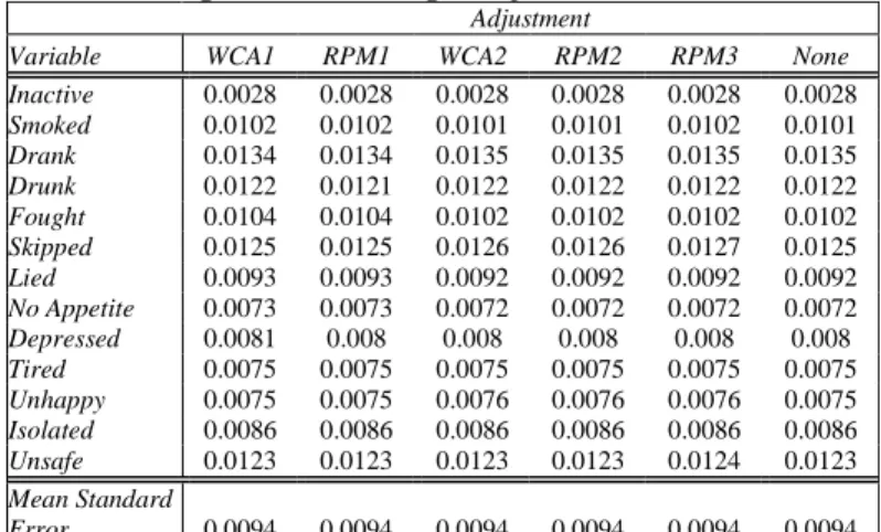
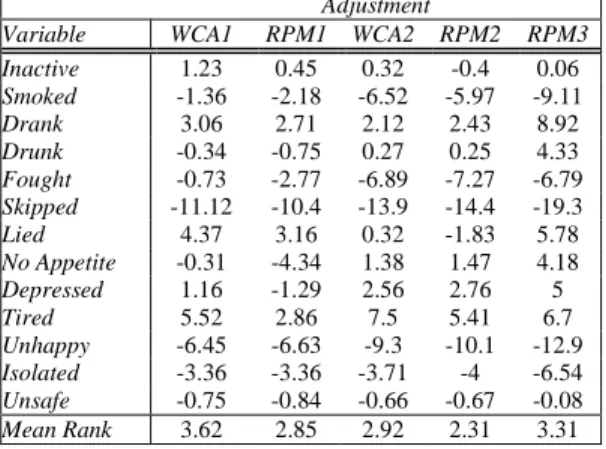
Comparison of (remaining) total bias and of the variance implications of adjustment options applied to IH2 respondents is presented in Tables 2-5. The measures of total bias presented in Table 2 confirm from Table 1 the variable but relatively modest magnitude of bias due to round-specific attrition in the Add Health sample. Observing the ranks of the magnitude (absolute value) of biases for each approach (Table 3) reveals the relative bias-reduction capability of each adjustment option, although individual biases and bias differences among approaches are usually small. A rank of “1” indicates the smallest remaining bias magnitude and “6,” the largest. Comparison of mean ranks revealed that there was no clear winner among the approaches but that the two RPM approaches with the demographic predictors (RPM1 and RPM2) performed best in reducing bias and that, as expected, making no adjustment was statistically the least beneficial. Both WCA approaches were moderate in their level of performance. Most surprising was the somewhat unpredictable utility of the RPM3 approach. For all but three risk measures it was either the best or the worst performer among approaches. Table 4 indicates limited differences in the impact on the variance of estimates of health risk, with the average of estimated standard errors identical to four decimal places. With negligible differences in the effect of adjustment on the variance component of the mse, the performance of these methods relative to the no-adjustment approach are shown in Table 5. As expected, the percent relative differences reported here are mostly negative (indicating reduction in the mse by adjusting for nonresponse), ranging from 0% to nearly -20% (for “Skipped”). An explanation for the positive relative differences is not apparent.
Table 2 Estimated Bias for IH2 Estimates Using Alternative Weight Adjustments
Adjustment
Variable WCA1 RPM1 WCA2 RPM2 RPM3 None Inactive 0.0002 0.0001 0.0001 0.0001 0.0002 -0.0003
Smoked -0.0030 -0.0030 -0.0022 -0.0023 -0.0003 -0.0035
Drank 0.0029 0.0028 0.0025 0.0026 0.0043 0.0015
Drunk 0.0003 0.0003 0.0006 0.0006 0.0023 -0.0006
Fought -0.0019 -0.0014 -0.0008 -0.0008 0.0006 -0.0029
Skipped -0.0057 -0.0058 -0.0050 -0.0049 -0.0034 -0.0076
Lied 0.0078 0.0078 0.0076 0.0074 0.0081 0.0075
No Appetite 0.0035 0.0033 0.0038 0.0038 0.0041 0.0037
Depressed 0.0010 0.0007 0.0016 0.0016 0.0020 0.0008
Tired 0.0045 0.0044 0.0047 0.0045 0.0047 0.0041
Unhappy -0.0029 -0.0029 -0.0024 -0.0023 -0.0016 -0.0036
Isolated -0.0021 -0.0020 -0.0021 -0.0019 -0.0012 -0.0027
Unsafe 0.0000 0.0002 -0.0007 -0.0006 0.0001 -0.0011
Table 3 Ranks of Estimated Biases for IH2 Estimates Using Alternative Weight Adjustments
Adjustment
Variable WCA1 RPM1 WCA2 RPM2 RPM3 None
Inactive 5 3 1 2 4 6
Smoked 5 4 2 3 1 6
Drank 5 4 2 3 6 1
Drunk 2 1 3 4 6 5
Fought 5 4 3 2 1 6
Skipped 4 5 3 2 1 6
Lied 5 4 3 1 6 2
No Appetite 2 1 4 5 6 3
Depressed 3 1 5 4 6 2
Tired 4 2 6 3 5 1
Unhappy 4 5 3 2 1 6
Isolated 5 3 4 2 1 6
Unsafe 1 3 5 4 2 6
Mean Rank 3.85 3.08 3.38 2.85 3.54 4.31
Table 4 Estimated Standard Errors for IH2 Estimates Using Alternative Weight Adjustments
Adjustment
Variable WCA1 RPM1 WCA2 RPM2 RPM3 None Inactive 0.0028 0.0028 0.0028 0.0028 0.0028 0.0028
Smoked 0.0102 0.0102 0.0101 0.0101 0.0102 0.0101
Drank 0.0134 0.0134 0.0135 0.0135 0.0135 0.0135
Drunk 0.0122 0.0121 0.0122 0.0122 0.0122 0.0122
Fought 0.0104 0.0104 0.0102 0.0102 0.0102 0.0102
Skipped 0.0125 0.0125 0.0126 0.0126 0.0127 0.0125
Lied 0.0093 0.0093 0.0092 0.0092 0.0092 0.0092
No Appetite 0.0073 0.0073 0.0072 0.0072 0.0072 0.0072
Depressed 0.0081 0.008 0.008 0.008 0.008 0.008
Tired 0.0075 0.0075 0.0075 0.0075 0.0075 0.0075
Unhappy 0.0075 0.0075 0.0076 0.0076 0.0076 0.0075
Isolated 0.0086 0.0086 0.0086 0.0086 0.0086 0.0086
Unsafe 0.0123 0.0123 0.0123 0.0123 0.0124 0.0123
Mean Standard
Table 5 Estimated Percent Relative Difference in Mean Squared Errors for IH2 Estimates Using Alternative Weight Adjustments *
Adjustment
Variable WCA1 RPM1 WCA2 RPM2 RPM3 Inactive 1.23 0.45 0.32 -0.4 0.06
Smoked -1.36 -2.18 -6.52 -5.97 -9.11
Drank 3.06 2.71 2.12 2.43 8.92
Drunk -0.34 -0.75 0.27 0.25 4.33
Fought -0.73 -2.77 -6.89 -7.27 -6.79
Skipped -11.12 -10.4 -13.9 -14.4 -19.3
Lied 4.37 3.16 0.32 -1.83 5.78
No Appetite -0.31 -4.34 1.38 1.47 4.18
Depressed 1.16 -1.29 2.56 2.76 5
Tired 5.52 2.86 7.5 5.41 6.7
Unhappy -6.45 -6.63 -9.3 -10.1 -12.9
Isolated -3.36 -3.36 -3.71 -4 -6.54
Unsafe -0.75 -0.84 -0.66 -0.67 -0.08
Mean Rank 3.62 2.85 2.92 2.31 3.31
*Relative to the mse of estimates using a pre-adjustment weight
Continuing Work
Since nonresponse carries over from one round to the next, future profiling of bias will examine the cumulative effects of attrition through IH1 and IH2. This assessment is expected to yield biases of larger magnitude as attrition across two rounds approaches 30%. Because of the unusual dynamics with component biases, we will next explore the feasibility of using multinomial logistic models to predict response propensities and adjust weights. Finally, we will explore revising our estimates of variance under the WCA and RPM approaches to handle differential implications of these adjustments on the TSL variance estimates.
REFERENCES
Chantala, K. & Tabor, J. (1999). National Longitudinal Study of Adolescent Health: Strategies to Perform a
Design-Based Analysis Using the Add Health Data.
Chapel Hill, NC: Carolina Population Center, UNC-Chapel Hill
Chen, P.; Penne, M.A., & Singh, A.C. (2001).
“Experience with the Generalized Exponential Model for Weight Calibration for the National Household Survey on Drug Abuse.” Calibration Estimation and Calibration-Adjusted Variance Estimation (A
Methodology R&D Initiative). RTP, NC: Research
Triangle Institute
Deville, J.-C., & Sarndal, C.E. (1992). “Calibration Estimation in Survey Sampling.” Journal of the
American Statistical Association, 87, 376-382.
Folsom, R.E., Jr. & Singh, A.C. (2001). “A Generalized Exponential Model of Sampling Weight Calibration for Extreme Values, Nonresponse and
Poststratification.” Calibration Estimation and Calibration-Adjusted Variance Estimation (A
Methodology R&D Initiative). RTP, NC: Research
Triangle Institute
Groves, R. M. (1989). Survey Errors and Survey Costs, New York: John Wiley & Sons, Inc.
Horvitz, Daniel G. & Thompson, D.J. (1952). “A Generalization of Sampling without Replacement from a Finite Universe.” Journal of the American Statistical
Association, 47, 663-665.
Kalton, Graham. (1983). Compensating for Missing
Survey Research Data. Research Report Series. Ann
Arbor, MI: Institute for Social Research, University of Michigan.
Kish, Leslie. (1965). Survey Sampling. New York: John Wiley & Sons.
Kish, Leslie & Anderson, Dallas W. (1978). “Multivariate and Multipurpose Stratification.”
Journal of the American Statistical Association, 73,
24-34.
Lessler, J.T., & Kalsbeek, W.D. (1992). Nonsampling
Error in Surveys. New York: John Wiley & Sons.
Odom, D. (2001). Personal communication.
Potter, Frank. (1988). “Survey of Procedures to Control Extreme Sampling Weights” ASA Proceedings of the
Section on Survey Research, Alexandria, VA:
American Statistical Association
Quade, D. (2001). Personal communication. Sarndal, C.E. (1986). “A Regression Approach to
Estimation in the Presence of Nonresponse.” Survey
Methodology, 12, 207-215.
SAS Institute, Inc. (1999). SAS/STAT Users Guide,
Version 8. Cary, North Carolina
SAS Institute, Inc. (1999). SAS/STAT Procedures Guide,
Version 8. Cary, North Carolina
Singh, A.C. & Folsom, R.E., Jr. (2001). “Bias Corrected Estimating Function Approach for Variance
Estimation Adjusted for Poststratification.”
Calibration Estimation and Calibration-Adjusted
Variance Estimation (A Methodology R&D Initiative).
RTP, NC: Research Triangle Institute Tourangeau, R. & Shin, H. (1999). National
Longitudinal Study of Adolescent Health: Grand
Sample Weight. Chapel Hill, NC: Carolina Population
Center, UNC-Chapel Hill
Vaish, A.K.; Gordek, H. & Singh, A.C. (2001).
“Variance Estimation Adjusted for Weight Calibration Via the Generalized Exponential Model with
Application to the National Household Survey on Drug Abuse.” Calibration Estimation and Calibration-Adjusted Variance Estimation (A Methodology R&D
Initiative). RTP, NC: Research Triangle Institute
Woodruff, R.S. (1971). “A Simple Method for Approximating the Variance of a Complicated Estimate,” Journal of the American Statistical