ISSN Online: 2161-4725 ISSN Print: 2161-4717
DOI: 10.4236/ijaa.2019.93022 Sep. 19, 2019 302 International Journal of Astronomy and Astrophysics
Models for Velocity Decrease in HH34
Lorenzo Zaninetti
Physics Department, via P.Giuria 1, Turin, Italy
Abstract
The conservation of the energy flux in turbulent jets that propagate in the terstellar medium (ISM) allows us to deduce the law of motion when an in-verse power law decrease of density is considered. The back-reaction that is caused by the radiative losses for the trajectory is evaluated. The velocity de-pendence of the jet with time/space is applied to the jet of HH34, for which the astronomical data of velocity versus time/space are available. The intro-duction of precession and constant velocity for the central star allows us to build a curved trajectory for the superjet connected with HH34. The bow shock that is visible in the superjet is explained in the framework of the theory of the image in the case of an optically thin layer.
Keywords
Herbig-Haro Objects, Bok Globules, Bipolar Outflows
1. Introduction
The equation of motion plays a relevant role in our understanding of the physics of the Herbig-Haro objects (HH) after [1][2]. A common example is to evaluate the velocity of the jet in HH34 as 300 km/s, see [3], without paying attention to its spatial or temporal evolution. A precise evaluation of the evolution of the jet’s velocity with time in HH34 has been done, for example, by [4]. It is, therefore, possible to speak of proper motions of young stellar outflows, see [5][6][7][8].
The first set of theoretical efforts exclude the magnetic field: [9] have modeled the slowing down of the HH 34 superjet as a result of the jet’s interaction with the surrounding environment, [10] have shown that a velocity profile in the jet beam is required to explain the observed acceleration in the position-velocity diagram of the HH jet, [11] found some constraints on the physical and chemical parameters of the clump ahead of HHs and [12] reviewed some important How to cite this paper: Zaninetti, L. (2019)
Models for Velocity Decrease in HH34. International Journal of Astronomy and Astrophysics, 9, 302-320.
https://doi.org/10.4236/ijaa.2019.93022
Received: July 24, 2019 Accepted: September 16, 2019 Published: September 19, 2019
Copyright © 2019 by author(s) and Scientific Research Publishing Inc. This work is licensed under the Creative Commons Attribution International License (CC BY 4.0).
DOI: 10.4236/ijaa.2019.93022 303 International Journal of Astronomy and Astrophysics
understanding of outflows from young stars.
The second set of theoretical efforts include the magnetic field: [13] analysed the HH 1-2 region in the L1641 molecular cloud and found a straight magnetic field of about 130 micro-Gauss; [14] analysed HH 211 and found field lines of the magnetic field with different orientations; [15] analysed HH 111 and found evidence for magnetic braking.
These theoretical efforts to understand HH objects leave a series of questions unanswered or partially answered, as follows:
Is it possible to find a law of motion for turbulent jets in the presence of a medium with a density that decreases as a power law?
Is it possible to introduce the back reaction into the equation of motion for turbulent jets to model the radiative losses?
Can we model the bending of the super-jet connected with HH34?
Can we explain the bow shock visible in HH34 with the theory of the image?
To answer these questions, this paper reviews in Section 2 the velocity observations of HH34 at a 9 yr time interval, Section 3 analyses two simple models as given by the Stoke’s and Newton’s laws of resistance, Section 4 applies the conservation of the energy flux in a turbulent jet to find an equation of motion, Section 5 models the extended region of HH34, the so called “superjet”, and Section 6 reports some analytical and numerical algorithms that allow us to build the image of HH34.
2. Preliminaries
The velocity evolution of the HH34 jet has recently been analysed in [SII] 2, (672 nm), frames and Table 1 in [4] reports the Cartesian coordinates, the velocities, and the dynamical time for 18 knots in 9 years of observations. To start with time, t, equal to zero, we fitted the velocity versus distance with the following power law
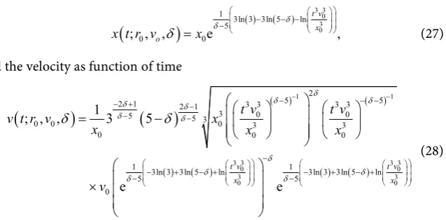
(
; ,0 0)
0(
0)
,v x x v = ×v x x α (1)
where v and x are the velocity and the length of the jet, v0 is the velocity at 0
x x= and
α
with its relative error is a parameter to be found with a fittingprocedure. The integration of this equation gives the time as a function of the position, x, as given by the fit
(
)
1
0 0
0 , 1
x x x
t
v
α α
α
− + −
= −
− (2)
where x0 is the position at t=0. The fitted trajectory, distance versus time, is
(
)
ln( ) (0 ln 10 0 0) 0 0; , e ,
x tv tv x
x t x v α α α
− − + +
−
= (3)
and the fitted velocity as function of time is
(
)
ln( )0 ln( (1 1)0 0)0 0 0 0
1
; , e .
x t v x
v t x v v
x
α
α α
α
− − − +
−
=
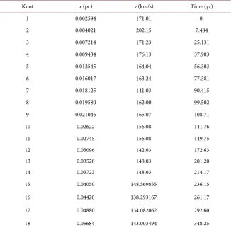
DOI: 10.4236/ijaa.2019.93022 304 International Journal of Astronomy and Astrophysics Table 1. Numerical values for the physical parameters of HH34.
Knot x (pc) v (km/s) Time (yr)
1 0.002594 171.01 0.
2 0.004021 202.15 7.484
3 0.007214 171.23 25.131
4 0.009434 176.13 37.903
5 0.012545 164.04 56.303
6 0.016017 163.24 77.381
7 0.018125 141.03 90.415
8 0.019580 162.00 99.502
9 0.021046 165.07 108.71
10 0.02622 156.08 141.76
11 0.02745 156.08 149.75
12 0.03096 142.03 172.63
13 0.03528 148.03 201.20
14 0.03723 148.03 214.17
15 0.04050 148.569855 236.15
16 0.04420 138.293167 261.17
17 0.04880 134.082062 292.60
18 0.05684 143.003494 348.25
The adopted physical units are pc for length and year for time, and the useful conversion for the velocity is 1 pc year 979682.5397 km s= .
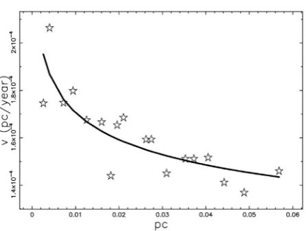
The fit of Equation (1) when x is expressed in pc gives
( )
0.000107 0.0998 0.01618pc yr,v x = x− ± (5)
from which we can conclude that the velocity decreases with increasing distance, see Figure 1.
The time is derived from Equation (2) and Table 1 reports the basic parameters of HH34. This time is more continuous in respect to the dynamical time reported in column 6 of Table 1 in [4].
3. Two Simple Models
When a jet moves through the interstellar medium (ISM), a retarding drag force
drag
F , is applied. If v is the instantaneous velocity, then the simplest model assumes
,
n drag
F ∝v (6)
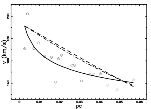
DOI: 10.4236/ijaa.2019.93022 305 International Journal of Astronomy and Astrophysics Figure 1. Observational points of velocity in pc/yr versus distance in pc (empty circles) and best fit as given by Equation (1) (full line).
3.1. Stoke’s Behaviour
The equation of motion is given by( )
( )
d
. d
v t
Bv t
t = − (7)
The velocity as function of time is
0e ,Bt
v v= − (8)
where v0 is the initial velocity. The distance at time t is
( )
0 00
e Bt .
v v
x s t x
B B
−
= = − + (9)
The time as function of distance is obtained by the inversion of this equation
0 0 0
1 ln xB Bx v .
t
B v
− −
= − −
(10) The velocity as a function of space is
(
; , ,0 0)
0 0.v x x v B = −xB Bx v+ + (11)
The numerical value of B is
0 1 0 1
,
v v B
x x
− = −
− (12) where v1 is the velocity at point x1; the data of Table 1 gives B = 0.0009549
(Figure 2).
3.2. Newton’s Behaviour
The equation of motion is( )
( )
2d
. d
v t
Av t
t = − (13)
The velocity as function of time is
( )
00
, 1
v v v t
Atv
= =
DOI: 10.4236/ijaa.2019.93022 306 International Journal of Astronomy and Astrophysics Figure 2. Observational points of velocity in pc/yr versus distance in pc (empty circles), best fit as given by Equation (1) (full line), Stokes behaviour as given by Equation (11) (dashed line) and Newton behaviour as given by Equation (17) (dot-dash-dot-dash).
where v0 is the initial velocity. The distance at time t is
( )
(
0)
0
ln 1
.
Atv
x s t x
A
+
= = + (15)
The time as function of distance is obtained by the inversion of the above equation
0
0
exA Ax 1.
t
Av
− −
= (16)
The velocity as function of the distance is
(
)
0 00 0
; , , .
exA Ax
v
v x x v A = − (17)
The numerical value of A is
0 0 1 1
1 ln v ,
A
x x v
= −
− (18)
where v1 is the velocity at point x1; the data of Table 1 gives A = 5.68381834.
4. Energy Flux Conservation
The conservation of the energy flux in a turbulent jet requires a perpendicular section to the motion along the Cartesian x-axis, A
( )
2A r = πr (19)
where r is the radius of the jet. Section A at position x0 is
( )
0 0tan 2 2A x = πx
α
DOI: 10.4236/ijaa.2019.93022 307 International Journal of Astronomy and Astrophysics
( )
tan 2.2
A x = πx
α
(21) The conservation of energy flux states that
( )
3( )
( ) ( ) ( )
3[
0 0 0
1 1
2ρ x v A x =2ρ x v x A x B (22)
where v x
( )
is the velocity at position x and v x0( )
0 is the velocity at position 0x , see Formula A28 in [16]. More details can be found in [17][18]. The density is assumed to decrease as a power law
0 0 xx
δ
ρ ρ
= (23) where ρ0 is the density at x x= 0 and δ a positive parameter. The differential
equation that models the energy flux is
( )
3 2 3 20
0 0
1 d 1 0.
2 d 2
x x t x v x
x t
δ
− =
(24)
The velocity as a function of the position, x,
( )
2 2 0
3 0 0
0
.
x
x xv
x v x
x x
x δ
δ
=
[image:6.595.202.545.76.402.2] [image:6.595.240.513.478.676.2](25)
Figure 3 reports the velocity as a function of the distance and the observed points.
We now have four models for the velocity as a function of time and Table 2 reports the merit function
χ
2, which is evaluated asFigure 3. Observational points of velocity in pc/yr versus distance in pc (empty stars). The theoretical fit is given by Equation (25) (full line) with parameters x0=0.00259 pc,
0 191.27 km s
DOI: 10.4236/ijaa.2019.93022 308 International Journal of Astronomy and Astrophysics Table 2. The values of the χ2 for four models of velocity of HH34.
Model χ2
Power law fit (no physics) 1479
Stoke’s behaviour 3813
Newton’s behaviour 3317
Turbulent jet 2373
2 2
, , 1
N
i theo i obs
i y y
χ
=
=
∑
− (26)where yi obs, represents the observed value at position i and yi theo, the theo-
retical value at position i. A careful analysis of Table 2 allows us to conclude that the turbulent jet performs better in respect to the Stokes’s and Newton’s behavior.
The trajectory, i.e. the distance as function of the time,
(
)
( ) ( )3 3 0 3 0
1 3ln 3 3ln 5 ln 5
0 0
; , , e ,
t v x o
x t r v δ x δ δ
− − −
−
= (27)
and the velocity as function of time
(
)
(
)
( ) ( )( ) ( ) ( ) ( )
1 1
3 3 3 3
0 0
3 3
0 0
2
5 5
2 1 2 1 3 3 3 3
3 0 0
5 5 3
0 0 0 3 3
0 0 0
1 3ln 3 3ln 5 ln 1 3ln 3 3ln 5 ln
5 5
0
1
; , , 3 5
e e
t v t v
x x
t v t v
v t r v x
x x x
v δ δ δ δ δ δ δ δ δ δ δ δ δ δ − − − − − − + − − − − − + − + − + − + − − = − × (28)
Figure 4 reports the trajectory as a function of time and of the observed points.
The rate of mass flow at the point x, m x
( )
, is(
; ,)
( )
tan 22
m x v alpha =
ρ
v x πx α
(29)
and the astrophysical version is
(
)
(
)
(
)
0 0,km s
2 8 4 3 2 3 2 3 2 3
0 0,km s
; , , ,
7.9252910 tan 2 yr
m x x v M
nx δ x δv M
α α − − + = (30)
where
α
is the opening angle in rad, x and x0 are expressed in pc, n is the number density of protons at x x= 0 expressed in particles cm-3, M is the solar mass and v0,km s is the initial velocity at point x0 expressed in km/s. This [image:7.595.221.540.330.487.2]DOI: 10.4236/ijaa.2019.93022 309 International Journal of Astronomy and Astrophysics Figure 4. Observational points of distance in pc versus time in years (empty stars). The theoretical curve is given by Equation (27) (full line) with the same parameters as in Figure 3.
The Back Reaction
Let us suppose that the radiative losses are proportional to the flux of energy
( ) ( ) ( )
31 ,
2ρ x v x A x
− (31)
where is a constant that is thought to be 1. By inserting in the above equation the considered area, A x
( )
, and the power law density here adopted the radiative losses are2 3 2
0 0
1 tan .
2 2
x v x
x δ
α
ρ
− π
(32)
By inserting in this equation the velocity to first order as given by Equation (25), the radiative losses, Q x x v
(
; , , ,0 0δ
)
, are(
)
3 2(
(
)
)
20 0 1 0 0 0
; , , , tan 2 ,
2
Q x x v δ = − ρ v xπ α x (33)
The sum of the radiative losses between x0 and x is given by the following
integral, L,
(
)
(
)
(
)
0
0 0 0 0
2 3 2
0 0 0 0
; , , , ; , , , d
1 tan .
2 2
x x
L x x v Q x x v delta x
v x x x
δ
α ρ
=
= − π −
∫
(34)
The conservation of the flux of energy in the presence of the back-reaction due to the radiative losses is
3 2 3 3 0 3 2 3 2
0 0 0 0 0 0 0 0
1 1
2 2
x
v x x v x v x v x
x δ ρ ρ − + =
(35)
The real solution of the cubic equation for the velocity to the second order,
(
; , ,0 0)
cv x x v
δ
, is(
)
3(
)
2 2 4 2 20 0 0 0 0 0
; , , 1 .
c
DOI: 10.4236/ijaa.2019.93022 310 International Journal of Astronomy and Astrophysics
Figure 5 reports the effect of introducing the losses on the velocity as function of the distance for a given value of , i.e. the velocity decreases more quickly.
The presence of the back-reaction allows us to evaluate the jet’s length, which can be derived from the minimum in the corrected velocity to second order as a function of x,
(
; , ,0 0)
0, cv x x v
x
δ ∂
=
∂ (37) which is
(
)
(
)
(
)
3 2 3 5 3 3
0 0 0 0
2 3 0
2 2
0. 3 1
v x x x x x x
x x
δ δ
δ
δ
δ
− + − +− − − + − +
=
+ −
(38)
The solution for x of the above minimum allows us to derive the jet’s length,
j
x ,
(
)
0 2 0 2.
1
j x x
x =δ − δ + −δ −
(39)
[image:9.595.270.478.545.694.2]Figure 6 reports an example of the jet’s length as a function of the parameter δ .
Figure 5. Velocity to the second order as function of the distance, see Equation (36), when =0 (full line) and =0.1 (dashed line), other parameters as in Figure 3.
DOI: 10.4236/ijaa.2019.93022 311 International Journal of Astronomy and Astrophysics
5. The Extended Region
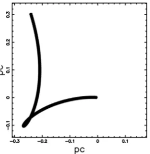
To deal with the complex shape of the continuation of HH34 (e.g. see the new region HH173 discovered by [19]), we should include the precession of the source and motion of the host star, following a scheme outlined in [20]. The various coordinate systems are x=
(
x y z, ,)
, x( )1 =(
x( )1,y z( )1, ( )1)
, ,( )3 =
(
x( )3,y( )3,z( )3)
x . The vector representing the motion of the jet is represented by the following 1 3× matrix:
( )
0 , 0 x t G = (40)where the jet motion L(t) is considered along x axis.
The jet axis, x, is inclined at an angle Ψprec relative to an axis x( )1 , and
therefore the 3 3× matrix, which represents a rotation through z axis, is given by:
(
)
(
)
(
)
(
)
cos sin 0
sin cos 0 .
0 0 1
prec prec
prec prec
F
Ψ − Ψ
= Ψ Ψ
(41)
The jet is undergoing precession around the x( )1 axis and
prec
Ω is the angular velocity of precession expressed in radians per unit time. The transformation from the coordinates x( )1 fixed in the frame of the precessing jet to the nonprecessing
coordinate x( )2 is represented by the 3 3× matrix
(
)
(
)
(
)
(
)
1 0 0
0 cos sin .
0 sin cos
prec prec
prec prec
P t t
t t
= Ω − Ω
Ω Ω
(42)
The last translation represents the change of the framework from (x( )2 ),
which is co-moving with the host star, to a system (x( )3 ), in comparison to
which the host star is in a uniform motion. The relative motion of the origin of the coordinate system
(
x( )3,y( )3 ,z( )3)
is defined by the Cartesian componentsof the star velocity v v vx, ,y z, and the required 1 3× matrix transformation representing this translation is
.
x
y
z
v t B v t v t = (43)
On assuming, for the sake of simplicity, that vx=0 and vz =0, the transla-
tion matrix becomes
0 . 0y B v t
= (44)
DOI: 10.4236/ijaa.2019.93022 312 International Journal of Astronomy and Astrophysics
composing the four matrices already described;
(
)
(
)
( )
(
) (
)
( )
(
) (
)
( )
cos
cos sin .
sin sin
prec
y prec prec
prec prec
x t
A B P F G v t t x t
t x t
Ψ
= + ⋅ ⋅ = + Ω Ψ
Ω Ψ
(45)
The three components of the previous 1 3× matrix A represent the jet’s motion along the Cartesian coordinates as given by an observer who sees the star moving in a uniform motion. The point of view of the observer can be modeled by introducing the matrix E, which represents the three Eulerian angles
, ,
[image:11.595.297.453.273.430.2]Θ Φ Ψ, see [21]. A typical trajectory is reported in Figure 7 and a particularised point of view of the same trajectory is reported in Figure 8 in which a loop is visible.
Figure 7. Continuous trajectory of the superjet connected with HH34: the three Eulerian angles characterising the point of view are Φ =0, Θ =0 and Ψ =0. The precession
is characterised by the angle Ψprec=10 and by the angular velocity 0.00496551674 year
prec
Ω = . The star has velocity 31.107 km s y
v = , the considered time is 29,000 yr and the other parameters are as in Figure 3.
Figure 8. Continuous trajectory of the superjet connected with HH34: the three Eulerian angles characterising the point of view are Φ =100, Θ =77 and Ψ =135. The other
[image:11.595.300.453.523.680.2]DOI: 10.4236/ijaa.2019.93022 313 International Journal of Astronomy and Astrophysics
6. Image Theory
This section summarises the continuum observations of HH34, reviews the transfer equation with particular attention to the case of an optically thin layer, analyses a simple analytical model for theoretical intensity, reports the numerical algorithm that allows us to build a complex image and introduces the theoretical concept of emission from the knots.
6.1. Observations
The system of the jet and counter jet of HH34 has been analysed at 1.5 μm and 4.5 μm, see Figure 3 in [3]. The intensity is almost constant,
16 1 2 1.5 8 10 erg s arcsec
I ≈ × ⋅ − − for the first 12" of the jet and
16 1 2 1.5 3 10 erg s arcsec
I ≈ × ⋅ − − for the first 20" of the counter jet. At larger distances,
the intensity drops monotonically. At a distance of 414 pc as given by [4] the conversion between physical and angular distance is 1 pc 498.224''= . For example, at 1.5 μm, the emission is mainly due to the [Fe II]1.64 μm line.
6.2. The Transfer Equation
For the transfer equation in the presence of emission only see, for example, [22] or [23], is
d ,
d
I k I j
s
ν
νρ ν νρ
= − + (46)
where Iν is the specific intensity, s is the line of sight, jν is the emission
coefficient, kν is a mass absorption coefficient, ρ is the density of mass at
position s, and the index
ν
denotes the frequency of emission. The solution toEquation (46) is
( )
j(
1 e ( )s)
,I
k ν
τ ν
ν ν
ν
τ = − −
(47)
where τν is the optical depth at frequency
ν
:dτν =kνρd .s (48)
We now continue to analyse a case of an optically thin layer in which τν is
very small (or kν is very small) and where the density
ρ
is replaced by theconcentration C s
( )
of the emitting particles:( )
,jν
ρ
=KC s (49)where K is a constant. The intensity is now
( )
( )
0 d optically thin layer,
s s
I sν =K C s' s'
∫
(50)which in the case of constant density, C, is
( )
(
0)
optically thin layer.I sν =KC s s× − (51)
DOI: 10.4236/ijaa.2019.93022 314 International Journal of Astronomy and Astrophysics
6.3. Theoretical Intensity
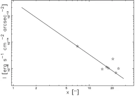
The flux of observed radiation along the centre of the jet, Ic is assumed to scale
as
(
)
(
0 0)
0 0 2
; , , ,
; , , , ,
c
Q x x v b I x x v b
x
∝
(52)
where Q, the radiative losses, is given by Equation (33). The explicit form of this equation is
(
)
(
(
)
)
(
(
)
)
2 2 3
0 0 0 0
0 0 2
1 tan 2
1
; , , , .
2
c
x x x v
I x x v b
x
α
ρ
− + − π
= −
(53)
This relation connects the observed intensity of radiation with the rate of energy transfer per unit area. A typical example of the jet of HH34 at 4.5 μm is reported in Figure 9.
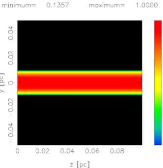
6.4. Emission from a Cylinder
A thermal model for the image is characterised by a constant temperature and density in the internal region of the cylinder. Therefore, we assume that the number density C is constant in a cylinder of radius a and then falls to 0, see the simplified transfer Equation (51). The line of sight when the observer is situated at the infinity of the x-axis and the cylinder’s axis is in the perpendicular position is the locus parallel to the x-axis, which crosses the position y in a Cartesian x-y plane and terminates at the external circle of radius a. A similar treatment for the sphere is given in [24]. The length of this locus in the optically thin layer approximation is
(
2 2)
2 ; 0 .
ab
l = × a −y ≤ <y a (54)
The number density Cm is constant in the circle of radius a and therefore the
[image:13.595.261.488.519.680.2]intensity of the radiation is
DOI: 10.4236/ijaa.2019.93022 315 International Journal of Astronomy and Astrophysics
(
2 2)
0a m 2 ; 0 .
I =C × × a −y ≤ <y a (55)
A typical example of this cut is reported in Figure 10 and the intensity of all the cylinder is reported in Figure 11.
6.5. Numerical Image
The numerical algorithm that allows us to build a complex image in the optically thin layer approximation is now outlined.
An empty, value = 0, memory grid
(
i j k, ,)
which contains 4003 pixels isconsidered.
The points which fill the jet in a uniform way to simulate the constant density in the emitting particles are inserted, value = 1, in
(
i j k, ,)
[image:14.595.232.519.294.499.2] Each point of
(
i j k, ,)
has spatial coordinates x y z, , which can be represented by the following 1 3× matrix, A,Figure 10. 1D cut of the intensity, I, when a=0.01 pc.
[image:14.595.293.460.534.706.2]DOI: 10.4236/ijaa.2019.93022 316 International Journal of Astronomy and Astrophysics .
x
A y
z =
(56)
The orientation of the object is characterised by the Euler angles
(
Φ Θ Ψ, ,)
and therefore by a total 3 3× rotation matrix, E, see [21]. The matrix point is represented by the following 1 3× matrix, B,.
B E A= ⋅ (57)
The intensity 2D map is obtained by summing the points of the rotated images.
[image:15.595.285.464.256.431.2]A typical result of the simulation is reported in Figure 12, which should be compared with the observed image as given by Figure 13.
Figure 12. 2D intensity map of HH34, parameters as in Figure 8.
[image:15.595.279.471.461.703.2]DOI: 10.4236/ijaa.2019.93022 317 International Journal of Astronomy and Astrophysics
6.6. The Mathematical Knots
The trefoil knot is defined by the following parametric equations:
( )
( )
sin 2sin 2
x= t + t (58)
( )
( )
cos 2cos 2
y= t − t (59)
( )
sin 3
z= − t (60)
with 0≤ ≤ πt 2 . The visual image depends on the Euler angles, see Figure 14. The image in the optically thin layer approximation can be obtained by the numerical method developed in Section 6.5 and is reported in Figure 15.
[image:16.595.280.468.261.437.2]This 2D map in the theoretical intensity of emission shows an enhancement where two mathematical knots apparently intersect.
Figure 14. 3D view of the trefoil when the three Eulerian angles which characterise the point of view are Φ =0, Θ =90 and Ψ =0.
[image:16.595.273.479.486.695.2]DOI: 10.4236/ijaa.2019.93022 318 International Journal of Astronomy and Astrophysics
7. Conclusions
Laws of motion:
We analysed two simple models for the law of motion in HH objects as given by the Stoke’s and Newton’s behaviour, see Section 3. A third law of motion is used for turbulent jets in the presence of a medium whose density decreases with a power law, as given by Equation (23). The model that is adopted for the turbulent jets conserves the flux of energy. For example, Equation (25) reports the velocity as function of the position. The
χ
2 analysis for observed theo-retical velocity as function of time/space, see Table 2, assigns the smaller value to the turbulent jet.
Back reaction:
The insertion of the back reaction in the equation of motion allows us to introduce a finite rather than infinite jet’s length, see Equation (39).
The extended region:
The extended region of HH34 is modeled by combining the decreasing jet’s velocity with the constant velocity and precession of the central object, see the final matrix (45).
The theory of the image:
We have analysed the case of an optically thin layer approximation to provide an explanation for the so called “bow shock” that is visible in HH34. This effect can be reproduced when two emitting regions apparently intersect on the plane of the sky, see the numerical simulation as given by Figure 12. This curious effect of enhancement in the intensity of emission can easily be reproduced when the image theory is applied to the mathematical knots, see the example of the trefoil in Figure 15.
Acknowledgements
Credit for Figure 13 is given to ESO.
Conflicts of Interest
The author declares no conflicts of interest regarding the publication of this pa-per.
References
[1] Herbig, G.H. (1950) The Spectrum of the Nebulosity Surrounding T Tauri. The As-trophysical Journal,111, 11-14.https://doi.org/10.1086/145232
[2] Haro, G. (1952) Herbig’s Nebulous Objects near NGC 1999. The Astrophysical Journal,115, 572-573.https://doi.org/10.1086/145576
[3] Raga, A.C., Reipurth, B. and Noriega-Crespo, A. (2019) The HH34 Jet/Counterjet System at 1.5 and 4.5 μm. Revista Mexicana de Astronomia y Astrofisica, 55, 117-123.https://doi.org/10.22201/ia.01851101p.2019.55.01.12
DOI: 10.4236/ijaa.2019.93022 319 International Journal of Astronomy and Astrophysics [5] Raga, A.C., Noriega-Crespo, A., Carey, S.J. and Arce, H.G. (2013) Proper Motions
of Young Stellar Outflows in the Mid-Infrared with Spitzer (IRAC). I. The NGC 1333 Region. Astronomical Journal,145, 28.
https://doi.org/10.1088/0004-6256/145/2/28
[6] Noriega-Crespo, A., Raga, A.C., Moro-Martn, A., Flagey, N. and Carey, S.J. (2014) Proper Motions of Young Stellar Outflows in the Mid-Infrared with Spitzer II HH 377/Cep E. New Journal of Physics, 16, Article ID: 105008.
https://doi.org/10.1088/1367-2630/16/10/105008
[7] Guzmán, A.E., Garay, G., Rodrguez, L.F., Contreras, Y., Dougados, C. and Cabrit, S. (2016) A Protostellar Jet Emanating from a Hypercompact H II Region. The Astro-physical Journal,826, Article No. 208.https://doi.org/10.3847/0004-637X/826/2/208
[8] Raga, A.C., Reipurth, B., Esquivel, A., Castellanos-Ramrez, A., Velázquez, P.F., Hernández-Martnez, L., Rodrguez-González, A., Rechy-Garca, J.S., Estrella-Trujillo, D. and Bally, J. (2017) Proper Motions of the HH 1 Jet. Revista Mexicana de Astro-nomia y Astrofisica,53, 485-495.
[9] Cabrit, S. and Raga, A. (2000) Theoretical Interpretation of the Apparent Decelera-tion in the HH 34 Super Jet. Astronomy & Astrophysics,354, 667-673.
[10] López-Martn, L., Raga, A.C., López, J.A. and Meaburn, J. (2001) Theory and Ob-servations of a Jet in the σ Orionis Region: HH 444. Revista Mexicana de Astrono-mia y Astrofisica Conference Series, 10, 61-64.
[11] Viti, S., Girart, J.M., Garrod, R., Williams, D.A. and Estalella, R. (2003) The Mole-cular Condensations Ahead of Herbig-Haro Objects. II. A Theoretical Investigation of the HH 2 Condensation. Astronomy & Astrophysics,399, 187-195.
https://doi.org/10.1051/0004-6361:20021745
[12] Raga, A.C., Reipurth, B., Cantó, J., Sierra-Flores, M.M. and Guzmán, M.V. (2011) An Overview of the Observational and Theoretical Studies of HH 1 and 2. Revista Mexicana de Astronomia y Astrofisica,47, 425-437.
[13] Kwon, J., Choi, M., Pak, S., Kandori, R., Tamura, M., Nagata, T. and Sato, S. (2010) Magnetic Field Structure of the HH 1-2 Region: Near-Infrared Polarimetry of Point-Like Sources. The Astrophysical Journal,708, 758-769.
https://doi.org/10.1088/0004-637X/708/1/758
[14] Lee, C.F., Rao, R., Ching, T.C., Lai, S.P., Hirano, N., Ho, P.T.P. and Hwang, H.C. (2014) Magnetic Field Structure in the Flattened Envelope and Jet in the Young Protostellar System HH 211. The Astrophysical Journal,797, L9.
https://doi.org/10.1088/2041-8205/797/1/L9
[15] Lee, C.F., Hwang, H.C. and Li, Z.Y. (2016) Angular Momentum Loss in the Envelope-Disk Transition Region of the HH 111 Protostellar System: Evidence for Magnetic Braking? The Astrophysical Journal,826, Article No. 213.
https://doi.org/10.3847/0004-637X/826/2/213
[16] De Young, D.S. (2002) The Physics of Extragalactic Radio Sources. University of Chicago Press, Chicago.
[17] Zaninetti, L. (2016) Classical and Relativistic Flux of Energy Conservation in As-trophysical Jets. Journal of High Energy Physics, Gravitation and Cosmology, 2, 41-56.https://doi.org/10.4236/jhepgc.2016.21005
[18] Zaninetti, L. (2018) Classical and Relativistic Evolution of an Extra-Galactic Jet with Back-Reaction. Galaxies, 27, 134.https://doi.org/10.3390/galaxies6040134
[19] Bally, J. and Devine, D. (1994) A Parsec-Scale “Superjet” and Quasi-Periodic Struc-ture in the HH 34 Outflow? The Astrophysical Journal,428, L65.
DOI: 10.4236/ijaa.2019.93022 320 International Journal of Astronomy and Astrophysics [20] Zaninetti, L. (2010) The Physics of Turbulent and Dynamically Unstable
Her-big-Haro Jets. Astrophysics and Space Science,326, 249-262.
https://doi.org/10.1007/s10509-009-0255-8
[21] Goldstein, H., Poole, C. and Safko, J. (2002) Classical Mechanics. Addison-Wesley, San Francisco.
[22] Rybicki, G. and Lightman, A. (1991) Radiative Processes in Astrophysics. Wi-ley-Interscience, New-York.
[23] Hjellming, R.M. (1988) Radio Stars IN Galactic and Extragalactic Radio Astronomy. Springer-Verlag, New York.https://doi.org/10.1007/978-1-4612-3936-9_9