Munich Personal RePEc Archive
Aggregation with Cournot competition:
the Le Chatelier Samuelson principle
Koebel, Bertrand and François, Laisney
9 December 2014
Online at
https://mpra.ub.uni-muenchen.de/60476/
Aggregation with Cournot competition:
the Le Chatelier Samuelson principle
Bertrand Koebel∗ and François Laisney∗∗
December 2014
Abstract. This paper studies the aggregate substitution and expansion effects
triggered by changes in input prices in a context where firms supply a homoge-neous commodity and compete in quantities à la Cournot. We derive a sufficient condition for the existence of a Cournot equilibrium and show that this condition also ensures that the Le Chatelier-Samuelson principle is satisfied in the aggregate at the Cournot equilibrium, although it may not be satisfied at the firm level.
Keywords: Aggregation, returns to scale, market power, markup, own-price elas-ticity.
JEL Classification: D21, D43.
∗ Corresponding author: Beta, UMR 7522 CNRS, Université de Strasbourg, 61 avenue de la Forêt Noire, 67085 Strasbourg Cedex (France), [email protected].
∗∗Beta, UMR 7522 CNRS, Université de Strasbourg, and ZEW Mannheim,fl[email protected].
1. Introduction
This paper investigates the consequences of input price changes on input demands when
the output market is imperfectly competitive. The impact of input price changes on
input adjustment is described by the Le Chatelier principle, introduced in economics
by Samuelson (1947). This principle states that the sensitivity of input demands with
respect to own price variations is smaller when the output level is held constant than
when it is adjusted. It is apparently not widely known, however, that Samuelson (1947,
p.45-46) showed that the Le Chatelier principle is satisfied whether competition on the
output market is perfect or imperfect, provided the production level of competitors is
held constant. At the firm level, the Le Chatelier principle attracted the attention
of many researchers who derived it by weakening or changing underlying assumptions
(see e.g. Eichhorn and Oettli, 1972, Diewert, 1981, and Milgrom and Roberts, 1996).
However, these authors did not consider whether the principle is still satisfied when
negative externalities between firms affect their behavior. The aim of this paper is to
fill this gap in the literature and to extend the Le Chatelier-Samuelson (LCS) principle to the case of Cournot competition with endogenous levels of competitors’ output.
For a given level of output, a cost minimizing firm has an incentive to use more
in-tensively the input whose price has decreased and to substitute the cheaper one for the
other inputs (the substitution effect). When the firm is less constrained and becomes
able to set its output level in order to maximize its profit, it will choose the optimal
output level in order to benefit even further from the input price reduction. This
adjust-ment corresponds to an expansion effect. In a competitive output market this expansion
effect is always negative, because firms do not consider that the aggregate increase in output induces a drop in the output price. With imperfect competitive output markets
à la Cournot, the sign of the expansion effect is ambiguous, because the externality
provides incentives to reduce input demand: if all competing firms increase their output
level in order to exploit the reduction in input price, the output price must fall, and this
reduces each firm’s incentives to expand its level of output supply and input demand.
Firm level comparative statics are therefore undetermined. Only further restrictions on
make it possible to obtain well-determined results.
In this paper we show that, despite ambiguous results at the firm level, under
Novshek’s (1985) type of conditions (which ensure the existence of a Cournot
equi-librium), the aggregate expansion effect is negative and the LCS principle is valid in the
aggregate Cournot model. The existing literature deriving comparative static results for
Cournot oligopolies does not cover this paradox because it investigates comparative
sta-tics at the firm level (Dixit, 1986, Hoernig, 2003). We show that aggregation is helpful
for resolving the ambiguity at the firm level.
This result can in turn be applied to study the aggregate impact of taxes, subsidies, or,
more generally, shocks affecting aggregate demand or firm’s cost functions. When firms
are heterogenous with respect to their size and technologies, identical and symmetric
demand shocks affect them differently: the input demands of smaller firms may shrink
while those of bigger firms increase. A related issue has, for instance, been studied by
Février and Linnemer (2004) who consider the impact of a cost shock on aggregate profits
and welfare. Our paper focuses on input demands, and shows that despite heterogenous
reactions at the micro level, the aggregate reaction is well determined.
The next section outlines the microeconomic model and derives the LCS principle at
the firm level, when the output market is imperfectly competitive. Section 3 exposes
Novshek’s (1985) sufficient conditions for the existence of a Cournot equilibrium. Section 4 extends the LCS principle to the case of Cournot competition at the aggregate level,
it also describes the aggregate consequences of Cournot competition in terms of input
adjustment. Section 5 concludes.
2. Input demands with Cournot competition
The model is developed at the microeconomic level of the production unit. Vector
∈ R+ denotes input quantities and is the corresponding ×1 price vector. The
production unit’s output level is denoted by ∈ R+ Under suitable regularity
condi-tions the technology of a cost minimizing production unit is fully described by a twice
continuously differentiable cost function By definition,( ) =|∗( ) where∗
input demands react to input prices, at the level of the firm.
In an imperfectly competitive product market, the production unit knows the inverse
product demand function : 7→() it faces. Let − denote the production level of
all competitors to firm . The profit function is given by
( −) = max
{(+−)−( )} (1)
= (+−)−( ) (2)
where ( −) denotes the optimal solution to (1) and represents the output supply
correspondence. One difficulty with is that it is not necessarily a function since for some values of ( −) there might be several profit-maximizing output supplies. In the following we assume that the solution is locally unique. At this point we should emphasize that our analysis is purely local, i.e. we consider only small changes in input
prices.
Let 0 and 00 denote the first and second derivatives of function The first order
condition for an interior optimum is given by
(+−) +0(+−) =
¡ ¢
(3)
Output supply changes when the demand function shifts (variation in −) or when the cost parameters change.
Some authors — reviewed by Appelbaum (1982) and Bresnahan (1989) — consider that
this simple framework encompasses a variety of non-competitive pricing behaviors. In
this section, we follow the Cournot-Nash conjecture and consider the production level of
competitors as fixed whilefirm is choosing its optimal production level. Note that−
is specific to firm A sufficient condition for an interior maximum is that, in addition
to (3),
( −)0 (4) with
( −)≡
∙
20(+−) +00(+−)−
2
2
( ) ¸−1
(5)
Inequality (4) can be fulfilled even in the case of decreasing marginal costs (2
2
By Hotelling’s lemma the input demand functions are given by:
( −) =−
( −) =
(
( −)) =∗( ( −)) (6)
where the second equality follows from (3).1 Thus, just as in the perfect competition
case, the constant-output and the unrestricted input demand functions coincide at the
optimal output level. Concerning comparative statics, the × matrix of the partial
derivatives of the column vector of input demands w.r.t. the row vector of input prices | can be expressed as:
|( −) =
∗ |(
) +
∗ (
( −))
| ( −)
= ∗
|(
) +( −)
∗ (
)
∗| (
) (7)
where the second equality follows from the differentiation of (3) with respect to
yielding:
( −) =
( −)
∗ (
) (8)
This allows to obtain the LCS principle in imperfect competition.
Proposition 1. Assuming ( −)0
(i) the LCS result is satisfied:
( −)≤ ∗
( )0 (9)
(ii) an increase in input price decreases the output level iff input demand ∗ is
normal:
0⇔∗ 0 (10)
(iii)an increase in input priceincreases the output price( −)≡¡( −) +−¢
if output demand is decreasing and ∗ is normal:
©
0()0∧∗ 0ª⇒ 0 (11)
Statement (i) directly follows from (7), (ii) from (8) and (iii) from the inverse
de-mand function and (8). This result shows how increases in input prices reduce input
demand, which in turn decreases production and creates inflation. Part (i) of
sition 1 is satisfied without requiring input demand to be normal.2 The conditions
(( −) 0 ∗ 0 and 0 0) necessary for obtaining statements (ii) and
(iii) of Proposition 1 can be investigated empirically. Note that the comparative static
statement of Proposition 1 assumes that − is exogenous.
Samuelson (1947, p.45-46) derived this principle using a revenue function noted()
which is compatible with a perfectly competitive output market, when () = ()
but also with imperfect competition for () = (() +−)() A more general formulation of the Le Chatelier principle, yielding Proposition 1(i) as a special case,
was provided by Eichhorn and Oettli (1972). In comparison to Samuelson’s result, the
above derivation of the LCS principle has the advantage of relying on the dual: it yields
thereby Equation (7) which resembles the Slutsky decomposition in consumer theory.
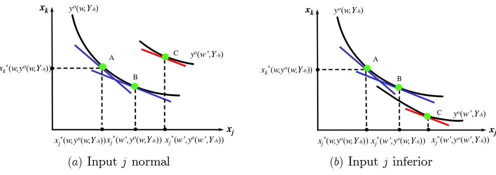
Figure 1 illustrates the optimal adjustment of output and its implication for the
inputs. This figure, presented by Sakai (1973) in the competitive setup, is also valid
when production functions are not concave and production units have market power,
as long as − is constant. The shift from point to point along the isoquant
corresponding to production level ( −) represents input substitution caused by a
decrease in the price of input from to 0. The shift from to arises when the
production unit chooses the profit-maximizing output level, and depicts the expansion
(or scale) effect. For normal inputs, this expansion effect is positive and by (8) it turns out that in this case the production unit increases output to its optimal level(0
−).
When input is inferior, the converse applies (see Figure 1b): profit is maximized when
the firm decreases output after the decrease of (see 10). Figure 1 illustrates that in
both cases the unrestricted move in the input demand from( −)to (0
−)
will be larger than the restricted move from ( −) to ∗(0 (
−)) The LCS
principle differs from the Slutsky decomposition because production units maximize
profit and not production: in the situation of Figure 1b, profits are maximized by
reducing production.
2
xj xj*(w,yo(w,Y-h))
xk yo(w,Y-h)
A
B
yo(w’,Y-h)
xj*(w’,yo(w,Y-h))xj*(w’,yo(w’,Y-h))
xk*(w,yo(w,Y-h))
C
xj xk yo(w,Y-h)
A
B
yo(w’,Y-h)
C xk*(w,yo(w,Y-h))
xj*(w,yo(w,Y-h))xj*(w’,yo(w,Y-h)) xj*(w’,yo(w’,Y-h))
[image:8.595.69.565.63.238.2]() Input normal () Input inferior
Figure 1: Substitution and expansion effects and input adjustment
There are alternative sets of assumptions which yield the conclusions of Proposition
1 (see Milgrom and Roberts, 1996). However, as our objective is to identify both the
substitution and scale effects of (7) we rely mainly on duality theory.
In terms of elasticities, (9) becomes
¡;¢≤¡∗;¢0 (12)
where
¡;¢≡
( −)
( −)
The own-price elasticities of profit-maximizing input demands are smaller than those
derived from cost-minimizing input demands. The economic intuition behind this result
is that when the output level can be adjusted after a decrease in input price , this
change in scale is made in such a way as to fully benefit from the input price reduction,
which is achieved by increasing (and if is normal). Note that input demands are
not required to be normal (that is, increasing in the level of output) to obtain the LCS
principle.
3. Existence of a Cournot-Nash equilibrium
Changes in input prices affect all firms simultaneously, which in turn affects the inverse
output demand function through changes in −. Therefore the result in the former section (derived for constant −) only partly describes the consequences of changes in
input prices. We consider an industry that can be relatively well described as a market
with respect to their cost function, their market power and their market share, measured
by In contrast to the contestable market literature, we do not require that all (potential) firms have access to the same technology.
When products within an industry are perfectly substitutable, all activefirms charge
or face the same price at equilibrium. The number of incumbent firms is exogenous.
In this setup, some firms make positive profits because they are able to produce more
cheaply than others as their technology is more efficient.
In this section we consider strategic interactions between firms and describe their
influence on input-demand adjustments. A look at the reaction functions ( −)
( −) suffices to see that strategic interactions have an important impact on the output and input demand choices. Using (3) and (5), it can be verified that the sign
of − is the same as that of 0+
00 and for this reason the Cournot game can
exhibit a nonmonotone best response, including strategic substitution (− ≤ 0) and complementarity (− ≥0).
A Cournot equilibrium is any -tuple () and () such that, for any active
firm, (3) and (4) are satisfied and the product market is cleared. So, at a Cournot equilibrium,
() =³ −()´ () =∗³ ()´=³ −()´ (13)
If we assume that is a continuous function in − for every , then Brouwer’s fixed
point theorem can usually be applied to show that a Cournot equilibrium exists.
How-ever, in Cournot oligopolistic markets, it is restrictive to assume that is a continuous function, because the profit function is not necessarily concave in for all values of
( − ) Several economists have tried to get around the assumption of concave profits to prove the existence of a Cournot equilibrium.
Novshek (1985) has shown that a -firm Cournot equilibrium exists provided that a
“firm’s marginal revenue be everywhere a declining function of the aggregate output of
others”, that is:
function is linear or concave in , in which case the existence of a Cournot equilibrium
is guaranteed. Since this condition has to be satisfied for any value of and−it can equivalently be written as
0() + 00()≤0 (15)
for any This inequality depends on aggregate data only and implies that condition
(14) is fulfilled forany firm.3
There are two difficulties with this aggregate condition. On the one hand (15) is
sufficient for the existence of a Cournot equilibrium, but not necessary, and is therefore not the weakest possible condition for achieving existence. On the other hand, the fact
that (14) has to be satisfied for any value of and − is very demanding. It must even be satisfied for the case in which one firm produces the total output, which could
reasonably be excluded if there is a competition law enforcing an upper bound for the
market share, or alternatively, if the firms’ cost functions lead them to always choose
an output level which is smaller than We thereforefirst derive a new condition which
ensures the existence of a Cournot equilibrium.
Proposition 2. Assume that for any firm, there is a maximal capacity so that no
firm chooses . If
0() +00() ≤0 (16) for any 0≤ ≤ then a Cournot equilibrium exists.
Proposition 2 is a reformulation of Novshek’s (1985) Theorem 3.4 The assumption
≤ implies that aggregate output is bounded from above by The proof of Proposition 2 follows from the fact that the output space [0 ] is a complete lattice, and imposing to be included in the interval [0 ] still yields a reaction correspondence
that is nonincreasing in− just as in Novshek’s case. Thefirst interesting consequence of Proposition 2 is that we can derive a simple and testable aggregate condition, which
implies that (16) is satisfied for any firm, and which is weaker than condition (15)
obtained by Novshek (in some sense, see footnote 4). Condition (16) is trivially valid if
3 Amir (1996) provided an alternative sufficient condition ensuring the existence of Cournot’s equilibrium. This
con-dition is discussed and empirically investigated by Koebel and Laisney (2012).
4 The new requirement thatfirm’s choice is bounded above,
≤, is weaker than Novshek’s condition∃ := 0, but in the absence of a regulatory authority (instead of a maximum capacity,can be interpreted as afirm’s maximum output level that a competition commission tolerates in this oligopoly market), the condition≤puts restrictions on
00≤0 since 0≤0. If00 0 then (16) is implied by the aggregate condition
0() +00()√H≤0 (17) for any aggregate and elementary output levels ≤ and ≤ compatible with the
Hirschman-Herfindahl index of concentration H. This is because the highest possible
market share satisfies ≤ √H and so ≤ ≤ √H for any Provided the restriction on the distribution of output is valid (≤), condition (17) is weaker than
(15), in the sense that for a given value of it is satisfied for a broader set of values for
0 and 00 than (15).
4. Aggregate comparative statics
Firm level comparative statics have been studied by Roy and Sabarwal (2008, 2010) who
derive conditions ensuring monotone comparative statics at the firm level in games with
strategic substitutes. In Section 2 (Proposition 1), we show that the LCS principle is
satisfied at thefirm level for a given level of the aggregate production of all competitors.
At a Cournot equilibrium, however, the total impact of a change in input prices follows
from (13):
() =
³
−()´+
− −
() (18)
() = ∗
³
()´+ ∗
() (19)
= ∗
³
()´+ ∗
³
−()´+ ∗
−
− ()
Even if 0(see Proposition 1(ii)) we cannot be sure that ≤0unless the last term in (18), corresponding to a change infirm’s output triggered by the strategic
interaction with all other firms, does not outweigh the direct impact of an increase in
As this last term can be positive or negative, the overall sign ofis undetermined. The same remark applies to (19) since a further and indeterminate “externality-induced
input adjustment” is added to the substitution and expansion effects of (7) and this
explains why the LCS principle is not necessarily satisfied at the firm level. It will now
be interesting to analyze whether the LCS principle holds at the aggregate level of the
4.1
Cournot equilibrium
We show that the LCS principle is satisfied in the aggregate, provided some additional
and plausible regularity conditions hold. Let us define the aggregate input demand
functions ∗ for fixed levels of individual production as:
∗³{}=1´≡
X
=1
∗( )
Similarly, let () and () denote the aggregate Nash equilibrium outcome. We are now able to describe how these aggregate quantities vary with (see the Appendix
for a proof).
Proposition 3. The impact of a change in on the Cournot equilibrium aggregate
quantities is given by:
() = () X ()∗ ³
()´ (20)
> () =
∗ |
µ
n()o
=1 ¶ (21) + X ()∗ ³ ()´ ∗| ³ ()´ +() X
()³0³()´+00³()´()´∗
³ ()´ X ∗ > ³ ()´ where () ≡ ∙
0³ ()´−
2 2 ³ ()´¸ −1 (22) () ≡ " 1 + X
³0³()´+00³()´()´ #−1
(23)
The three matrices involved in the LCS decomposition (21) have an interesting
inter-pretation: the first corresponds to the impact of on keeping all individual output levels constant; the second matrix represents the impact on due to the adjustment of the individual output levels; and the third matrix describes the consequence of the
contributions to oligopoly theory:5
()0 (24)
then, together with (14), it turns out that
()0 (25)
These inequalities place some structure on (20)-(21) and guarantee that the second
ma-trix on the RHS of (21) is negative semidefinite so that the determinateness of>
depends on the third matrix.
Corollary 1. Assume that inequalities (4), (16), and (24) are satisfied at the Cournot
equilibrium, and that either
(i) all firms are in a symmetric Nash equilibrium for any value of ,
(ii) all firms exhibit normal input demand functions ∗,6
(iii) the output demand function is linear.
Then the own-price elasticity of aggregate input demand is greater (in absolute value)
than for fixed levels of outputs:
³;
´
≤¡∗;¢≤0 (26)
Note that conditions (i)-(iii) of Corollary 1 are not equivalent (Example 1 below
illustrates that(ii) and(iii) together do not imply(i)). Corollary 1 gives three sufficient conditions which ensure that the last matrix of (21) is negative semidefinite. It is
important to note that it is actually not necessary for the third matrix on the RHS of
(21) to be negative semidefinite for obtaining (26).
As a referee pointed out, condition (i) is too specific to be interesting since under
symmetry, individual comparative statics are determinate if and only if aggregate
com-parative statics are determinate. Condition (ii) introduces the assumption of normal
input demands, and relaxes the restriction on heterogeneity. It is compatible with
a wide variety of heterogenous technologies, for instance, any homothetic production
function is appropriate. If = (()) where is homogeneous of degree one
5 See for instance Szidarovszky and Yakowitz (1977), or Vives (1999, p.99). 6
It can be shown that condition(ii)also implies that the elasticity of aggregate output with respect to the input price is negative,;
and is strictly increasing, then the cost and input demand functions take the form
( ) = ()−1() and ∗( ) = ()−1() with () ≡ () Con-dition (ii) guarantees that ≤ 0 and ∗ ≥ 0 for any firm, in which case
the LCS principle is satisfied at the micro level by (19) and, as a consequence, also in
the aggregate. Condition (ii) also implies that the elasticity of aggregate output with
respect to the input price is negative, ¡;¢≤0
The assumptions underlying this corollary are quite strong, and can be rejectedprima
facie. However, Proposition 3 shows that the LCS principle is more generally valid in
the aggregate, without requiring the strong restrictions given in the above corollary. We
therefore have good reasons to expect that aggregate input and output are decreasing
when the price of input increases. This result is not straightforward in an imperfectly
competitive context. On the one side, a firm has an incentive to increase its own output
and input levels in reaction to decreases in its competitors’ output and input levels
following an increase in input prices: − ≤ 0 and − ≤ 0. On the other
side, naive intuition suggests that any ambiguity at the micro level should be inherited
at the macro level.
These results show that strategic interaction, more than heterogeneity, hampers
de-terminate comparative statics at the firm level and, to a lesser extent, in the aggregate.
Let us consider the case of a monopoly, which annihilates both issues of heterogeneity
and strategic interaction. Then, determinate comparative statics hold (by Proposition
1) for this monopoly. If we now aggregate several such monopolies (from disjoint
mar-kets), with technologies which can be arbitrarily different, then the aggregate input demand for these monopolies still obeys the LCS principle, because there is no strategic
interation between them, and adding up nonincreasing functions yields a nonincreasing
aggregate function. Heterogeneity is therefore not the source of the problem, but rather
the strength of strategic interaction. In the competitive case, Heiner (1982) showed
the validity of the LCS principle when the output price adjusts to clear the market,
without requiring any restriction on individual technologies (see Section 4.2 below for a
discussion).
The following example illustrates why the LCS can be valid in the aggregate without
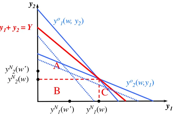
Example 1. In a standard Cournot duopoly with linear inverse demand = −
(1+2) and cost function ( ) =(), the reaction functions are given by:
( −) = −−−()
2
and the Cournot equilibrium is:
= −2() +−()
3
What happens when increases? At the firm level the impact on is undetermined, but at the aggregate level, the impact is negative, because:
() = 2−1()−2() 3
decreases when increases (since is increasing in ). This example is a special case of Corollary 1(ii) and (iii) as both firms have a technology with constant returns to
scale and output demand is linear.
y
1y
1+ y
2= Y
y
2y
o2
(
w,y
1)
A
y
o1
(
w, y
2)
B
C
y
N 1(
w
)
y
N2
(
w
)
y
N 1(
w’
)
y
N [image:15.595.150.454.355.557.2]2
(
w’
)
Figure 2: Comparative statics at thefirm level and in the aggregate
The reaction curves and Nash equilibria are depicted in Figure 2. This figure also
includes the iso-output line 1+2 = going through the aggregate Nash equilibrium
Any point below this line corresponds to a smaller aggregate output level than
triangle A the output level of firm 2 increases and the output of firm 1 decreases. In
rectangle B the output levels of bothfirms decrease, and in triangle C the output levels
of both firms go in opposite directions. In all three cases, however, the total output
level 1 +2 decreases after a price increase from to 0
Note that the result depicted in Figure 2 does not decisively depend upon the slope
of the reaction function as such a figure can also be obtained for both increasing in
− or when one reaction function is increasing and the other decreasing in −. The important ingredient for obtaining the aggregate comparative statics result is that at
least one reaction function is shifted downwards after an increase inwhich is ensured
if ∗ is normal (see Proposition 1(ii)).7
Since in Example 1, micro input demands ∗( ) are proportional to a similar
figure can be drawn in the (1 2) coordinate plane. Regarding aggregate inputs, we
can write (21) as follows:
() = ∗
³
1() 2()´−1
2
X
=1
µ∗
³
()´
2
− 3
à 2 X
=1
1
∗
³
()´ !2
All three terms on the RHS of the equality are negative, and the LCS principle holds.¤
y
1y
1+ y
2= Y
y
2y
o2
(
w,y
1)
y
o1
(
w, y
2)
y
N 1(
w
)
y
N 2(
w
)
y
N 1(
w’
)
[image:16.595.119.526.427.673.2]y
N 2(
w’
)
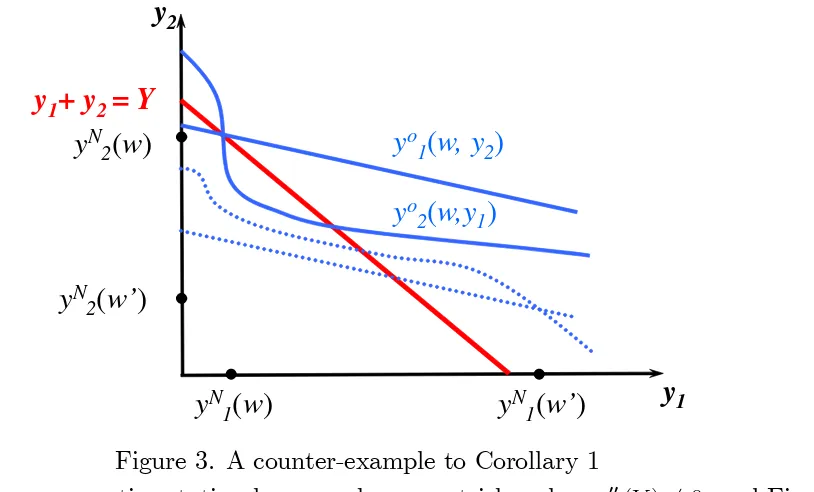
Figure 3. A counter-example to Corollary 1
Aggregate comparative statics, however, becomes tricky when 00()6= 0, and Figure
3 illustrates that the claim of Corollary 1 can be violated in these nonlinear cases. This
7 The result can still be satis
counter-example works because both reaction curves 1 and 2 cross the iso-aggregate output line1+2= afterincreases to0. In this counterexample the market shares
of both firms are drastically shifted by a marginal change in, which is empirically not
often observed.
There are three reasons why inequalities (26) can be violated at a Cournot
equilib-rium. First, a Cournot equilibrium can exist even if (14) or (17) is violated, in which
case ³;
´
may become positive. However, the validity of (17) can be investigated
empirically. In the case where (17) cannot be rejected, this provides evidence both for
the existence of a Cournot equilibrium and for the validity of the aggregate LCS
prin-ciple. Nonnormal input demands represent a second source of violation. Third, with
multiple equilibria, large shocks on can shift the economy from one Nash equilibrium
to the other. However, as clearly emphasized, the above analysis is only valid locally
around the initial equilibrium.
These results and figures help understand why some firms with market power (like
recently Deutsche Post in Germany) are pushing trade-unions and the government to
increase (or introduce) a minimum wage. The resulting increase in labor cost for the
lobbying firm can be compensated by an increase in its market share (and even profits)
because it hurts the competitors more than the firm itself.
It is of course possible tofind weaker sufficient conditions than those given in Corollary 1, at the cost however of being economically less intuitive to interprete. One possibility is
to make a plausible assumption on average input demand sensitivity w.r.t. output. For
instance, assuming that P ¡0+00 ¢∗ is positive and that P ∗ is a negative vector also yields the aggregate LCS principle and this assumption is clearly
weaker than Corollary 1(ii).
4.2
Input demand reactivity and degree of competition
In order to better understand the role played by imperfect competition in obtaining the
results above, let us compare the Cournot outcome with the benchmark of a market
where all firms are in perfect competition. This case was studied by Heiner (1982) and
Braulke (1984). We present an alternative derivation of their main result and compare
In perfect competition, the price level is exogenous at the level of production unit
and the profit maximising output supply ( ) satifies
=
( ( )) (27)
with
( )≡
∙
−
2
2
( ( )) ¸−1
0 (28)
The aggregate product supply ( )is related to the profit-maximising output supplies
(27) by ( )≡P=1( )The competitive output price level()is the solution
in to the market clearing condition:
=¡ ( )¢ (29)
where still represents the inverse demand function. The corresponding microeconomic
and aggregate competitive equilibrium output levels are denoted by
() = (() ) (30)
() = (() ) =
X
() (31)
Similarly, the microeconomic and aggregate equilibrium input quantities are given by
() ≡ ∗( ()) (32)
() ≡
X
() (33)
If we evaluate (27) at the equilibrium price = () and differentiate w.r.t. we obtain:
() =(
() )µ∗
(
())−0(())
|()
(34)
which can be compared with (39) in imperfect competition.
Whereas at the microeconomic level it is not possible to say how ()or()vary with because the output-price response effect is indeterminate, Heiner (1982) and
Braulke (1984) have shown that this effect is well determined in the aggregate. “This reassuring effect [...] represents one of the few cases where an ambiguity at the micro
level is resolved at the macro level by aggregation” (Braulke, 1984, p.75). Summing up
(34) over all firms yields the aggregate impact of a change of input price on output:
=
à 1 +0
X
!−1
X
Although the sign of is indeterminate (unless one assumes that input demands are normal), the aggregate impact of input prices on input demands is well determined
and given by
| () = X ∗ |( ()) + X ∗ ( ())
|() (35)
= ∗
|
³
{}=1´+
X ∗ ∗| + 0
1 +0P
" X ∗
# " X ∗ #>
Thefirst equality is a consequence of identity (32), the second equality is obtained after
substituting | into the expression of
|. The last term on the RHS
corre-sponds to the adjustement of output price and is negative semidefinite. Altogether we have shown that with perfect competition on the output market:
| ()¿
∗ |
³
{}=1´¿0 (36) These inequalities mean that in the aggregate, output quantity and price adjustment
amplify the shock in input prices on∗, and the reactions in aggregate input quantities then become more important than for constant output and price level. With perfect
competition, no restrictions on firms’ heterogeneity (technology or production level) is
necessary to obtain monotone comparative statics in the aggregate.
How do the non-competitive aggregate input reactions > compare to the corresponding matrix > obtained with a perfect competitive output market?
Some authors, like Cahuc and Zylberberg (2004, p.186) rely on (7) in order to argue
that the expansion effect "diminishes in absolute terms" when market power rises. This
claim is true ceteris paribus, that is, when the technology is independent from market
power, but it is not necessarily satisfied otherwise. As a consequence, their conjecture
will not necessarily be satisfied at the aggregate level of an industry, where the link
between the degree of competition and the size of the expansion effect becomes an
empirical issue. This quantification is the purpose of the companion paper Koebel and
Laisney (2013).
In summary, this subsection shows that competitive output markets do not necessarily
5. Conclusion
Output adjustments have important consequences on input demands. This impact,
however, is rarely considered in economic contributions, because with imperfectly
com-petitive output markets, increasing returns to scale and externalities disturb the usual
representative firm’s comparative statics. This paper derives the circumstances under
which the LCS principle holds in an aggregate Cournot economy with heterogenous
firms.
Whereas at the firm level the impact of changes in the input price on output supply
and input demand is ambiguous, aggregation over firms belonging to the same industry
has a regularizing effect. We show that when a Cournot equilibrium exists, then aggre-gate input demand is decreasing in the price of this input under plausible conditions.
In the oligopoly case, restricting heterogeneity is a way to canalise the price adjustment
effect and enforce the LCS principle in the aggregate.
6. Appendix: Proofs of results
Hotelling’s lemma with imperfect competition. We derive Equation (6) using the
definition of the profit function,
( −) =(( −) +−)( −)−( ( −))
It implies that the impact of a marginal change in input prices on profit is given by
( −) = £
0(( −) +−)( −) +(( −) +−)¤
( −)
−
(
( −))−
(
( −))
( −( −))
⇔
( −) =−
( −)
where the last line is a consequence of (3) and Shephard’s lemma, which states that cost
minimizing input demands coincide with the partial derivatives of the cost function w.r.t. .
Proof of Proposition 3.
Differentiating
³()´+0³ ()´ () = ¡
()¢
with respect to we obtain (suppressing the arguments in the result)
0
+
00
+0
=
∗ +
2
2
(38)
and it turns out that
= µ ∗ − ³
0+00 ´
(39)
Summing up (39) over allfirms yields the impact of a change of input price on aggregate
output: = Ã 1 + X
³0+00´
!−1
X ∗ = X ∗
The impact of input prices on aggregate input demands is given by
| = X ∗ | + X ∗ | = ∗ | + X ∗ ∗| + " X
³0+00 ´
∗
# "
X ∗ #> ¤
Proof of Corollary 1.
(i) When firms are in a symmetric Nash equilibrium, = for any and so the last matrix of (21) can be written as
"
X
³0+00´∗
# " X ∗ > #
= ³0+00´ "
X
∗
# " X
∗
#>
which is negative semidefinite.
(ii) When input demands are normal, ∗ 0 for any , any firm and any input
Then there exist numbers 0 such that
X
³0+00´
∗ = X ∗
In fact, this equation defines Let be a diagonal matrix with (1 )> on
the diagonal. So it turns out that
"
X
³0+00´∗
# " X ∗ #> = " X ∗
# " X ∗ #>
and all entries on the diagonal of this matrix are negative. However, the matrix itself is not negative semi-definite, as can be checked in the case = 2 when the two components of ∗coincide. With simplified notations, we look at the eigenvalues of the symmetrized matrix >+> and with = diag ( ) and > = ( ). These are 2³+−√2√2+2´ ≤ 0 and 2³++√2√2+2´ which is strictly
(iii) The proof is similar to point (i) but with 00= 0 ¤
7. References
Amir, R., 1996, “Cournot oligopoly and the theory of supermodular games,” Games and Economic Behavior, 15, 132-148.
Appelbaum, E., 1982, “The estimation of the degree of oligopoly power,” Journal of Econometrics, 19, 287-299.
Braulke, M., 1984, “The firm in short-run industry equilibrium: comment,” American Economic Review, 74, 750-753.
Bresnahan, T. F., 1989, “Empirical studies of industries with market power,” in R. Schmalensee and R. D. Willig (Editors), Handbook of Industrial Organization, Volume 2, 1011-1057.
Cahuc P. and A. Zylberberg, 2004, Labor Economics, MIT Press.
Diewert, W. E., 1981, “The elasticity of derived net supply and a generalized Le Chatelier principle’, Review of Economic Studies, 48, 63-80.
Dixit, A., 1986, “Comparative statics for oligopoly,” International Economic Review, 27, 107-122. Eichhorn, W. and W. Oettli, 1972, “A general formulation of the Le Chatelier-Samuelson Principle,”
Econometrica, 40, 711-717.
Février, P. and L. Linnemer, 2004, “Idiosyncratic shocks in an asymmetric Cournot oligopoly,” In-ternational Journal of Industrial Organization, 22, 835-848.
Heiner, R. A., 1982, “Theory of the firm in “short-run” industry equilibrium,” American Economic Review, 72, 555-62.
Hoernig, S. H., 2003, “Existence of equilibrium and comparative statics in differentiated goods Cournot oligopolies,” International Journal of Industrial Organization, 21, 989-1019.
Koebel, B. M. and F. Laisney, 2010, “The aggregate Le Chatelier Samuelson principle with Cournot competition,” ZEW Discussion Paper 10-009, Mannheim.
Koebel, B. M. and F. Laisney, 2013, “Aggregation with Cournot competition: an empirical investiga-tion,” mimeo, BETA, Université de Strasbourg.
Milgrom, P. and J., Roberts, 1996, “The Le Chatelier principle,” American Economic Review, 86, 173-179.
Novshek, W., 1985, “On the existence of Cournot equilibrium,”The Review of Economic Studies, 52, 85-98.
Roy, S. and T. Sabarwal, 2010, “Monotone comparative statics for games with strategic substitutes,” Journal of Mathematical Economics, 46, 793-806.
Roy, S. and T. Sabarwal, 2008, “On the (non-) lattice structure of the equilibrium set in games with strategic substitutes,”Economic Theory, 37, 161—169.
Sakai, Y., 1973, “An axiomatic approach to input demand theory,” International Economic Review, 14, 735-752.
Samuelson, P. A., 1947,The Foundations of Economic Analysis, Harvard University Press.
Szidarovszky, F. and S. Yakowitz, 1977, “A new proof of the existence and uniqueness of the Cournot equilibrium,”International Economic Review, 18, 787-789.