On prospects and games: an equilibrium
analysis under prospect theory
Rindone, Fabio and Greco, Salvatore and Di Gaetano, Luigi
Economic and Business, university of Catania
6 June 2013
Online at
https://mpra.ub.uni-muenchen.de/52131/
an equilibrium analysis under prospect theory
preferences
Luigi Di Gaetano
∗Salvatore Greco
†Fabio Rindone
‡Department of Economics and Business,
University of Catania, Corso Italia 55, 95129 Catania, Italy
Abstract
The aim of this paper is to introduce prospect theory in a game the-oretic framework. We address the complexity of the weighting function by restricting the object of our analysis to a 2-player 2-strategy game, in order to derive some core results. We find that dominant and indifferent strategies are preserved under prospect theory. However, in absence of dominant strategies, equilibrium may not exist depending on parameters. We also discuss a different approach presented by Metzger and Rieger (2009) and give some interesting interpretations of the two approaches.
JEL Classification: C70; D03.
Keywords: Game theory, Prospect theory, Nash equilibrium, Behavioural economics.
1
Introduction
Expected utility theory (EUT), as axiomatised by Von Neumann and Morgen-stern (1944), has represented a crucial definition in game theory. Indeed, it is a central model used both to shape rational choice in a normative way and to describe economic behaviour. However, its underlying assumptions are far from being harmless, especially when dealing with uncertainty and risk (Kahneman and Tversky, 1979).
Moreover, scholars have been debating both on the validity of the expected utility assumption, and on the likelihood of theoretical results derived under this assumption (see, for instance, Starmer, 2000). Furthermore, experiments, examples and paradoxes have been analysed, leading to results which are far from those predicted by EUT.
In the field of risk and uncertainty several models have been developed as alternative to EUT. Among these we find prospect theory (PT) and cumulative prospect theory (CPT) (Kahneman and Tversky, 1979; Tversky and Kahneman, 1992), rank dependent utility (Quiggin, 1982), and Choquet expected utility (Schmeidler, 1986, 1989; Gilboa, 1987).
∗
email: [email protected]
†email: [email protected] ‡email: [email protected]
The main reason why these alternative models have been developed is the observation of systematic violations of EUT axioms in economic behaviour (see Camerer, 1995; Schoemaker, 1982; Starmer, 2000).
Perhaps, the Allais paradox (Allais, 1953) is the most famous example of these violations. Kahneman and Tversky (1979) observe that there are system-atic errors in agent’s choice, commonly known as ‘certainty effect’, ‘reflection effect’, and ‘isolation effect’. People put a greater weight to payoffs which are certain, while they “underweight outcomes that are merely probable” (Kahne-man and Tversky, 1979). They find, furthermore, that positive outcomes are evaluated differently from negative payoffs, and people are risk averse for pos-itive values, and risk seeking when dealing with negative values (Markowitz, 1952; Kahneman and Tversky, 1979). Finally, the framework in which data are presented to agents has a determinant effect on their final choice.
From these considerations they develop a theory of prospects1
, which intro-duces several new features. In particular, outcomes should be valued as relative gains and/or losses with respect to a reference point and the marginal utility of losses is bigger that that of gains. Furthermore, agents overweight almost cer-tain events and underweight almost uncercer-tain outcomes.These features account for the three effects briefly presented above;
This paper aims at introducing prospect theory in games and defining a preliminary approach of analysis. Although the relative great success of PT and CPT in decision theory (e.g., Benartzi and Thaler, 1995; Barberis et al., 2001; Camerer, 2000; Jolls et al., 1998; McNeil et al., 1982; Quattrone and Tversky, 1988), the consequences of introductioning CPT in game theory have hardly been investigated.
To the best of our knowledge there is only one contribution on the topic (Metzger and Rieger, 2009). They define a general framework and underline the major issues in such analysis, and derive a general existence result.
If on the one hand so little has been written about prospect theory in games, on the other it is possible to refer to part of the literature which analyses – theoretically or by showing evidences – deviations from the expected utility assumption2
.
Crawford (1990) discusses the existence issue when the independence axiom of von Neumann–Morgenstern is violated. Furthermore, he defines the concept of equilibrium in beliefs and gives sufficient conditions for the existence of NE. The same issue is analysed by Dekel et al. (1991) when preferences do not satisfy the reduction of compound lottery assumption. They analyse two major issues; the first is the existence of NE, which depends on players’ perception of themselves as moving first or second. The second issue regards the dynamic consistency of strategies.
Chen and Neilson (1999) analyse pure–strategy Nash Equilibruia when pref-erences do not follow the expected utility assumption. They find that prefer-ences should be quasi–convex in probabilities. They also find that continuity
1
Kahneman and Tversky (1979) introduced PT in their seminal paper. They developed a variant of PT, called CPT, where the weighting is applied to the cumulative probability distribution function (cdf), as in rank-dependent expected utility theory. In this paper we refer to PT with regard to the basic insight of the model, while we refer to CPT for the mathematical specification of the model.
2
and first order stochastic dominance is needed to assure the equilibrium in a deterministic game.
Metzger and Rieger (2009) discuss the existence of NE within a PT frame-work, as well as the divergence from EUT equilibrium predictions. They, how-ever, focus on opponent’s strategy by assuming that players distort the prob-ability of the opponent’s strategies, and do not consider the probprob-ability of the single outcome. We will further discuss this approach in section 5.
A relevant question regards the opportunity of introducing prospect the-ory in games. We think that PT can give important behavioural insights when there is uncertainty about outcomes, which is neglected under EUT assumptions (Starmer, 2000; Metzger and Rieger, 2009). Furthermore, since behavioural co-efficients have been estimated and tested (see for instance, Tversky and Kahne-man, 1992; Camerer and Ho, 1994; Tversky and Fox, 1995; Wu and Gonzalez, 1996; Abdellaoui, 2000; Bleichrodt and Pinto, 2000; Abdellaoui et al., 2003), they can be used to test whether or not empirical findings in experiments sup-port this behavioural approach. Finally, prospect theory leads to several issues, which we believe it is worth to analyse.
To have a comprehensive exposition, we would like to address the princi-pal issues of introducing prospect theory in games. In particular, two major problems regard the definition of payoffs as expressed in utility units, and the definition of distorting probability function.
In the prospect theory framework, utility of a certain outcome depends on the fact that it is a loss or a gain with respect to a certain reference point (Kahneman and Tversky, 1979). Metzger and Rieger (2009) notice that the transformation of monetary outcome is nontrivial. This consideration arises even more if we consider the choice of a reference point. We, however, do not consider this problem and we assume, as in usual games, that outcomes are already expressed in utility units. Furthermore, payoffs can always be transformed in utility units after the choice of a reference point.
The second issue regards the distortion in players’ perception of probabilities, due to the decision weighting function. This function“measures the impact of events on the desirability of prospects, and not merely the perceived likelihood of these events” (Kahneman and Tversky, 1979). Since the probability function is not linear and, moreover, it is not quasi-convex or quasi-concave in the whole domain, the analytical problem becomes highly intractable.
We focus on the probability of an event – as the original idea of Kahneman and Tversky (1979) – while Metzger and Rieger (2009) distort the single prob-ability of each opponent strategy. The different approach has implications both on equilibrium existence and on complexity of the problem, which force us to analyse only some specific games. Furthermore, there is a different equilibrium interpretation of these two approaches, which is somehow linked to Crawford (1990).
Therefore, we use a simple two-player and two-strategy framework. Fur-thermore, we analyse the game using a specific weighting function, which ap-proximates that proposed by Tversky and Kahneman (1992). This because our new function is more manageable analytically that the original function, while it mantains the insights on the use of prospect theory functions. Conditions of existence of a equilibrium are linked to concavity and convexity of the expected utility function, and the insights can be extended to a more general cases.
preliminaries and give some basic definitions. Then we will restrict our analysis on a specific weighting probability function. In section 3 we will derive some results about the existence of equilibria, which will be discussed in section 4. Our approach is different from that used by (Metzger and Rieger, 2009), because we focus on the probability of a certain outcome. In section 5 we will analyse the differences between these two approaches, and the effect of these differences on equilibrium existence results. Furthermore, we will link these approaches to two well known concepts in literature which are Nash equilibrium and equilibrium in beliefs (Crawford, 1990). Conclusions and remarks will follow. We find that all the pure strategy Nash equilibria predicted from EUT are preserved under our approach. Furthermore we find that the set of mixed equilibria could be either empty or different from the one under EUT assumption.
2
Preliminaries
Before starting the analysis of our problem, we need to outline our setting. In this paper we will analyse a two–player two–strategy game with simultaneous moves.
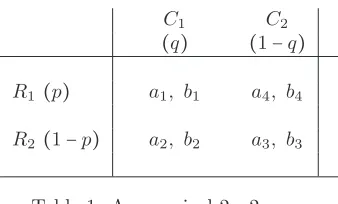
The game consists of a set of playersI= {R, C}, and two sets of actions for the two players: AR = {R1, R2} and AC = {C1, C2}. Outcomes, expressed in
utility units3
, are represented by the matrix shown in Table 1.
C1 C2
(q) (1−q)
R1 (p) a1, b1 a4, b4
[image:5.595.211.380.391.493.2]R2 (1−p) a2, b2 a3, b3
Table 1: A canonical 2×2 game
We define the mixed-strategy spaces ofR andC as follows:
∆(R) = {p∶AR→[0,1] ∣p(R1)+p(R2)=1}≡{(p,1−p) ∣p∈[0,1]},
∆(C)={q∶AC→[0,1] ∣q(C1)+q(C2)=1}≡{(q,1−q) ∣q∈[0,1]}.
The mixed strategy space is ∆=∆(R)×∆(C). Furthermore, since each player can choose only two possible actions, ∆(R) and ∆(C) can be identified with
[0,1]and ∆ can be identified with [0,1]2
.
Thepure-strategy best response correspondence ofR isBRR∶[0,1]→2AR,
whereBRR(q)is the set of actions of playerRwhich are best responses to the
mixed strategyq ofC.
Themixed-strategy best response correspondence ofR isψR∶[0,1]→2[0,1], being ψR(q) the set of mixed strategies of R which are best responses to the
mixed strategyq ofC. The same definitions hold for playerC.
3
Finally, we define the correspondence ψ ∶ [0,1]2
→ 2[0,1]
2
where ψ(p, q) =
ψR(q)×ψC(p). We recall that a NE is a mixed strategy profile (p, q)∈[0,1]
2
in which each player’s strategy is optimal for him, given the opponent strategy. Formally, if(p, q)∈[0,1]2
is a Nash equilibrium, thenp∈ψR(q)and q∈ψC(p)
i.e. (p, q) ∈ ψ(p, q) is a fixed point of the correspondence ψ. The logic is reversible, so(p, q)is a Nash equilibrium if and only if it is a fixed point of the correspondence ψ.
2.1
Utility function
In an expected utility framework, given a generic mixed strategy profile, the utility of player Rcan be expressed as in expression(1).
UR0(p, q)=a4p(1−q)+a3(1−p)(1−q)+a2q(1−p)+a1pq. (1)
In order to specify the utility function under CPT assumptions, we must analyse the ranking among outcomes. Suppose, for instance, that payoffs ai
satisfy the following ranking: a1>a2≥a3>a4≥0. We assume that outcomes
are already expressed in utility units. However, given the initial payoffs, an S-shaped value function – such that proposed in Tversky and Kahneman (1992) – and a reference point, we can always express original payoffs in utility units.
Using CPT the utility associated, for playerR, to a generic mixed strategy profile(p, q)is:
UR(p, q)=a4+(a3−a4)π(1−p+pq)+(a2−a3)π(q)+(a1−a2)π(pq). (2)
where π∶ [0; 1]→ [0; 1] is a weighting function, i.e. a function which mono-tonically distorts the probabilities. Trivially, whenπ(x)=x, we do not distort the probabilities. and (1) is the same of (2).Therefore, EUT is a special case of CPT.
2.2
Distorted probabilities
The idea of a weighting function for probabilities was formalized for the first time by Kahneman and Tversky (1979). It is a strictly increasing function
π∶[0; 1]→[0; 1]satisfying the conditionsπ(0)=0 andπ(1)=1. The weighting function proposed in Tversky and Kahneman (1992) is:
π(p)= p
γ
[pγ+(1−p)γ]γ1
. (3)
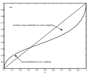
Tversky and Kahneman (1992) estimated γ = 0.61 for probabilities attached to gains and γ =0.69 for those attached to losses. Figure 1 shows the typical graph of expression (3). The inverse S-shape corresponds to the fact that people overweight very small probabilities and underweight average and large ones.
The complexity of this function determines some difficulties in the study of the sign of the derivative of the utility function4
. Indeed there is not a closed
4
The derivative of (3) with respect topis
π′
(p) =(γ−1)p
2γ−1
+ (p−p2
)γ−1
(p−pγ+γ)
[pγ+(1−p)γ]γ1+1
0 0.1 0.2 0.3 0.4 0.5 0.6 0.7 0.8 0.9 1 0
0.1 0.2 0.3 0.4 0.5 0.6 0.7 0.8 0.9 1
p
π(p)
[image:7.595.228.382.132.262.2]small probabilities are over−weighted moderate−large probabilities are under−weighted
Figure 1: CPT weighting function
form solution for the roots of its first derivative. To overcome this issue, we can specify a simpler version of the weighting function 3.
The reason to proceed in this way is simple. Our aim is to explore the be-havioural effects of introducing CPT in games, and analyse how this affects NE existence. Therefore, we can use a more manageable function which approxi-mates the original one (Expressed in 3). This approach gives us some results and insights on the effects on equilibria of CPT assumptions, which could ex-plain the differences between outcomes predicted by the theory and outcomes observed in reality.
2.3
A simple weighting function
The complexity of the probability weighting function (expression 3) leads to a major issue: it is not possible to derive a closed form solution for the maximi-sation problem. Therefore, we cannot give conditions for the existence of an equilibrium in the game.
However, we can define the following weighting function:
ω(p)={
√αp 0≤p≤α
1−√(1−α)(1−p) α≤p≤1 . (6)
forα∈(0,1), which is differentiable in(0,1).
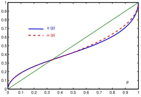
This function approximates the original Tversky and Kahneman (1992) Given a certain value of the parameterγ (for expression 3) we can find the parameterαwhich approximates this function. Moreover, our function hasαas fixed point (i.e. ω(α)=α), while for the KT weighting function withγ=.61, the fixed point isp≈1/3.Therefore, we can always find the parameter αwhich can approximate the function. In figure 2 we plot expression (6) withα=1/3 and expression (3) with γ=.61. As we can see, ω(p)seems to nicely approximate
π(p), provided that their fixed points are coincident.
The derivative of the utility functionUR(p, q)with respect topis
∂UR(p, q)
∂p =(a3−a4)π
′
(1−p+pq)(q−1)+(a1−a2)π
′
The aim of this paper is to investigate how the use of PT affects the equi-librium in a game. Since payoffs are expressed in utility units, the focus on the behavioural effect of distorted probability. Given that expression (3) is the most popular weighting function used in literature and given that expression (6) approximates nicely the original function, we beleive that our approach will preserve insights on the use of CPT in games.
0 0.1 0.2 0.3 0.4 0.5 0.6 0.7 0.8 0.9 1 0
0.1 0.2 0.3 0.4 0.5 0.6 0.7 0.8 0.9 1
π (p)
[image:8.595.225.369.215.314.2]p ω (p)
Figure 2: CPT weighting function
3
Nash Equilibria, best responses and CPT
In this section we will analyse some core results of applying CPT to a generic 2-player 2-strategy game, which can be represented in table 1.
In general we can express the problem as follows: given the sets of best responses for the two players GψR ={(p, q) ∣q∈[0,1], p∈ψR(q)} and GψC =
{(p, q) ∣p∈[0,1], q∈ψC(p)}. The intersection ofGψRandGψC determines the
set of NE. We can use this notation both under EUT and CPT.
The first case to be investigated is the presence either i) of a dominant strategy orii) of two indifferent strategies. In our setting – i.e. a 2–player 2– strategy game – we have at least one pure NE. In the most extreme case, when each player is inifferent between his two strategies, every combination (p, q)is a NE forp, q∈[0,1].
Proposition 1. Dominant Strategies. Dominant or indifferent strategies always emerge under Cumulative Prospect Theory, regardless to the weighting function used.
Proof. See Appendix 6
Our first result is that dominant strategies are preserved using CPT pref-erences. This result applies regardless to the type of weighting function used. Therefore, since EUT is a special case of CPT, the set of pure NE using EUT must coincide with the set of pure NE under CPT.
Corollary 2. When both players have a (strictly or weakly) dominant strategy, or two indifferent strategies, the set of pure Nash equilibria is the same both under EUT and CPT.
always a unique best response (or is indifferent between the two strategies). Thus, also using a structure of preferences which satisfies CPT, the best response set remains the same.
On the contrary, CPT may affects best responses when there is not a dom-inant strategy. We will analyse the special case in which payoff are such that:
a1 > a2 ≥ a3 > a4 ≥ 0, in order to provide an example of non existence of
equilibria. This is a direct result of the form of the weighting function and, consequently, of the utility function.
Proposition 3. Absence of dominant strategies. Using the weighting func-tion defined in Expression (6), and a1>a2≥a3>a4≥0, mixed equilibria may
not exist under CPT. When it exists, it can be shifted with respect to the EUT case.
Proposition 4. Using the weighting function defined in Expression (6), and
a1>a2≥a3>a4≥0, defining A= a1−a2
a3−a4, the condition A≥ 1−α
α is sufficient for
the continuity of the best response correspondence of player R.
Proof. See Appendix 6
Corollary 5. When Proposition 4 holds for both players, there will always exist at least one equilibrium. Thus this is a sufficient conditions for the existence of an equilibrium.
.
Introducing CPT in our framework has a dramatic effect. For certain values of the parameters – such thatA< 1−α
α – players find not optimal to mix between
their two pure strategies. Consequently, mixed equilibrium could not exist under CPT. This is the result of non–continuity of the best response function. On the other hand, whenA≥1−α
α , the optimal (mixed) strategy profile for each player
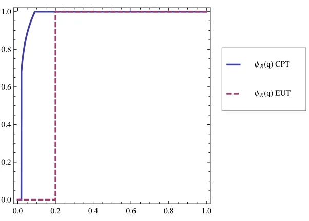
may be different with respect to the EUT case. When the equality holds the best response sets using the two approaches are the same (see Figure 5).
Moreover, when pure NE do not exist in the game, the above condition is a necessary condition for the existence of a mixed equilibrium.
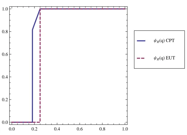
Figure 3 and 4 show the reaction curves using the two approaches (CPT and EUT). In our example, it is easy to see that with CPT preferences, playerR is willing to mix between his strategies although it would not be optimal under EUT.
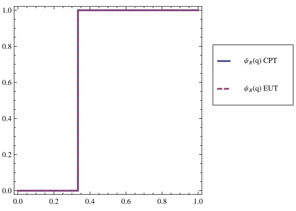
It is straightforward to see that if A = 1−α
α the reaction curves perfectly
coincide (Figure 5).
Consequently, even if a mixed equilibrium exist it could be different when assuming CPT; behavioural and experimental evidences may be explained by this assumption.
4
Results and comments
0.0 0.2 0.4 0.6 0.8 1.0 0.0
0.2 0.4 0.6 0.8 1.0
ΨRHqLEUT
[image:10.595.145.449.118.337.2]ΨRHqLCPT
Figure 3: Reaction curves with CPT and EUT witha1=6,a2=3,a3=2,a4=1,
α=1/3
This is a direct result of the special form assumed by the weighting function and, consequently, by players’ preferences. Indeed, we can explain this result under a more general framework.
The existence of a mixed equilibrium is subject to the condition that players will find optimal to mix between their available strategies. However, “non-expected utility maximizing players whose preferences cannot be represented by functions that are everywhere quasiconcave in the probabilities’ may be unwilling to randomize as equilibrium would require” (Crawford, 1990).
Continuity of reaction functions is a sufficient condition for the existence of a mixed equilibrium, Therefore. when Proposition 4 holds for both players there will always exist at least one equilibrium in the game. Given the structure of payoffs, the conditions imposed are based on the value of payoffs (i.e. the value ofA), and on the fixed point of the weighting function (α).
A characteristic of the CPT weighting function is that they are concave in a certain initial interval of probabilities – in our case between 0 andα– and then they are convex after the fixed point (see Figure 2).
First of all, we should notice that the expected utility under CPT (Expression n. 2) in the special case a1>a2 ≥a3 >a4≥0, results in a linear combination
of the probability weighting functions. Consequently, the form of the expected utility is a direct result of the form of the weighting function, since it is the linear combination of the weighting functions.
Therefore, we can address our result in a more general framework, in which the concavity – linearity, or convexity – of preferences affects the existence of mixed equilibria.
Secondly, the condition expressed in the proposition 4 may be interpreted as conditions for quasi–concavity or quasi–convexity, as we will see below.
0.0 0.2 0.4 0.6 0.8 1.0 0.0
0.2 0.4 0.6 0.8 1.0
ΨRHqLEUT
[image:11.595.147.448.121.337.2]ΨRHqLCPT
Figure 4: Reaction curves with CPT and EUT with a1 = 18, a2 = 8, a3 = 6,
a4=5,α=1/3
to mix between these two strategies – if the following condition is met:
a1q+a4(1−q)
´¹¹¹¹¹¹¹¹¹¹¹¹¹¹¹¹¹¹¹¹¹¹¹¹¹¹¹¹¹¹¹¹¹¹¹¹¹¹¸¹¹¹¹¹¹¹¹¹¹¹¹¹¹¹¹¹¹¹¹¹¹¹¹¹¹¹¹¹¹¹¹¹¹¹¹¹¹¶
R1
=a2q+a3(1−q)
´¹¹¹¹¹¹¹¹¹¹¹¹¹¹¹¹¹¹¹¹¹¹¹¹¹¹¹¹¹¹¹¹¹¹¹¹¹¹¸¹¹¹¹¹¹¹¹¹¹¹¹¹¹¹¹¹¹¹¹¹¹¹¹¹¹¹¹¹¹¹¹¹¹¹¹¹¹¶
R2
⇐⇒ A= a
1−a2
a3−a4
= 1−q
q (7)
Consequently,ifA>1−qq, he strictly prefersR1, and he prefersR2on the contrary.
Therefore, we can defineq∗ as the probabilityq which makes indifferentR, i.e. q∗ = 1
1+A. For smaller values ofq, strategyR1 is strictly preferred to R2,
and vice versa.
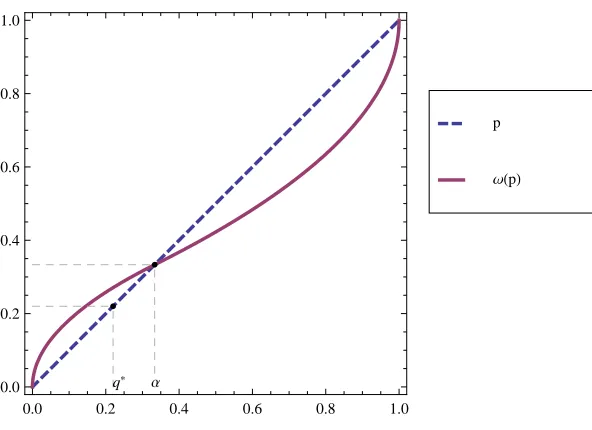
We find that a sufficient condition, under our special assumptions, for the existence of a mixed equilibrium is thatα≥ 1
1+A. Thus, we need the fixed point
of the weighting function to be greater or equal to the indifference probability using EUT, i.e. α≥q∗. This condition has a real neat graphic explanation (See Figure 6): the indifference point under EUT must lay in the quasi–concave part of the weighting function. When a1>a2≥a3>a4, the condition for concavity
of the weighting function are the same of the second order condition of the expected utility function.
This interpretation has three major consequences. On the one hand, we can link conditions for the equilibrium existence in a more general framework, which is the generic class of quasi–concave or quasi–convex preferences. Secondly, our results may be broaden considering other cases different froma1>a2≥a3>a4≥
0, now by looking at the whole expected utility function. Finally, we can use our insights for all types of weighting function, such as the original proposed by Tversky and Kahneman (1992) or that proposed by Prelec (1998).
For general cases, different froma1>a2≥a3>a4≥0, concavity is not
deter-mined by the condition α> 1
1+A . Although for the other cases it is difficult, if
0.0 0.2 0.4 0.6 0.8 1.0 0.0
0.2 0.4 0.6 0.8 1.0
ΨRHqLEUT
[image:12.595.146.448.122.337.2]ΨRHqLCPT
Figure 5: Reaction curves with CPT and EUT witha1=5,a2=3,a3=2,a4=1,
α=1/3
concavity/convexity of the expected utility function using numerical simulations (see for instance Figure 6).
5
An alternative approach
In the previous pages we mentioned that an alternative approach has been analysed by Metzger and Rieger (2009). In this section we will briefly explain the differences in the two papers, and the effect on the equilibrium properties of the models. Furthermore, we think that a very neat interpretation could be given to the two approaches.
In our paper we focus on the probability of a certain outcome, which is the result of two (mixed) strategies. This means that the probability of the event is distorted by players. By using this approach we follow the original idea of Kahneman and Tversky (1979), according to which “decision weights measure the impact of events on the desirability of prospects”.
On the other hand, Metzger and Rieger (2009)5
apply the following two step approach: first each player subjectively weights the probabilities (strategies) of her opponents, according to CPT; then she calculates her expectation, according to EUT.
This intermediate approach between CPT and EUT, is compatible with the Kakutani fixed point theorem (Kakutani, 1941; Nash, 1950, 1951) and, sub-stantially, it leads to a possible shift of the equilibrium points in the Nash Set. Thus the two authors find that a Nash equilibrium always exists in the game
5
0.0 0.2 0.4 0.6 0.8 1.0 0.0
0.2 0.4 0.6 0.8 1.0
ΩHpL
p
Α
[image:13.595.148.444.122.337.2]q*
Figure 6: CPT weighting function, and EUT indifference point
analysed.
In our opinion it is not possible to say what approach is preferable, since the two methods focus either on the probability of a single event which generates a certain utility, or on the probability of an opponent following a certain strategy. We, however, find some analogies to Crawford (1990).
In particular, we think that the alternative approach is linked to the def-inition of equilibrium in beliefs as defined by Crawford (1990), which requires
“each player’s beliefs about the other’s mixed strategy to be a (possibly degener-ate) probability distribution over the other’s best replies”.
This because Metzger and Rieger (2009) structure their analysis as follows. Given the probability distribution over the strategies of the opponent(s), the player would prefer a certain pure strategy. Then, he will mix among the pure strategies to maximise his payoff. Straigthforwadly, it is easy to see that this approach is compatible to Crawford (1990)6
.
We, however, need to do some remarks about this point. First of all, Craw-ford (1990) analyses the effect of applying a structure of preferences on monetary payoffs with mixed strategies. We, instead, refer to the way in which weight-ing functions are used in intermediate approach. Insights, however, remain the same, as well as for the interpretation of equilibrium.
Furthermore, our approach leads to some analytical difficulties which are not found in Metzger and Rieger (2009). Therefore, if on the one hand our approach is more consistent with the definition of Nash equilibrium, on the other hand, technical difficulties lead to less general results. Equilibrium always exist in Metzger and Rieger (2009), which is not our case. On the other hand, since we can consider the intermediate approach as an equilibrium in beliefs, we should
6
notice that “the predictive content of an equilibrium is small: it predicts only that each player uses an action that is a best response to the equilibrium beliefs”
(Osborne and Rubinstein, 1994).
6
Conclusions
We investigated how the use of CPT affect a 2x2 non-cooperative game. The first result was that all the pure strategy Nash equilibria predicted in the EUT framework are preserved. We however find that the set of mixed equilibria could be either empty or different from the one under EUT assumption. In only one case the two approaches lead to the same set of equilibria.
Due to analytical difficulties we are able to study only a case where payoffs have some restrictions. However, we can interpret the conditions for existence of NE as conditions for quasi-concavity of the expected utility function. In this way we can generalise to all form of weighting functions and to a more general structure of payoffs, so to make wider, and more consistent to the previous literature, our results.
References
Abdellaoui, M. (2000). Parameter-free elicitation of utility and probability weighting functions. Management Science,46(11), 1497–1512.
Abdellaoui, M., Vossmann, F., and Weber, M. (2003). Choice-based elicitation and decomposition of decision weights for gains and losses under uncertainty. InCentre for Economic Policy Research Discussion Paper 3756.
Allais, M. (1953). Le comportement de l’homme rationnel devant le risque: Critique des postulats et axiomes de l’´ecole Am´ericaine.Econometrica,21(4), 503–546.
Barberis, N., Huang, M., and Santos, T. (2001). Prospect Theory and Asset Prices. Quarterly Journal of Economics,116(1), 1–53.
Benartzi, S. and Thaler, R. (1995). Myopic loss aversion and the equity premium puzzle. The Quarterly Journal of Economics, 110(1), 73–92.
Bleichrodt, H. and Pinto, J. (2000). A parameter-free elicitation of the proba-bility weighting function in medical decision analysis. Management Science, 46(11), 1485–1496.
Camerer, C. (1995). Individual Decision Making. InHandobook of Experimental Economics, pages 587–703. Princeton University Press.
Camerer, C. (2000). Prospect theory in the wild: Evidence from the field.
Advances in Behavioral Economics.
Camerer, C. F. and Ho, T.-H. (1994). Violations of the betweenness axiom and nonlinearity in probability. Journal of Risk and Uncertainty,8, 167–196.
Crawford, V. P. (1990). Equilibrium without independence. Journal of Eco-nomic Theory,50(1), 127 – 154.
Dekel, E., Safra, Z., and Segal, U. (1991). Existence and dynamic consistency of nash equilibrium with non-expected utility preferences. Journal of Economic Theory,55(2), 229 – 246.
Gilboa, I. (1987). Expected utility with purely subjective non-additive proba-bilities. Journal of Mathematical Economics,16(1), 65–88.
Jolls, C., Sunstein, C., and Thaler, R. (1998). A behavioral approach to law and economics. Stanford Law Review,50(5), 1471–1550.
Kahneman, D. and Tversky, A. (1979). Prospect theory: An analysis of decision under risk. Econometrica: Journal of the Econometric Society, 47(2), 263– 291.
Kakutani, S. (1941). A generalization of brouwer’s fixed point theorem. Duke Mathematical Journal,8(3), 457–459.
Markowitz, H. (1952). The utility of wealth. Journal of Political Economy, 60(2), 151–158.
McNeil, B., Pauker, S., Sox Jr, H., and Tversky, A. (1982). On the elicitation of preferences for alternative therapies. New England journal of medicine, 306(21), 1259–1262.
Metzger, L. and Rieger, M. (2009). Equilibria in games with prospect theory preferences. Working Paper.
Nash, J. (1950). Equilibrium points in n-person games. Proceedings of the National Academy of Sciences of the United States of America,36(1), 48–49.
Nash, J. (1951). Non-cooperative games. The Annals of Mathematics, 54(2), 286–295.
Osborne, M. and Rubinstein, A. (1994). A course in game theory. The MIT press.
Prelec, D. (1998). The probability weighting function. Econometrica, pages 497–527.
Quattrone, G. and Tversky, A. (1988). Contrasting rational and psychological analyses of political choice. The American political science review, 82(3), 719–736.
Quiggin, J. (1982). A theory of anticipated utility. Journal of Economic Behav-ior & Organization,3(4), 323–343.
Schmeidler, D. (1986). Integral representation without additivity. Proceedings of the American Mathematical Society, 97(2), 255–261.
Schoemaker, P. J. H. (1982). The expected utility model: Its variants, purposes, evidence and limitations.Journal of Economic Literature,20(2), pp. 529–563.
Starmer, C. (2000). Developments in non-expected utility theory: The hunt for a descriptive theory of choice under risk. Journal of Economic Literature, 38(2), pp. 332–382.
Tversky, A. and Fox, C. (1995). Weighing risk and uncertainty. Psychological review,102(2), 269–283.
Tversky, A. and Kahneman, D. (1992). Advances in prospect theory: Cumu-lative representation of uncertainty. Journal of Risk and uncertainty, 5(4), 297–323.
Von Neumann, J. and Morgenstern, O. (1944). Theory of games and economic behavior. Princeton University Press.
Wu, G. and Gonzalez, R. (1996). Curvature of the probability weighting func-tion. Management Science, 42(12), 1676–1690.
Appendix
Proof of Proposition 1
In our setting (Table 1) pure NE arise when both players either have a dominant strategy or are indifferent between their strategies. Therefore we need to prove that using CPT these strategies remain best response for a generic player. We will consider three cases: (1)R[C] has a strictly dominant strategy, for instance
R1 [C1]; (2) R[C] has a weakly dominant strategy; and (3) the two strategies
R1[C1] andR2 [C2] are indifferent. We will consider only one player, since the
same logic applies for both players.
Let’s consider the last and simplest case. Indifference between the two strate-gies arises when each strategy leads to the same payoffs, i.e. a1=a2≥a3=a4.
In this case,R′s expectation using CPT is
UR(p, q)=⎧⎪⎪⎪⎨⎪⎪⎪
⎩
a3+(a1−a3)π+(q) a1≥a3≥0
a1π+(q)+a3π−(1−q) a1>0>a3
a1+(a3−a1)π−(1−q) 0≥a1≥a3
. (8)
WhileR′s expectation using EUT is:
U0
R(p, q)=a1q+a3(1−q). (9)
Note that Expressions (8) and (9) are independent of p. Therefore, the set of best responses, both under EUT and CPT, isψR(q)=[0,1]∀q∈[0,1].
Now suppose thatR1 weakly dominates R2. Without loss of generality we
assume thata1>a2≥a3=a4 (Table 1).
PlayerR′s expectation using CPT is
UR(p, q)=
⎧⎪⎪⎪⎪ ⎪⎨ ⎪⎪⎪⎪⎪ ⎩
a3+(a2−a3)π+(q)+(a1−a2)π+(pq) a1>a2≥a3≥0
a3π−(1−q)+a2π+(q)+(a1−a2)π+(pq) a1>a2≥0>a3
a2π−(1−pq)+(a3−a2)π−(q)+a1π+(pq) a1≥0>a2≥a3
a1+(a2−a1)π−(1−pq)+(a3−a2)π−(1−q) 0>a1>a2≥a3
.
R′s expectation using EUT is showed as follows:
UR0(p, q)=a3+(a2−a3)q+(a1−a2)pq. (11)
Equations (10) and (11) show that expectation ofR is independent onpwhen
q=0 and thenψR(0)=[0,1]. For q≠0 Since (1)pq andπ+(pq)are increasing
in p, and (2) π−(1−qp) is decreasing in p, the expected utility is maximized
choosingp=1 for all q≠0 , i.eψR(q)={1}∀q∈]0,1]. As in the previous case,
the best response set is equal under EUT and CPT.
Finally, assumeR1strictly dominatesR2, i.e. a1≥a4>a3≥a2. In this case,
using EUT as well as using CPT, expected utility is maximized by p=1 for all
q, i.eψR(q)={1}∀q∈[0,1].
Proof of proposition 3
Sincea1>a2≥a3>a4, consequently,R’s expected utility for a generic strategy
profile(p, q)is:
UR(p, q)=a4+(a3−a4)π(1−p+pq)+(a2−a3)π(q)+(a1−a2)π(pq), (12)
whose derivative with respect topis
∂UR(p, q)
∂p =(a3−a4)π
′(
1−p+pq)(q−1)+(a1−a2)π′(pq)q. (13)
We can study the sign of this derivative, which is
∂UR(p, q)
∂p >[<;=]0 ⇔ A=
a1−a2
a3−a4
>[<;=]1−q
q ⋅
π′(pq+1−p)
π′(pq) . (14)
Note that we are using the weighting function defined in Expression (6), whose derivative is:
ω′(p)=⎧⎪⎪⎪⎨⎪⎪⎪
⎩
1 2
√α
p 0<p≤α
1 2
√
(1−α)
(1−p) α≤p<1
. (15)
Sincepq+1−p≥pq, and using Expression (15), we can distinguish three cases:
1. In the first case we have
α≥pq+1−p≥pq ⇔ p≥1−α
1−q,
and Expression (14) becomes:
A> 1−q
q
√
pq
pq+1−p ⇔ p<
A2
q
(1−q)(1−q+A2q) =C(q). (16)
2. The second instance arises if
pq+1−p≥pq≥α ⇔ p≥ α
q,
then Expression (14) becomes:
A>1−q
q
√
1−pq
p−pq ⇔ p>
1−q
0 0.1 0.2 0.3 0.4 0.5 0.6 0.7 0.8 0.9 1 0
0.2 0.4 0.6 0.8 1
q
ψR
(q)
ψR(q)
ψR(q)
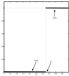
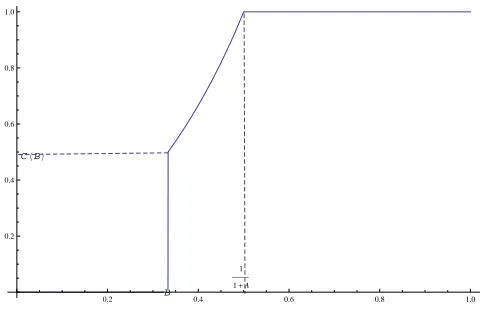
[image:18.595.136.250.134.259.2]A*
Figure 7: R best response correspondence whenA< 1−α α .
3. Finally, if
pq+1−p>α>pq ⇔ p<min{α
q,
1−α 1−q},
expression (14) becomes:
A>
√
1−α
α
1−q
q ⇔ q>
1−α
(1−α+A2α)=B. (18)
Note that in expressions (16), (17) and (18) we have defined the quantities
C(q)andD(q)(depending onq) andB (not depending onq).
Under our hypotheses, we have only two parameters. These are two between
A,αandB. Thus we discuss the general case, distinguishing the following three cases.
Case I A<1−α
α ⇔ α<
1
1+A ⇔ B>α,
Case II A>1−α
α ⇔ α>
1
1+A ⇔ B<α,
Case III A=1−α
α ⇔ α=
1
1+A ⇔ B=α.
Case I,A< 1−α
α . PlayerC chooses his strategy in the interval[0,1], which
can be partitioned by:
0<α< 1
1+A <B<1.
If 0≤q≤α, thenpq ≤q≤α. If pq+1−p≥α, i.e. p∈[0,1−α/1−q], thus
U′<0 iffA<√1−α
α
1−q
q i.e. iffq<B which is true beingq≤α<B.
If p∈]1−α/1−q,1], thus U′<0 iffp>C(q), that is true if C(q)≤1−α/1−q which is equivalent toq<B, that is true. Thus if 0≤q≤α, then U′(p)<0 for allp∈[0,1].
If 1≥q>B>α, thuspq+1−p>α. Ifpq≤α, i.e. p∈[0, α/q]then U′>0 iff
A>√1−α
α
1−q
q , i.e. iffq>B that is true. Ifp∈]α/q,1],U
B CHBL
1 1+A
0.2 0.4 0.6 0.8 1.0
[image:19.595.125.367.124.281.2]0.2 0.4 0.6 0.8 1.0
Figure 8: R best response correspondence
is true if α/q≥D(q)i.e. q>B that is true. Thus if 1≥q>B>α,U′(p)>0 for allp∈[0,1].
Ifα<q<B, then pq+1−p>α. If pq≤α, i.e. p∈[0, α/q]then U′<0 iff
A<√1−α
α
1−q
q i.e. iffq<B that is true. If p∈]α/q,1], U
′<0 iffp<D(q). The
position ofD(q)in the interval[0,1]depends on the confront ofqand 1/(1+A). If q∈]α,1/(1+A)] thenD(q)≥1 and sop<D(q)is true, i.e U′(p)<0 for all
p ∈ [0,1]. If q ∈]1/(1+A)/B[ then U′(p) < 0 if p < D(q) and U′(p) > 0 if
p>D(q).
In Case I, we conclude in any case that for allq∈[0,1],ψp(q)⊆{0,1}. Now
the question regards the confront between U(0)andU(1). SinceU(0)>U(1) when q < π−1
( 1
1+A) =A, then the graph ofψq(p) is that showed in figure 8,
where q1/2 = A. Let us note how this is the case where equilibria could not
exist.
Case II,A>1−α
α . In this case the interval[0,1]can be partitioned by
0<B< 1
1+A<α<1.
If 0≤q≤B<α, thenpq≤q<α. Ifpq+1−p≥α, i.e. p∈[0,1−α/1−q], thus
U′≤0 iffA≥√1−α α
1−q
q i.e. iffq≤B which is true.
If p∈]1−α/1−q,1], thus U′≤0 iffp≥C(q), that is true if C(q)≤1−α/1−q which is equivalent to q≤B, that is true. Thus if 0≤q≤B<α, then U′(p)≤0 for allp∈[0,1].
Ifα≤q≤1, thus pq+1−p≥α. If pq ≤α, i.e. p∈[0, α/q]then U′≥ 0 iff
A≥√1−α
α
1−q
q , i.e. iffq≥B that is true. Ifp∈]α/q,1],U
′≥0 iffp>D(q), that
is true ifα/q≥D(q)i.e. q≥B that is true. Thus ifα≤q≤1, thenU′(p)≥0 for
allp∈[0,1].
IfB≤q≤α, thenpq≤q≤α. If pq+1−p≥α, i.e. p∈[0,1−α/1−q], thus
U′≥0 iffA≥√1−α α
1−q
q i.e. iffq≥B which is true.
we have that
1−α 1−q ≤↑
q≥B
C(q) ≤
↑
q≤ 1 1+A
1
Thus, ifq∈[1/1+A, α], C≥1≥pand then U′(p)≥0. At this point, regarding the sign of the derivative U′(p)we have the following result. Ifq∈[0, B]then
U′(p)≤0 for allp∈[0,1]and ifq∈[1/(1
+A),1]thenU′(p)≥0 for allp∈[0,1]. If B < q ≤ 1
1+A, thus the sign of the derivative U
′(p) changing p is the
following: If p∈[0, C(q)[ thenU′(p)>0, while ifp∈]C(q),1]then U′(p)<0. Being U(p)continuous in C(q)this means that in this case the best response correspondence of R is just ψR(q)= {C}. The quantity C = A
2
q
(1−q)(1−q+A2q) is
increasing inq, sinceC′(q)≥0. Thus, whenqmoves fromBto 1/(1+A),C(q) increases fromC(B)=1/C(α)toC(1/1+A)=1.
Finally the graph ofψR(q)is that showed in figure 8. We have just to justify
the shape ofψR(B)=[0, C(B)].
Ifq=B<α, then
1−α
1−q =C(B)= 1
C(α).
Ifp∈[0, C(B)]then
U′(p)=A−1−B
B
√
1−α
α B
1−B =a−A=0.
Ifp∈]C(B),1],
U′(p)=A−
√
pB
pB+1−p,
that is negative ifp>[C(α)]−1=C(B). From the sign ofU′(p)we elicit that, forq=B,U(p)is constant ifp∈[0, C(B)]and decreasing ifp∈]C(B),1]. Thus
ψR(B)=[0, C(B)].
Let us note that in this Case II we have the continuity of the best response correspondence of player R. This condition, together with the continuity of the best response of the other player ensures the existence of an equilibrium. However this equilibrium could be shifted with respect to prediction of EUT.
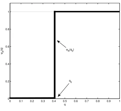
Case III, A= 1−α
α . This hypothesis is equivalent to say that (a1−a2)α=
(a3−a4) (1−α). Note that 1/(1+A)=αandπ− 1
(1/1+A)=π−1(α)=α. Since
αp≤αand αp+1−p≥α, thus the utility
UR(p, α)=a4+(a3−a4)+(a2−a3)π(α)+√p[α(a1−a2)−(1−α) (a3−a4)]=
=a4+(a3−a4)+(a2−a3)π(α)
does not depend onpand then, ψR(α)=[0,1]. Finally the graph of ψR(q)is
showed in figure 9, with q0= α. Thus, in Case III, CPT prediction coincides
0 0.1 0.2 0.3 0.4 0.5 0.6 0.7 0.8 0.9 1 0
0.2 0.4 0.6 0.8 1
q ψR
(q)
[image:21.595.139.345.322.510.2]q0 ψR(q0)