A multiphase model for tissue construct growth in a perfusion bioreactor

A multiphase model for tissue construct growth in a

perfusion bioreactor

R. D. O’Dea, S. L. Waters

_{& H. M. Byrne}

School of Mathematical Sciences, University of Nottingham

University Park, Nottingham, NG7 2RD

†

_{Mathematical Institute, 24-29 St Giles’, Oxford, OX1 3LB}

Abstract

The growth of a cell population within a rigid porous scaffold in a perfusion bioreactor is studied, using a three phase continuum model of the type presented by Lemon et al. (2006) to represent the cell population (and attendant extracellular ma-trix), culture medium and porous scaffold. The bioreactor system is modelled as a two-dimensional channel containing the cell-seeded rigid porous scaffold (tissue con-struct) which is perfused with culture medium. The study concentrates on (i) cell-cell and cell-scaffold interactions and, (ii) the impact of mechanotransduction mechanisms on construct composition.

A numerical and analytical analysis of the model equations is presented and, de-pending upon the relative importance of cell aggregation and repulsion, markedly dif-ferent cell movement is revealed. Additionally, mechanotransduction effects due to cell density, pressure and shear stress-mediated tissue growth are shown to generate qualitative differences in the composition of the resulting construct. The results of our simulations indicate that this model formulation (in conjunction with appropriate experimental data) has the potential to provide a means of identifying the dominant regulatory stimuli in a cell population.

1

Introduction

networks to tissue-level patterning and mechanics (Peirce et al., 2006). Due to their im-portance in (for instance) tissue engineering, and various pathological conditions, tissue growth processes have inspired a huge range of theoretical and experimental studies (see Araujo & McElwain (2004), Cowin (2000, 2004), Curtis & Riehle (2001) and Sipe (2002) for reviews).

In vitro tissue engineering, which involves creating replacement tissue in the

labora-tory from a sample of healthy cells or small explants, has the potential to alleviate the chronic shortage of tissue available from donors (Curtis & Riehle, 2001). Static culture for cell monolayer and small explants has been employed in vitro for many years; however, limitations in the diffusion of nutrients and waste products mean that scale-up to produce constructs of a size appropriate for implant results in the formation of constructs with a vi-able, proliferating periphery but a necrotic core (Cartmell & El Haj, 2005). To rectify this, bioreactors, which enable control of the culture environment via circulation/mixing strate-gies and provision of growth factors and other cell-signalling molecules, are widely used. As well as improving mass transfer, such strategies have a profound effect on the cells’ mechanical environment, the consequences of which will be specific to the cell population in question. For instance, fluid flow can have deleterious effects on cartilage regeneration; in contrast, many studies have shown that stimulation via fluid shear stress enhances bone tissue formation (Bakker et al., 2004; Han et al., 2004; Klein-Nulend et al., 1998, 1995b; Weinbaum et al., 1994; You et al., 2000, 2001). Many bioreactors are therefore designed specifically to provide appropriate mechanical stimulation to cell cultures via, e.g. fluid shear stress, or tensile or compressive forces applied on the macroscale or via magnetic particles embedded in the cell membrane (see Cartmell & El Haj (2005) and Martin et al. (2004) for a review). These stimuli are integrated into the cellular response via a process known as mechanotransduction.

Much research has been concentrated on the study of cartilage and bone tissue regen-eration, motivated by the notorious incapacity of the former to self-repair (Lemon & King, 2007) and the response of the latter to its mechanical environment; an experimental study of bone cell response to mechanical loading provided the inspiration for this research. Advances in the understanding of the mechanisms that regulate tissue growth via experi-mental or theoretical studies promise to improve the integrity and viability of the resulting tissue constructs; idealised theoretical studies aim to predict optimal protocols for tissue growth, suggest explanations for observed tissue growth phenomena and can provide in-sights useful in the design of bespoke bioreactor systems.

level include Jaecques et al. (2004), McGarry et al. (2004) and Tracqui & Ohayon (2004). The effect of growth-induced (residual) stresses on tissue growth within a macroscale mul-tiphase framework was investigated by Roose et al. (2003), employing a poroelastic model to determine the stress within, and surrounding, a tumour spheroid. Araujo & McElwain (2005) also presented a general multiphase framework suitable for the consideration of such stresses. Employing a two-phase model, Byrne & Preziosi (2003a) considered the in-fluence of the cells’ environment on their proliferative rate in the context of tumour growth. The tumour was modelled as a viscous fluid phase interacting with an inviscid extracellular fluid. The proliferation of tumour cells was dependent upon nutrient availability (governed by an advection-diffusion equation) and cell density, and a step function was used to switch between two different density and nutrient-dependent responses as the nutrient availability crosses a threshold value. By introducing a parameter associated with the cell’s response to growth-induced stress, a critical stress level was predicted, above which the tumour is eliminated. Chaplain et al. (2006) presented a similar model considering tumour cells, normal cells, their associated extracellular matrices (ECM) and a matrix-degrading en-zyme. A mollified step function was used to model the transition between the proliferative response of the cells in response to stress. It was shown that reduced contact inhibition or sensitivity to the compressive stress (modelled as proportional to the total tissue volume fraction) leads to elevated proliferation of the tumour cells.

considered and differences between the predicted tissue composition in each case illus-trated the potential use of the model to predict the dominant regulatory stimuli in a cell population.

Studies which consider specifically tissue growth in porous scaffolds include Malda

et al. (2004) in which the development of oxygen gradients in the absence of perfusion

was investigated using a simple diffusion-consumption model. Parameter estimation was achieved via comparison with experimental data. Three-dimensional fluid flow through porous scaffolds in a perfusion bioreactor was studied by Porter et al. (2005) in which a detailed model of a porous scaffold was obtained via micro-computed tomography imag-ing and the flow profile calculated usimag-ing the Lattice-Boltzmann method. Relatimag-ing simula-tion results to experimental results, it was concluded that a mean pore-surface shear stress of5×10−5_{Pa corresponds to increased cell proliferation and viability. Raimondi (2004)}

demonstrated that the material properties and cell viability of constructs resulting from per-fusion show a two-fold improvement compared to static culture; computational modelling was used to quantify the fluid-dynamical environment at the microscopic level. Modelling of both cell growth and fluid flow within a three-dimensional scaffold in a perfusion biore-actor was considered by Coletti et al. (2006). The flow through the scaffold was governed by Brinkman’s equation and nutrient distribution was described by a reaction-advection-diffusion equation. Cell growth was assumed to depend upon local nutrient availability via an ordinary differential equation.

studies, we represent the cells and associated ECM as a viscous fluid phase that is distinct from the culture medium; the porous scaffold is modelled as a rigid porous medium. The applicability of the model is therefore restricted to tissue constructs whose solid character-istics are dominated by scaffold rigidity. We remark, however, that our generic modelling framework is versatile allowing, for example, elastic or viscoelastic constitutive modelling assumptions for the cell or scaffold phases. Since the cells and ECM are modelled as a sin-gle phase, the interactions between the cells and the ECM are nesin-glected; furthermore, the replacement of degrading scaffold by proteoglycan and collagen deposition (for example) is not considered.

We investigate two factors which are of key importance in the growth and adaptation of engineered tissue constructs: (i) cell-cell and cell-scaffold interactions and, (ii) the impact of mechanotransduction mechanisms on construct morphology (specifically, we consider density, pressure and shear stress-mediated tissue growth). As noted above, despite many tissues sharing common mechanotransduction pathways, the influence of the mechanical environment will be specific to the cell population in question. In this paper, we employ our generic modelling framework to investigate a range of biologically-inspired mechan-otransduction mechanisms and, in so doing, demonstrate the importance of such effects to in vitro tissue growth and the ability of our model to accommodate a wide variety of such considerations. Conclusions relevant to specific tissue engineering systems may in principle be obtained by modifying the mechanotransduction response functions in line with appropriate experimental data; however, such modifications are beyond the scope of this paper. The influence of perfusion on construct growth is demonstrated by comparing the construct composition resulting from static and perfusive culture conditions. Nutrient-limited growth is not considered here so that we may focus on mechanotransduction. We demonstrate that the relaxation of the large drag assumption and consideration of cell-cell and cell-cell-scaffold interactions result in starkly different cell-cell behaviour to that found in O’Dea et al. (2008).

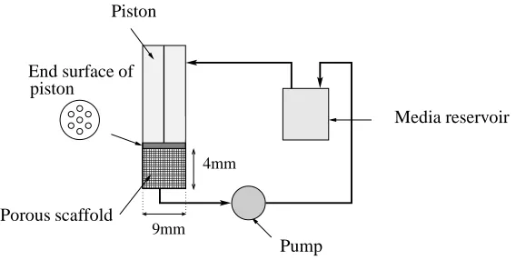
The perfusion bioreactor under consideration is based upon that employed by El-Haj

et al. (1990) which comprises a tissue construct within a culture medium-filled cylinder

forcing provided by the piston.

PLLA scaffold

00000 00000 00000 00000 00000 00000

11111 11111 11111 11111 11111 11111

9mm End surface of piston

Porous scaffold

Media reservoir

Pump Piston

4mm

9mm

Figure 1: The bioreactor system of El-Haj et al. (1990).

The structure of this paper is as follows. In§2 we present the three-phase governing equations; employing the long-wavelength limit (assuming that the bioreactor is long and thin) and considering constant, spatially-homogeneous scaffold porosity, we reduce the system to a pair of differential equations governing the cell phase volume fraction and the culture medium pressure, together with appropriate boundary conditions. Solutions to these equations are presented in§§3 and 4.

In§3, uniform growth is considered; numerical simulations are presented in§3.1 and validated against analytic solutions in the limit for which the cell volume fraction is asymp-totically small (§3.2). In§3.3, the influence of cell-cell and cell-scaffold interactions on tissue growth is investigated further by considering simplified functional forms for these effects. Lastly, in§4, we consider mechanotransduction-affected growth, studying the re-sponse of a cell population to the local density, pressure and shear stress. A discussion of the model results and their applications within the field of tissue engineering is given in

§5, together with suggestions for further work.

2

A three phase model for tissue construct growth

We consider the growth of a tissue construct within a nutrient-rich fluid culture medium and investigate the effect of cell-cell and cell-scaffold interactions, as well as that of mechanotransduction, on the growth of a tissue construct within a perfusion bioreactor. The bioreactor under consideration is based upon a system employed by El-Haj et al. (1990) (see§1) which we represent as a two-dimensional channel containing a mixture of interacting phases. A two-dimensional channel geometry is employed for simplicity; how-ever, generalisation to a cylindrical geometry is straightforward. The multiphase mixture comprises two viscous fluids and one rigid, porous phase. The cells and ECM, which are represented by a single phase (henceforth denoted the “cell phase”), and culture medium are modelled as viscous fluids, and the remaining rigid phase represents the scaffold. Tis-sue growth is represented by an increase in cell phase volume fraction, corresponding to the combined effects of cell proliferation and ECM deposition. Viscous fluid-based mod-els for biological tissue growth have been widely used (see e.g. Byrne et al. (2003), Byrne & Preziosi (2003b), Franks (2002) and Franks & King (2003)); such models are appropri-ate when the timescale of elastic relaxation is short in comparison to that of growth (Bittig

et al., 2008; Franks & King, 2003; King & Franks, 2004). Perfusion is represented by a

pressure-driven flow of culture medium.

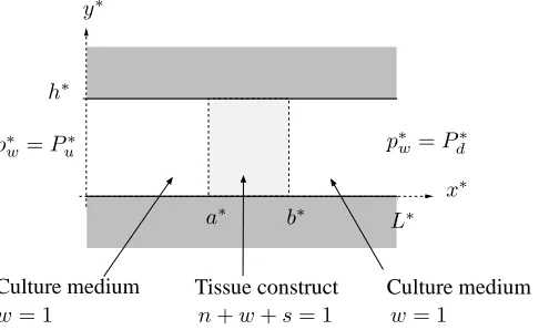
Tissue construct

Culture medium Culture medium

w= 1 n+w+s= 1 w= 1

x∗

y∗

h∗

L∗

a∗ _b∗

p∗

w=Pu∗ p

∗

w=Pd∗

Figure 2: Definition sketch: a two-dimensional channel of lengthL∗ _{and widthh}∗

con-taining a construct of lengthb∗_−a∗_.

A Cartesian coordinate systemx∗ = (x∗, y∗)is chosen with corresponding coordi-nate directions (xˆ,y) and the channel occupiesˆ 0 6 x∗ 6 L∗, 0 6 y∗ 6 h∗. In this

paper, asterisks distinguish dimensional quantities from their dimensionless equivalents. We associate with the cell, culture medium and scaffold phases a volume fraction denoted,

tensorσi (wherei = n, w, sdenotes variables associated with each phase) and assume

that these are functions ofx∗andt∗, wheret∗represents time.

For convenience, we confine the tissue construct to the regiona∗_6x∗_6b∗_{in which}

s >0(see figure 2), stipulating that the cell phase must remain confined within the

scaf-fold. We achieve this by imposing a no-flux boundary condition on the cell phase at the scaffold edge. Formulating the problem in this way allows us to simplify the governing equations in the up- and downstream regions, whilst retaining the full complexity of the three phase system within the construct region. The problem may be solved separately in each region, and the solutions coupled together via appropriate conditions.

The multiphase model takes the form of mass and momentum balances for each phase, together with appropriate constitutive laws. Neglecting inertial effects and assuming that each phase is incompressible with the same density, the equations governing theith_phase

(with volume fractionφi) are as follows (see Lemon et al. (2006)):

conservation of mass: ∂φi

∂t∗ +∇

∗_·(φ

iu∗_i) =S_i∗+D∗∇∗2φi; (2.1)

conservation of momentum: ∇∗·(φiσ∗_i) +

X

j6=i

F∗

ij =0, (2.2)

in whichS∗

i is the net material production term associated with phasei; so that mass is

conserved, we assumePS∗

i = 0. F∗ij is the force exerted by phasejon phaseiwhich

obeysF∗

ij =−F∗ji. Conservation conditions may be obtained by summing equations (2.1)

and (2.2) over all phases and exploiting the no-voids condition:Pφi= 1.

We remark that a diffusive term has been added to the mass conservation equation (2.1) and for simplicity the diffusivity of each phase is assumed to be equal; whilst cells do exhibit random motion, in this model the growth and flow-driven velocity field is the dominant mechanism giving rise to cell movement and diffusive terms are expected to be negligible (Franks et al., 2003; King & Franks, 2004). However, we retain these terms for numerical convenience since they eliminate the moving boundaries between the tissue construct and culture medium, ensuring that we need not track explicitly the sharp interface which is evident whenD∗_{= 0.}

stan-dard viscous stress tensors for these phases (with dynamic and bulk viscositiesµ∗

i, λ∗i;

i=n, w). For consistency, we choose the same form forσs, taking the limitµ∗s → ∞,

us→0.

The interphase forcesF∗

ijcomprise contributions from interphase viscous drag (which

is assumed to be proportional to the volume fraction of each phase and their relative ve-locity) and active forces arising between the phases. We assume that the cell phase gen-erates an intraphase pressure,Σ∗

n, resulting from interactions within the cell phase such

as osmotic stresses or surface tension within cell membranes. Additionally, tractions be-tween the cell and scaffold phases give rise to an additional pressure contribution,ψ∗

ns

(see Lemon et al. (2006) for more details). Assuming that interactions between the culture medium and scaffold phases are limited to viscous drag we find that the pressure in the cell phase is related to that in the culture medium via:

p∗n =p∗w+ Σn∗+ (1−θ)ψns∗ , (2.3)

and the interphase forces are given by:

F∗

nw=θp∗w∇∗n+k∗nw(u∗w−u∗n) =−F∗wn, (2.4)

F∗

sw =p∗w(1−θ)∇∗n+k∗(θ−n)(1−θ)u∗w=−F∗ws, (2.5)

F∗

ns= (p∗w+ψns∗ ) (1−θ)∇∗n−k∗n(1−θ)u∗n=−F∗sn, (2.6)

wherek∗_{is the coefficient of viscous drag which is assumed to be constant. The interphase}

interaction termsΣ∗

nandψns∗ and the material production rates (accommodating a range of

tissue growth processes) will be specified once the model has been cast in dimensionless form.

We non-dimensionalise as follows:

x∗=L∗x, t∗=t/K_m∗, u∗_i =K_m∗L∗ui, Si∗=Km∗Si,

(p∗

i,Σ∗n, ψns∗ ) =Km∗µ∗w(pi,Σn, ψns)

)

(2.7)

whereK∗

m is a typical tissue growth rate and the channel now occupies0 6 x 6 1,

06y6h=h∗_/L∗_{; the length of the construct isa6x6b, where(a, b) = (a}∗_{, b}∗_)/L∗_.

A viscous scaling is employed for the pressure in each phase (p∗

i) since we assume that

to be ofO(1)both in static (in which the flow is a consequence of tissue growth only) and perfusive culture conditions, employing fast growth rates to minimise computation time and to illustrate features of the system.

In dimensionless form, the model equations are:

∂n

∂t +∇ ·(nun) =Sn+D∇

2_{n, (2.8)}

∇ ·(nun+ (θ−n)uw) = 0; (2.9)

(θ−n)∇pw+kn(θ−n)(uw−un) +k(1−θ)(θ−n)uw−

∇ ·(θ−n)(∇uw+∇uTw) +γw(θ−n)∇ ·uwI = 0, (2.10)

∇ ·−(θpw+nΣn+n(1−θ)ψns)I+µnn(∇un+∇uT_n) +

γnn∇ ·unI+ (θ−n)(∇uw+∇uT_w) +γw(θ−n)∇ ·uwI+

∇n(1−θ)ψns−kn(1−θ)un−k(θ−n)(1−θ)uw=0.(2.11)

Equations (2.8) and (2.9) are statements of conservation of mass for the cell phase and the multiphase mixture; equation (2.10) expresses conservation of momentum for the culture medium and (2.11) is the momentum equation for the two phase mixture of cells and culture medium. We employ this equation in preference to the momentum equation for the three phase mixture for convenience (see Lemon & King (2007)). Assuming that the scaffold porosity is constant in space and time enabled significant simplification of the three-phase governing equations, the rigid scaffold phase only appearing via the constant porosity,θ, and the cell-scaffold interactions.

The dimensionless parametersD,µn,k,γwandγnare defined:

D= D

∗

K∗

mL∗

, µn= µ

∗

n

µ∗

w

, k= k

∗_L∗2

µ∗

w

, γw= λ

∗

w

µ∗

w

, γn = λ

∗

n

µ∗

w

. (2.12)

The physical interpretation of the dimensionless diffusion coefficient (or inverse Peclet number)D, relative viscosity µn, and drag coefficientkis self-evident. The parameter

γidescribes the relative importance of the viscosity associated with the rate of change of

volume of theith_{phase compared to that associated with fluid shear. It is usual to take}

λ∗

i =−2µ∗i/3implyingγw=−2/3andγn =−2µ∗n/3µ∗w(Franks, 2002; Franks & King,

Appropriate boundary conditions on this problem are as follows:

∂n

∂y = 0, uw=0=un, ony= 0, h, (2.13) pw=Pu, vw= 0, onx= 0, (2.14)

pw=Pd, vw= 0, onx=L, (2.15)

where the dimensionless up- and downstream pressures are defined:

Pu=

P∗

u

K∗

mµ∗w

, Pd=

P∗

d

K∗

mµ∗w

. (2.16)

Equations (2.13) guarantee no-penetration and no-slip aty = 0, hand equations (2.14) and (2.15) set an axial pressure drop which drives a (unidirectional) flow. In the case of static culture conditions, we choosePu =Pd = 0without loss of generality. Conditions

onnatx= 0, Lare not required since the cells are confined toa6x6b.

It remains to specify the functionsψnsandΣn, whose definition, together with

appro-priate material transfer terms, Si(x, t), and initial conditions, completes our model for-mulation. Following Breward et al. (2002), Byrne et al. (2003) and Lemon et al. (2006), appropriate expressions are taken to be

Σn =n

−ν+ δan

θ−n

, ψns=−χ+ δbn

θ−n, (2.17)

for constantsν,δa, χ, δb>0. The first term in each of these expressions reflects the cells’

tendency to aggregate at low densities and their affinity for the scaffold, respectively. The second term represents the repulsive forces between cells and between the cells and scaf-fold which arise when they come into close contact (Lemon et al., 2006). Initial conditions will be specified in§3 when numerical solution of the model equations is undertaken.

The relevance of this formulation to tissue growth processes hinges upon the appro-priate choice of material transfer terms,Si(x, t). The growth of the tissue construct will be strongly influenced by the cells’ mechanochemical environment and we therefore con-sider the influence of cell density, pressure and shear stress on the evolution and eventual composition of the tissue construct, corresponding toSn(n), Sn(pn)andSn(τ), where

τdenotes the flow-induced shear stress. The choiceSn(n)enables us to capture the

ef-fect of contact inhibition (Chaplain et al., 2006) and tissue growth-induced stress (Fung, 1991; Roose et al., 2003) on cell behaviour. An alternative way to model the effect of local density on cell behaviour is to consider the pressure of the cell phase as an indicator of cell density; sincepn is intimately connected to the pressure of the culture medium,

dynamics. The response of cells to culture medium pressure is well documented, espe-cially with respect to bone tissue growth; for example, many authors have shown that bone cells respond to intermittent hydrostatic compression with bone resorption inhib-ited and bone formation stimulated (Klein-Nulend et al. (1995a) and references therein), and increased adhesion (Haskin et al., 1993) and osteopontin (a protein implicated in the bone remodelling process) expression (Owan et al., 1997). Excessively high hydrostatic pressure (> 200kPa) has been shown to exert an inhibitory effect on bone-specific gene expression (Roelofsen et al., 1995). Similarly, many studies have reported that bone cells are highly sensitive to stimulation via flow-induced shear stress; indeed, many theoretical and experimental studies propose fluid shear stress as the dominant regulatory mechanism for in vivo bone tissue remodelling (Bakker et al., 2004; Han et al., 2004; Klein-Nulend

et al., 1998, 1995b; Weinbaum et al., 1994; You et al., 2000, 2001). Functional forms for

the ratesSn(n), Sn(pn)andSn(τ)will be specified subsequently.

2.1

Long wavelength limit

We simplify the governing equations (2.8)–(2.11) by considering the limit for which the aspect ratio of the channel is small, corresponding toh≪1. We rescale via:

y=hy,ˆ vi=hvˆi, pw= ˆpw/h2, Σn= ˆΣn/h2, ψns= ˆψns/h2, (2.18)

and the channel now occupies0 6x6 1,0 6yˆ 61. Additionally, the dimensionless valuesx=a, bmust now obeya, b−a, 1−b ≫h.

The rescaling of the intraphase pressure and interphase traction functions, which en-sures that cell-cell and cell-scaffold interactions are retained at leading order, implies

(ν, δa, χ, δb) = (ˆν,δˆa,χ,ˆ δˆb)/h2; the remaining parametersk, µn, γwandγn areO(1).

In this limit, the viscosity associated with the rate of change of volume of each phase, as well as the interphase viscous drag terms are neglected from the momentum equations (2.10) and (2.11) at leading order. Dropping the carets for brevity, we deduce that, at lead-ing order, the pressure (pwandpn) and the volume fraction (wandn) of each phase are

functions ofxandtonly and the flow is unidirectional. The axial velocitiesuwandunare

given by:

uw=

1 2

∂pw

∂x y(y−1), un=

1 2µn

∂p

∂xy(y−1), (2.19 a,b)

where the lumped pressurep(x, t)is defined:

∂p

∂x =

∂pw

∂x +

1

n ∂

∂x(nΣn) + (1−θ)

∂ψns

The solution for the culture medium velocity (2.19a) is valid throughout the channel; exte-rior to the regiona6x6b, we haven= 0,θ= 1,un=0. Averaging the conservation

of mass equations across the channel and employing the no-penetration condition at the channel wall, we may now express the model as a pair of coupled differential equations forn(x, t)andpw(x, t). We obtain:

∂n

∂t +

1 12

∂ ∂x

(θ−n)∂pw

∂x

=Sn+D∂

2_n

∂x2, (2.21)

∂2_p

w

∂x2 +

µ

µn+θ

∂n ∂x

∂pw

∂x =−

1

µn(µn+θ)

_∂2_(nΣ

n)

∂x2 + (1−θ)

∂ ∂x

n∂ψns

∂x

,(2.22)

in whichµ = 1/µn−1 6 0andSn(x, t)denotes the averaged material transfer rate

for the cell phase. For convenience we have employed the mass conservation equation for the culture medium phase in place of (2.8); equation (2.22) is obtained by averaging the total conservation of mass equation (2.9). For pressure-independent material transfer (e.g.Sn = Sn(n)), this system may be reduced to an equation forn by taking a first

integral of (2.22) to obtain an expression for the advection term∂pw/∂x. Equations (2.21)

and (2.22) are to be solved in the region a 6 x 6 b; in the following, we establish appropriate boundary conditions to apply atx=a, b.

2.1.1 Boundary conditions

Boundary conditions atx= 0,1are given by (2.14) and (2.15); we now derive appropriate conditions to apply atx=a, b. Imposing continuity of flux and normal stress across the two boundariesx=a, b, we obtain the following jump conditions:

[huwi]−= [nhuni+ (θ−n)huwi]+, (2.23)

[pw]−= [npn+ (θ−n)pw]+, (2.24)

whereh··i=R₀1· ·dydenotes averaging across the channel andpnis given by the

dimen-sionless version of (2.3). The superscript ‘+’ indicates the limiting valuex = a(orb) from withina6x6band ‘−’ denotes the limiting value from the exterior. An additional condition governing the behaviour of the cell volume fraction atx=a, bmay be derived by requiring that the cell phase be confined within the scaffold. Noting from (2.8) that the averaged flux of cells ishJ(x, t)i=nhuni −D∂n/∂x, we find that no efflux of cells

from the regiona6x6bis assured ifnobeys:

nhuni = D

∂n

Considering equation (2.22) in the absence of cells and scaffold, it is straightforward to show that continuity of total flux requires that the culture medium pressure in the regions exterior to the tissue construct is linear with the same gradient:

pw(x, t) =

(

A(t)x+Pu 06x < a,

A(t)(x−1) +Pd b < x61.

(2.26)

In view of (2.19) and (2.26), the conditions (2.23)–(2.25) imply:

pw=

Aa+Pu−nΣn−(1−θ)nψns

θ ,

∂pw

∂x =

A+ 12D∂n_∂x

θ−n , x=a, (2.27 a,b)

pw=

A(b−1) +Pd−nΣn−(1−θ)nψns

θ ,

∂pw

∂x =

A+ 12D∂n

∂x

θ−n , x=b, (2.28 a,b) ∂n

∂x =

1 12D

n−θ

n+µn(n−θ)

_An

θ−n+

∂(nΣn)

∂x + (1−θ)n

∂ψns

∂x

, x=a, b. (2.29)

Equations (2.27) and (2.28) provide four conditions onpw, two of which may be specified

as boundary conditions, the remaining conditions serving as constraints on the function,

A(t). The apparent overspecification ofA(t)is due to the imposition of continuity of total flux which demands that the up- and downstream pressure gradients are equal. Either of the remaining conditions may therefore be used to specify A(t). In the proceeding analysis, we choose to impose equations (2.27a) and (2.28a) as boundary conditions and use (2.27b) to determineA(t). The fourth condition (2.28b) is employed as an additional accuracy check in the following numerical scheme, ensuring that continuity of flux is obeyed.

In the following sections, we investigate the effect of (i) interactions between cells and between cells and the scaffold, and (ii) the mechanical environment, on the growth of a tissue construct. In§3, we consider uniform growth. Numerical solutions presented in§3.1 are validated by studying the model equations in the limit for which the cell volume frac-tion is asymptotically small (§3.2), a limit for which analytic solutions may be constructed. In§3.3, the influence of intraphase pressure and interphase traction on cell behaviour is demonstrated by considering simplified functional forms for these effects. In§4, we fur-ther extend the model by postulating functional forms for the material transfer rate,Sn,

3

Solution: uniform growth

3.1

Numerical solution

We first consider uniform growth, in which case the rates of tissue construct growth and death are constant so that

Sn =−Sw= (km−kd)n, (3.1)

wherein the dimensionless parameterkm represents the combined rate of cell

prolifera-tion and ECM deposiprolifera-tion, whilstkdrepresents the combined rate of cell death and ECM

degradation. These parameters are related to the corresponding dimensional rates via

ki = k∗i/Km∗ and are assumed to be O(1). We remark here that in all of the

subse-quent numerical simulations, the parameter values are selected to illustrate the behaviour of the model under a particular growth regime; the chosen values are given in the relevant figure captions.

To illustrate the behaviour of the model, we consider the following initial cell distribu-tion:

n(x,0) = 0.1 [tanh(75(x−0.45))−tanh(75(x−0.55))], (3.2)

representing a small population of cells distributed in the axial centre of the channel (at

x= 0.5): we arbitrarily choose a= 0.25,b = 0.75. The influence of alternative initial cell seedings will be investigated in a subsequent study.

Equation (2.21) subject to (2.29) is solved using a semi-implicit predictor-corrector time-stepping method (Peregrine, 1967), and the corresponding culture medium pressure is calculated using (2.22), (2.27a) and (2.28a). A shooting method is used to calculate

A(t)at each time-step via the constraint (2.27b): pw is calculated using an initial guess

forA; the error is then calculated using (2.27b) and a new value chosen according to a simple bisection routine if the error is too large. Lastly, continuity of flux is checked using equation (2.28b). The NAG routines DGETRI, DGETRF and DGETRS are employed in this numerical scheme; DGETRI performs the matrix inversion required in the re-meshing routine and DGETRS solves the linear systems associated with equations (2.21) and (2.22), using the LU factorisation computed by DGETRF.

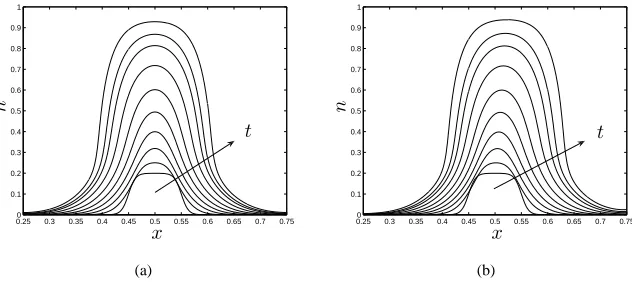
The results presented in figure 3 illustrate how the initial cell distribution given by (3.2) evolves under the influence of perfusion. In figure 3(a), where there is no imposed flow (static culture:Pu =Pd = 0), the cell population grows and spreads symmetrically

in response to the net growth rate,km−kd, and diffusion. This is in direct contrast to the

0.250 0.3 0.35 0.4 0.45 0.5 0.55 0.6 0.65 0.7 0.75 0.1

0.2 0.3 0.4 0.5 0.6 0.7 0.8 0.9 1

n

t

x

(a)

0.250 0.3 0.35 0.4 0.45 0.5 0.55 0.6 0.65 0.7 0.75 0.1

0.2 0.3 0.4 0.5 0.6 0.7 0.8 0.9 1

n

t

x

(b)

Figure 3: Evolution of the cell volume fractionnfor (a) static culture: Pu = Pd = 0,

(b) perfusion: Pu = 1,Pd = 0.1, att = 0−0.297(in steps oft = 0.033). Parameter

values:km= 7.5,kd= 0.1,D= 0.01,θ= 0.97,ν =χ= 0.3,δa=δb= 0.1,µn = 1.3,

a= 0.25,b= 0.75.

both static and perfusive culture (see§1 for details). Figure 3(b) illustrates the effect of perfusion on the cell phase: the tissue is advected by a small amount along the channel by the flow and an accumulation of the cell phase is observed atx=b. Advection may be enhanced by increasing the driving pressure gradient. The cell phase profiles in figure 3 indicate that spreading occurs before the threshold valuesnˆ_{= (θν/(δa+ν), θχ/(δb+χ))}

(at whichΣnandψnschange sign, corresponding to cell-cell and cell-scaffold repulsion;

see (2.17) and the parameter values given in figure 3) due to the presence of diffusion in the model; whennexceeds this value, diffusion is enhanced by repulsive forces between cells which cause the cells to spread more rapidly and produce a more uniform cell den-sity profile at the construct centre. This phenomenon is further investigated in§3.3 by employing simplified forms for the functionsΣn, andψnsto facilitate analytical progress.

Figure 4 shows the influence of the cell population on the culture medium pressure. Up- and downstream from the centrally-located dense population, equation (2.22) supplies

∂2_p

w/∂x2 ≈0 (sincenis small) so we obtain an approximately linear pressure profile;

in-0.25 0.3 0.35 0.4 0.45 0.5 0.55 0.6 0.65 0.7 0.75 0.4

0.5 0.6 0.7 0.8 0.9 1

pw

x

t

(a)

0.250 0.3 0.35 0.4 0.45 0.5 0.55 0.6 0.65 0.7 0.75 0.1

0.2 0.3 0.4 0.5 0.6 0.7 0.8 0.9

pw

x t

(b)

Figure 4: Evolution of the culture medium pressure for (a) early times (smalln): t = 0−0.231(in steps of t = 0.033); and (b) later times (larger n): t = 0.25,0.27,0.29, under perfusion. Parameter values as in figure 3(b).

0.25 0.3 0.35 0.4 0.45 0.5 0.55 0.6 0.65 0.7 0.75 0.35

0.4 0.45 0.5 0.55 0.6 0.65 0.7 0.75 0.8

pn

x t

(a)

0.25 0.3 0.35 0.4 0.45 0.5 0.55 0.6 0.65 0.7 0.75 0.3

0.35 0.4 0.45 0.5 0.55 0.6 0.65 0.7 0.75 0.8

pn

x t

(b)

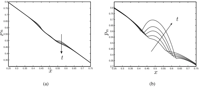
Figure 5: Evolution of the cell pressure for (a) early times (smalln):t= 0−0.13(in steps oft= 0.033); and (b) later times (largern):t= 0.21−0.29(in steps oft= 0.02), under perfusion. Parameter values as in figure 3(b).

terphase pressure functionsΣn,ψns(see equations (2.17) and (2.22)) dominating at low

As the cells repel each other, mass conservation demands that culture medium be drawn in to fill the void, corresponding to the reduction inpw. At the periphery, where the cell

population remains sparse, cell aggregation and attachment is reflected in an increase in

pw.

In figure 5 we compare the cell phase pressure for low and high cell phase density. Recall,pnis influenced bypwand intraphase and interphase interactions:pn=pw+Σn+

(1−θ)ψns. Whennis small, the behaviour is dominated by aggregation (Σn, ψns<0)

and a small decrease in the cell phase pressure is observed. At later times (see figure 5(b)), asnincreases, the contribution from the repulsive terms becomes important (Σn, ψns>0)

and a sharp increase in cell pressure is observed.

0.25 0.3 0.35 0.4 0.45 0.5 0.55 0.6 0.65 0.7 0.75 −0.05

0 0.05 0.1 0.15 0.2

t=0.03 t=0.06 t=0.1

un

|y=

1

/

2

x

t

(a)

0.25 0.3 0.35 0.4 0.45 0.5 0.55 0.6 0.65 0.7 0.75 −0.2

−0.1 0 0.1 0.2 0.3 0.4

un

|y=

1

/

2

x

t

(b)

Figure 6: Evolution of the cell velocity at the channel centreline for (a) early times (small

n): t = 0.033,0.066,0.1; and (b) later times (largern): t = 0.2,0.23,0.25,0.27under perfusion. Parameter values as in figure 3(b).

The velocity of the cell phase (un) at the channel centreline is depicted in figure 6.

For low cell density, aggregation and attachment dominate (Σn, ψns<0) and we observe

that cells move preferentially towards the centre to form a dense aggregate which moves downstream due to the imposed flow (figure 6(a)). As the cell volume fraction increases, repulsive effects become important (Σn, ψns>0) as described above. This effect is

0.25 0.3 0.35 0.4 0.45 0.5 0.55 0.6 0.65 0.7 0.75 −0.05

0 0.05 0.1 0.15 0.2 0.25 0.3

uw

y

=

1

/

2

x

t

(a)

0.25 0.3 0.35 0.4 0.45 0.5 0.55 0.6 0.65 0.7 0.75 −0.8

−0.6 −0.4 −0.2 0 0.2 0.4 0.6 0.8 1

uw

y

=

1

/

2

x

t

(b)

Figure 7: Evolution of the culture medium velocity at the channel centreline for (a) early times (smalln):t= 0.033−0.165(in steps oft= 0.033); and (b) later times (largern):

t= 0.25,0.27,0.29, under perfusion. Parameter values as in figure 3(b).

fraction which is small in these simulations. The aggregative behaviour described above is therefore dominated by cell-cell interactions.

Figure 7 shows the centreline value of the parabolic culture medium velocity profile. The flow profile remainsx-independent prior to, and after, the densely-populated region, under the influence of the linear driving pressure gradient. For both low (figure 7(a)) and high (figure 7(b)) cell phase density, we observe that the flow speed is decreased from the upstream ambient flow velocity as the culture medium encounters the cell popula-tion; near the downstream periphery, an increase to the ambient flow is observed. At low cell density, the culture medium flow increases monotonically between the up- and downstream peripheries. As the density increases, the fluid flow between these peripheral regions changes markedly, reversing flow direction. This is due to the switch between ag-gregative and repulsive behaviour of the cell phase described above; to conserve mass, the culture medium velocity exhibits the opposite behaviour, being drawn into the construct’s centre when cells repel each other.

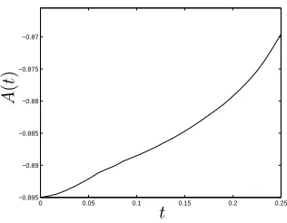
Figure 8 shows the evolution ofA(t), which determines the culture medium pressure and its gradient inx6aandx>b(see equation (2.26)). The magnitude of the pressure gradient decreases with time, causing the up- and downstream flow speed to reduce; we attribute this to the increase of cell volume fraction which fills available pore space and provides increased resistance to flow.

0 0.05 0.1 0.15 0.2 0.25 −0.895

−0.89 −0.885 −0.88 −0.875 −0.87

A

(

t

)

t

Figure 8: Evolution of the functionA(t). Parameter values as in figure 3(b).

predicted by the two-fluid model of O’Dea et al. (2008): consideration of cell-cell and cell-scaffold interactions, together with relaxation of the large drag assumption, results in starkly different behaviour to that found in O’Dea et al. (2008) in which axially asymmet-ric growth was predicted both in static and perfusive conditions (§1). Additionally, since in O’Dea et al. (2008) the limit of large viscous drag is employed, each phase moves with a common velocity and very low perfusion rates are required to prevent cells from being flushed from the scaffold. The results presented here suggest that aggregation in regions of sparse cell density acts to curtail advection, leading to movement of cells towards the cen-tre of the aggregate; furthermore, due to mass conservation, the cell and culture medium velocities exhibit opposite behaviour. Inspection of the model equations has revealed that

forn < θν/(δa+ν)orθχ/(δb+χ), the cell behaviour is dominated by cell aggregation,

with contributions from cell-scaffold attachment being small.

3.2

Asymptotically-small cell density

The results from the numerical scheme may be validated by considering the limit of asymptotically-small cell phase volume fraction, in which case we may construct ana-lytic solutions to the simplified versions of (2.21) and (2.22) (withSn defined by (3.1)).

Choosing

n(x, t) =δn1(x, t) +δ2_{n2(x, t) +· · ·, (3.3)}

where0< δ≪1, we obtain the following system of linear PDEs:

∂n1

∂t +γ

∂n1

∂x = (km−kd)n1+D

∂2_n 1

∂x2 , (3.5)

∂2_p 0

∂x2 = 0,

∂2_p 1

∂x2 =−β

∂n1

∂x , (3.6 a,b)

whereγandβare defined as follows:

γ=− 1

12µn

∂p0

∂x, β=

µ θ

∂p0

∂x. (3.7 a,b)

Considering (2.27)–(2.29) and employing the additional expansion

A(t) =A0(t) +δA1(t) +· · · , (3.8)

it may be shown that appropriate boundary conditions are: atO(1)

∂p0 ∂x

_x=a,b=

A0

θ , p0

_x=a=A0a+Pu

θ , p0

_x=b =A0(b−1) +Pd

θ ; (3.9)

atO(δ):

∂n1 ∂x

x=a,b

=− A0n1

12θµnD

, ∂p1

∂x

x=a,b

=A1

θ +

A0n1

θ2 +

12D θ

∂n1

∂x ,(3.10 a,b)

p1

_x=a= A1a+ (1−θ)χn1

θ , p1

_x=b=A1(b−1) + (1−θ)χn1

θ . (3.11 a,b)

We therefore have four conditions on each of the pressuresp0,p1; two of which are

im-posed as boundary conditions, the remaining equations being used to calculateA0andA1.

As previously, the overspecification of the functionsA0,A1results from the imposition of

continuity of total flux. When satisfied, the additional conditions guarantee continuity of flux.

For simplicity, we consider the solution of equations (3.5) and (3.6) in the limitD= 0, for which the interface between the cell phase and the surrounding culture medium is sharp. The cell population is then confined within two moving boundaries,x=l(t), r(t),

within the scaffold regiona6x6b.

It is trivial to show thatA0=Pd−Puand the leading-order pressure,p0, is given by

p0(x, t) = (Pd−Pu)x+Pu

We may now proceed with the solution of equation (3.5) withD= 0since the constant,γ, is given by equation (3.7a). We first specify an appropriate initial cell phase distribution as follows:

n1(x,0) =

(

n(x) l(0)6x6r(0),

0 otherwise, (3.13)

whereinn(x)is an as yet unspecified function andx=l(0), r(0)are the initial positions of the interfacesl(t),r(t); (3.10a) is redundant sincen1 = 0fora6x < l,r < x6b.

The solution,n1(x, t)takes the form of a travelling-wave:

n1(x, t) =

(

n(x−γt)e(km−kd)t _l(t)

6x6r(t),

0 otherwise, (3.14)

wherel(t) = l(0) +γt, r(t) = r(0) +γt, representing exponential growth of a cell population at a ratekm−kdwhich is advected along the channel at speedγ. This behaviour

is valid for the very early stages of cell growth during which behaviour is dominated by uniform proliferation and cell spreading is negligible.

The correction to the culture medium pressurep1is given by equation (3.6b), and, in

addition to the conditions (3.9)–(3.11) atx=a, b, must obey the following jump condi-tions acrossx=l(t), r(t):

[θp1]+₋ = [χ(1−θ)n1]+,

θ∂p1

∂x

+

−

=

(Pu−Pd)µn1

θ

+

, (3.15 a,b)

where[..]+ _and[..]− _{denote the limiting values from the cell/culture medium/scaffold}

region (l(t)6x6r(t)) and the culture medium/scaffold regions (a6x < l(t),r(t)< x6b), respectively and[..]+₋denotes the jump across either interface.

To determine the correction to the pressure in the culture medium, we must specify the initial cell phase distribution,n(x). For simplicity we choosen(x) = ˆn, wherenˆis constant. We obtain:

p1(x, t) =

      

e

P ekt_{[l(t)−r(t)]x a6x < l(t),}

e

P ekt_{[1 +l(t)−r(t)]x+e}kt_{(χ−P le (t)) l(t)6x6r(t),}

e

P ekt[l(t)−r(t)] (x−1) r(t)< x6b,

(3.16)

wherek=km−kd,χ=χ(1−θ)ˆn/θ,µ= 1/µn−1andPe= (Pu−Pd)µˆn/θ2.

The evolution of the cell volume fraction,n1, is shown in figure 9. The corresponding

pressure correction,p1, and the culture medium pressure (toO(δ)accuracy)pw =p0+

δp1, are shown in figure 10. The correction to the pressure (p1) is an order of magnitude

10(b), the small parameter is chosen to beδ = 1. With the exception of the diffusion coefficient,D, the parameter values are chosen to be the same as those used in§3.1.

0.250 0.3 0.35 0.4 0.45 0.5 0.55 0.6 0.65 0.7 0.75 0.1

0.2 0.3 0.4 0.5 0.6 0.7 0.8 0.9

x

t

n1

Figure 9: Evolution of the cell volume fraction,n1, under perfusion att = 0−0.2(in

steps oft= 0.04).D= 0,δ= 1, other parameter values as in§3.1.

0.25 0.3 0.35 0.4 0.45 0.5 0.55 0.6 0.65 0.7 0.75 −0.01

−0.005 0 0.005 0.01 0.015 0.02

x t

p1

(a)

0.4 0.42 0.44 0.46 0.48 0.5 0.52 0.54 0.56 0.58 0.6 0.45

0.5 0.55 0.6 0.65 0.7

x t

pw

(b)

Figure 10: Evolution of (a) the pressure correction,p1and, (b) the culture medium

pres-sure,pw=p0+δp1in a magnified region withina6x6b, under perfusion att= 0−0.2

(in steps oft= 0.04). Parameters as in figure 9.

As noted above, the solution in the sharp interface limit predicts that the cell population grows exponentially with growth ratekm−kd, while being advected along the channel at

0.01 0.02 0.03 0.04 0.05 0.06 0.07 0.08 0.09 0.501

0.502 0.503 0.504 0.505 0.506

p

o

si

ti

o

n

δ

t

(a)

0 0.01 0.02 0.03 0.04 0.05 0.06 0.07 0.08 0.09 0.1 0

0.02 0.04 0.06 0.08 0.1 0.12

%

re

la

ti

v

e

er

ro

r

δ

t

(b)

Figure 11: (a) Comparison of the numerically-computed position of the maximum value ofn(–) compared to the predicted position of the travelling wave (- -) and, (b) the % relative error between the calculated and predicted position forδ = 1/25,1/5,1. The arrows indicate the direction of increasingδ.

predicted by the travelling-wave solution (3.14), and figure 11(b) depicts the % relative er-ror between the numerically-calculated and analytically-predicted positions over time for different values of the small parameterδ. Asδis decreased, the numerical prediction for the advection speed approachesγ, and the % relative error decreases (forδ= 1/25, the % error isO(10−2_)).

The perturbation (p1) to the culture medium pressure is found to be piecewise linear,

with positive gradient in the up- and downstream regions where n1 = 0 and negative

gradient where cells are present (l(t) 6 x 6 r(t)). Upstream, the sharp interface limit predicts a small increase to the leading-order pressure; downstream, a small decrease is observed. Comparison of the predicted pressure shown by figure 10(b) and the culture medium pressure calculated in §3.1 (figure 4(a)) shows qualitative agreement. Further-more, considering the boundary conditions (2.27a) and (2.28a) and the behaviour ofA(t)

(see figure 8 which indicates thatA(t) <0and that|A(t)|decreases with time), we see that atx = athe culture medium pressure increases over time; at x = b, the pressure decreases. This behaviour is evident from figure 10(b), indicating that the culture medium pressure (pw=p0+δp1) predicted in this asymptotic limit reproduces that of the system

(2.21), (2.22), (2.27)–(2.29) when the cell density isO(1).

analytic solutions using Greens functions for the caseD >0.

3.3

Analysis of a simplified model of cell-cell and cell-scaffold

inter-action

To investigate further the effect of intraphase pressure and interphase traction on cell be-haviour, especially the switch between aggregative and repulsive behaviour observed in the numerical simulations (see figures 4–7), we now simplify the intraphase pressure and in-terphase traction functions defined by equations (2.17), replacing them with the following piecewise-constant forms:

Σn(n) =

(

−ν n < NΣ,

δa n>NΣ,

ψns(n) =

(

−χ n < Nψ,

δb n>Nψ,

(3.17)

whereNΣ,Nψare the threshold values at which repulsive forces between cells dominate

those associated with aggregation and at which the cells become repelled from the scaffold, respectively. For simplicity, in the following we setNΣ=Nψ =Nand we further assume

that the viscosities of the culture medium and cell phases are equal (µn= 1). Under these

simplifications, equation (2.22) reduces to:

θ∂

2_p

w

∂x2 =

(

ν ∂2

n

∂x2 n < N,

−δa ∂

2

n

∂x2 n>N.

(3.18)

Assumingn < Natx=a, b, the corresponding boundary conditions (2.27)–(2.29) are

pw

_x=a= Aa+Pu+αn

θ , ∂pw ∂x

_x=a,b=

A+ 12D∂n

∂x

θ−n , (3.19 a,b)

pw

x=b=

A(b−1) +Pd+αn

θ , ∂n ∂x

x=a,b

= An

(θ−n)(ν−12D)−12Dn, (3.20 a,b)

whereα=ν+ (1−θ)χ.

We proceed by considering separately the regions in whichn < N andn > N, as-suming thatn,∂n/∂x,pwand∂pw/∂xare continuous atn=N. Equations (3.18)–(3.20)

yield expressions for the culture medium pressure in each region, substitution of which into (2.21) yields nonlinear advection-diffusion equations for the cell volume fraction (omit-ted), in which the effective diffusion coefficients are defined:

D=D−(θ−n)ν

12θ , n < N; D(n) =D+

(θ−n)δa

12θ , n>N. (3.21)

into the behaviour of the cells: the modified diffusion coefficients, indicate that when ag-gregation dominates (n < N), the diffusive transport of the cells is reduced; conversely, when n > N, repulsive effects dominate and the cellular diffusion coefficients are in-creased.

Aggregation-enhanced cell behaviour is most clearly illustrated by considering the cell phase velocity defined by (2.19b). In view of the simplified forms (3.17), we find that the cell velocity at the channel centreline forn < Nis given by

un≈ −

1 8µn

_∂p

w

∂x −

ν n

∂n ∂x

, (3.22)

so that for smalln, the second term dominates and cells tend to move up gradients of cell density.

3.4

Summary

In this section, we have considered the uniform growth of a tissue construct. We presented numerical simulations which indicate that the consideration of interactions between ad-jacent cells and between cells and the scaffold leads to distinctly different cell behaviour as the construct density increases: cell aggregation and attachment being replaced by re-pulsion. The accuracy of the numerical simulations was established by constructing ana-lytic solutions in the limit of asymptotically-small cell density. To further investigate the behavioural switch observed in the numerical simulations, we employed simplified func-tional forms for the cell-cell and cell-scaffold interactions. Our analysis indicated that the cells’ diffusive behaviour is reduced or augmented depending upon the relative importance of cell aggregation and repulsion.

4

Mechanotransduction

The relevance of our modelling framework hinges on the appropriate choice ofSn; we

pause here to highlight an important restriction on its form. Equation (2.21) is derived by averaging the conservation of mass equation for the culture medium phase (in the trans-verse direction), implyingSn = Sn(x, t); consequently, explicit coupling between the

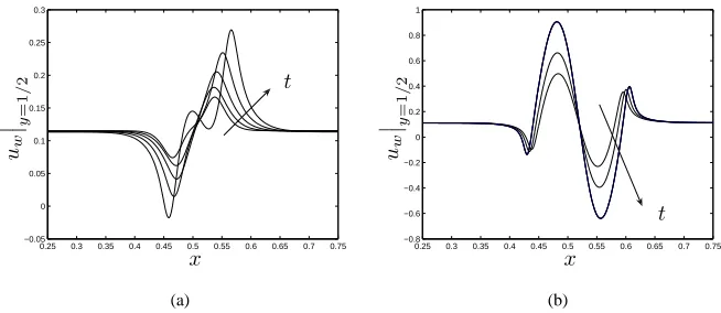
shear stress induced by the flow of culture medium (which is dependent ony) and the cell growth response is prohibited. The gross effect of this coupling may still be incorporated by noting that the averaged flow-induced shear stress experienced by the cells is propor-tional to the culture medium velocity. In view of equation (2.19a), we therefore model the shear stress as being proportional to the gradient of the culture medium pressure. In the following, we consider in turn the following choices:Sn(n),Sn(n, pn),Sn(n,|∂pw/∂x|).

4.1

Cell density dependence:

S

=

S

(

n

)

We identify three distinct stages in the behaviour of the cell population: (i) a proliferative stage,Sn =k1nn; (ii) an ECM-producing stage,Sn =k2nn; and (iii) an apoptotic stage,

Sn=−kdn. These represent the effects of contact inhibition and residual stresses caused

by growth on the phenotypic progression of cells. Contact inhibition and high stress levels inhibit cell division, whilst a moderate level of stress appears to enhance tissue growth (Chaplain et al., 2006; Roose et al., 2003). We therefore choosek2n> k1nso that the rate

of cell phase growth is increased during the ECM-production phase; we remark here that since the cell phase comprises cells and ECM, it is not possible to distinguish between cell proliferation and ECM deposition or cell death and ECM degradation in this model. For simplicity, we assume that the rates of growth and death (k1n, k2n, kd) are constant. The

threshold cell densities that separate these three types of behaviour are denotedn′

1andn′2.

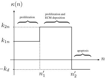
We employ step functions to represent this behaviour; the net rate of growth and death of the cell phase, denotedκ(n), is illustrated by figure 12 and is related toSnas follows:

Sn(n) =k1nH(n′1−n) +k2nH(n−n′1)−(k2n+kd) H(n−n′2)

n=κ(n)n, (4.1)

whereH(n) is the Heaviside step function and without loss of generality, we specify

κ(n) =k2nat the threshold valuesn=n′1,n′2. Step functions for density- and

nutrient-dependent growth have been employed by Byrne & Preziosi (2003a) in which the switch between two density-dependent responses was modelled; a (mollified) piecewise constant response was employed by Chaplain et al. (2006). Here, we consider three distinct growth phases in each of which the proliferative rate is constant.

n

n′

1 n′2

κ(n)

k1n

k2n

−kd

proliferation

apoptosis proliferation and

ECM deposition

z }| { z }| {

z }| {

Figure 12: Schematic representation of the progression of the cells from a proliferative phase to an apoptotic phase, via an ECM-producing phase in response to the local cell density.

responses occur. The corresponding culture medium and cell phase pressures are shown in figures 13(b) and 14. The velocity of each phase at the channel centreline is shown in figure 15; for clarity, only the velocities arising at later times, oncenhas reached the threshold valuen=n′

2at some point in the domain, are shown.

0.250 0.3 0.35 0.4 0.45 0.5 0.55 0.6 0.65 0.7 0.75 0.1

0.2 0.3 0.4 0.5 0.6 0.7

n

t

x

(a)

0.25 0.3 0.35 0.4 0.45 0.5 0.55 0.6 0.65 0.7 0.75 0.3

0.35 0.4 0.45 0.5 0.55 0.6 0.65 0.7 0.75 0.8

pw

t

x

(b)

Figure 13: The evolution of (a) the cell volume fraction,n < n′

1andn > n′2, (–);n′1 6

n6 n′

2, (· · ·) and, (b) the pressure of the culture medium, att = 0−0.35(in steps of

t≈0.038) for growth behaviour defined by (4.1) and perfusive culture:Pu= 1,Pd= 0.1,

k1n = 6.5,k2n= 7.5,kd= 1,D= 0.01,θ= 0.97,n′1= 0.4,n′2= 0.6.

Inspection of figure 13(a) reveals that the growth of the cell phase ceases whenn=n′

2,

0.25 0.3 0.35 0.4 0.45 0.5 0.55 0.6 0.65 0.7 0.75 0.35 0.4 0.45 0.5 0.55 0.6 0.65 0.7 0.75 0.8 pn x t (a)

0.25 0.3 0.35 0.4 0.45 0.5 0.55 0.6 0.65 0.7 0.75 0.35 0.4 0.45 0.5 0.55 0.6 0.65 0.7 0.75 0.8 pn x t (b)

Figure 14: The evolution of the pressure of the cell phase for (a) early times (smalln:

t = 0−0.15, in steps oft = 0.0375) and, (b) later times (largern: t = 0.2−0.35in steps oft= 0.05), for growth behaviour defined by (4.1) and perfusive culture. Parameter values as per figure 13.

0.25 0.3 0.35 0.4 0.45 0.5 0.55 0.6 0.65 0.7 0.75 −0.05 0 0.05 0.1 0.15 0.2 0.25 0.3 uw

|y=

1 / 2 x t t (a)

0.25 0.3 0.35 0.4 0.45 0.5 0.55 0.6 0.65 0.7 0.75 −0.2 −0.1 0 0.1 0.2 0.3 0.4 un

|y=

1 / 2 x t t (b)

Figure 15: The evolution of (a) the velocity profile of the culture medium, (b) the velocity profile of the cell phase (at the channel centreline), att= 0.2−0.35(in steps oft= 0.05) for growth behaviour defined by (4.1) and perfusive culture. Parameter values as per figure 13.

density of the cell phase does not fall belown=n′

2. Figures 13(b), 14 and 15 indicate that

flow. Some repulsion is evident in figure 14(b); however, the behaviour shown in 5(b) is prevented by curtailed cell phase growth. Similarly, the dramatic flow reversal observed in figures 6(b) and 7(b) does not occur (limited upstream flow of culture medium due to cell aggregation is observed at the upstream periphery of the construct, as in figure 7(a)); rather, the flow attains a constant value in the region wheren=n′

2.

4.2

Cell density and pressure dependence:

S

=

S

(

n, p

)

An alternative way to model the tendency of cells to adapt their behaviour in response to their local density is to consider the pressure of the cell phase as an indicator of cell density; i.e.Sn(n, pn). Sincepn is intimately connected to the pressure of the culture

medium, this choice has the added advantage of including the response of cells to the local fluid dynamics.

We model the cells’ pressure-dependent response in a similar manner to that outlined above and assume that at intermediate pressure, the cells exhibit enhanced proliferation and ECM deposition; at low pressure, the cells enter a state of relative quiescence in which proliferation and ECM deposition are greatly reduced; at high pressure, the cells become apoptotic. This behaviour is consistent with Roelofsen et al. (1995) in which it was reported that excessive hydrostatic pressure (> 200kPa) has an inhibitory effect on bone-specific gene expression in murine osteoblast-like cells. Introducing threshold cell pressures at which the cell proliferation is heightened (p′

n1) and apoptosis is stimulated

(p′

n2), we represent the mass transfer term with step functions, as defined below and

illus-trated by figure 16(a):

Sn(n, pn) =k1pH(p′n1−pn) +k2pH(pn−p′n1)−(k2p+kd) H(pn−p′n2)

n=κ(pn)n.

(4.2) Within our numerical scheme we chooseκ(pn) =k2patpn=p′n1, p′n2.

Comparison of figures 13(a) and 16(b) demonstrates the effect ofSn(n, pn)on the

growth of the cell phase: rather than being arrested at a threshold density, the growth of the cell phase is skewed towards the downstream boundaryx= b. This is due to the interplay between the imposed pressure,pw, (which dominatespnwhennis small) and the

repulsive intraphase pressure and interphase traction contributions (which cause a dramatic increase inpnwhennbecomes larger; see equation (2.17)). Growth of the cell phase near

x=ais inhibited because the culture medium pressure is high there(κ(pn) =−kd); near

x=b, growth is reduced(κ(pn) =k1p< k2p); and between these two regions, enhanced

growth is initially observed until the cell pressure achieves the thresholdp′

pn

p′

n1 p′n2

κ(pn)

k2p

k1p

−kd

quiescence

apoptosis proliferation and

ECM deposition

z }| { z }| {

z }| {

(a)

0.25 0.3 0.35 0.4 0.45 0.5 0.55 0.6 0.65 0.7 0.75 0 0.1 0.2 0.3 0.4 0.5 0.6 0.7 0.8 n t x (b)

Figure 16: (a) Schematic representation of the progression of the cells from a quiescent phase to an apoptotic phase, via a proliferative phase in response to the pressure of the cell phase,pn; (b) the evolution of the cell volume fraction att = 0−0.28(in steps of

t= 0.02),pn > p′n2, (-.-);p′n1 6pn 6p′n2, (–);pn < p′n1, (· · ·), for growth behaviour

defined by (4.2) and perfusive culture:Pu = 1,Pd = 0.1,k1p = 4,k2p = 7.5,kd = 2,

D= 0.01,θ= 0.97,p′

n1= 0.35,p′n2= 0.6.

0.25 0.3 0.35 0.4 0.45 0.5 0.55 0.6 0.65 0.7 0.75 0.3 0.35 0.4 0.45 0.5 0.55 0.6 0.65 0.7 0.75 0.8 pw x t (a)

0.25 0.3 0.35 0.4 0.45 0.5 0.55 0.6 0.65 0.7 0.75 0.3 0.35 0.4 0.45 0.5 0.55 0.6 0.65 0.7 0.75 0.8 pw x t (b)

Figure 17: The evolution of the pressure of the culture medium for (a) early times (small

n): t = 0−0.2(in steps oft = 0.04), (b) later times (largern): t = 0.22−0.28(in steps oft= 0.02), for growth behaviour defined by (4.2) and perfusive culture. Parameter values as per figure 16.

line in figure 16). Comparison between figures 5 and 18 shows that the cell pressure is not dramatically affected by this changed cell distribution until the upper thresholdp′

n2

0.25 0.3 0.35 0.4 0.45 0.5 0.55 0.6 0.65 0.7 0.75 0.35

0.4 0.45 0.5 0.55 0.6 0.65 0.7 0.75 0.8

pn

p′

n1

p′

n2

x t

(a)

0.25 0.3 0.35 0.4 0.45 0.5 0.55 0.6 0.65 0.7 0.75 0.3

0.4 0.5 0.6 0.7 0.8

pn

p′

n1

p′

n2

x t

(b)

Figure 18: The evolution of the pressure of the cell phase for (a) early times (smalln):

t= 0−0.12(in steps oft= 0.4), (b) later times (largern): t= 0.16−0.28(in steps of

t= 0.03), for growth behaviour defined by (4.2) and perfusive culture. Parameter values as per figure 16.

0.25 0.3 0.35 0.4 0.45 0.5 0.55 0.6 0.65 0.7 0.75 0

0.1 0.2 0.3 0.4 0.5 0.6 0.7 0.8

n

t

x

Figure 19: The evolution of the cell volume fraction att= 0−0.3(in steps oft= 0.033),

pn < p′n1,pn > p′n2, (-);p′n1 6pn 6p′n2, (· · ·), for growth behaviour defined by (4.2)

and static culture: Pu = 0 = Pd,k1p = 7.5,k2p = 9,pn1 = 0,p′n2 = 0.01, other

parameters as in figure 16.

preventspnfrom exceedingp′n2(see the last line in figure 18(b)). Similarly, figures 4 and

17 show that the culture medium pressure is qualitatively similar to that found previously. For brevity, the velocities of each phase are not given here since (except at late times) they will be qualitatively similar to those found in§3.1.

growth results in a construct whose composition is qualitatively similar to that resulting from density-regulated growth. Comparison with figure 13(a), which depicts the construct morphology resulting from density-regulated growth under perfusion, shows that the con-structs may be distinguished by the asymmetry introduced by the flow. Qualitatively in-distinguishable constructs are obtained in static conditions (results omitted).

Using a two phase model, O’Dea et al. (2008) have also demonstrated that in the absence of perfusion, cell density and pressure-mediated growth result in indistinguishable constructs; the similarity of the constructs produced was a consequence of the simplified model in which the pressure was directly proportional to the cell distribution. In this three phase model, where the relationship between the cell phase distribution and its pressure is more complex, the net result is the same; however, the mechanism is different. In static culture, dominance of the aggregation and scaffold affinity parameters at low cell density ensures thatpn <0and tissue growth is determined by the reduced growth rate,

κ(pn) =k1p; as the density increases, the repulsive terms become important, causing an

increase in cell phase pressure untilpnachieves the upper threshold and the cells become

apoptotic, preventing the cell density from further increase. Cells near the periphery of the aggregate (where the density and associated cell pressure are lower) proliferate at a rate

k1pork2pdepending upon the value ofpn(cells proliferating atκ(pn) =k2pare indicated

by the dotted line in figure 19). Eventually, these cells achieve sufficiently high density to cause the pressure to attain the upper threshold, resulting in curtailed growth. In this way, a construct whose density is approximately uniform is attained. We note that these results were obtained for the casePu=Pd = 0; similar behaviour is obtained forPu=Pd >0

depending upon the choice of thresholdsp′

n1, p′n2.

4.3

Shear stress dependence:

S

=

S

(

n,

∂p

/∂x

)

We now consider the effect of coupling the growth of the cell phase to the shear stress induced by the external fluid dynamics; i.e.Sn(n,

∂pw/∂x

the mass transfer term,Sn(n,∂pw/∂x)defined as follows, and depicted in figure 20(a): Sn n, ∂pw ∂x =

−k1τ−k2τ

2

tanh

g∂pw

∂x

−P1′

−1

−k2τ+kd

2 tanh g

∂p_∂xw

−P2′

−1

−kd

n =κ ∂pw ∂x n. (4.3)

In (4.3), the threshold values at which the rate of cell proliferation and ECM deposition are heightened and the necrotic phase is entered are denotedP′

1andP2′ respectively and the

parameter,g, determines the closeness of the approximation to the step-function behaviour used previously.

Inspection of figures 20 and 21 shows how the cell phase is affected by shear-dependent proliferation. When the cell population is relatively small, disturbance to the culture medium flow is minimal and the shear remains within the proliferative region: P′

1 6

∂pw/∂x

6P′

2. As the cell population increases, the increased construct density causes

a reduction inuwnear the upstream periphery, and an increase downstream (see figure

7(a)), causing the upstream shear to fall below theP′

1threshold and resulting in decreased

proliferation there (figure 21(a)). A further increase in the cell population causes the flow disturbance to increase (see figure 7(b)) resulting in flow reversals at a number of points within the domain. This causes the shear to increase to theP′

2threshold and to cross theP1′

threshold repeatedly (see figure 21(b)), resulting in cell phase death and reduced cell phase growth at various regions within the cell population, leading to highly heterogeneous con-struct composition. Inspection of figures 20(b) and 21(b) shows that the influence of fluid shear stress on cell phase growth is clearest at late times. The high level of shear near the construct centre and reduced shear near the upstream periphery causes cell phase growth to be skewed in the downstream direction.

5

Discussion

k2τ

kd

k1τ

κ(∂pw

∂x ) ∂pw ∂x P′

1 P2′

quiescence

apoptosis proliferation and

ECM deposition

z }| { z }| {

z }| {

(a)

0.25 0.3 0.35 0.4 0.45 0.5 0.55 0.6 0.65 0.7 0.75 0 0.1 0.2 0.3 0.4 0.5 0.6 0.7 0.8 n x t (b)

Figure 20: (a) Schematic representation of the progression of the cells from a quiescent phase to an apoptotic phase, via a proliferative phase in response to the flow-induced shear stress; (b) the evolution of the cell volume fraction,pwx

< P′

1, (-.-);P1′ 6

pwx

6P′

2,

(–);pwx

> P′

2, (· · ·), att= 0−0.4(in steps oft= 0.05) for growth behaviour defined

by (4.3) and perfusive culture:Pu= 1,Pd= 0.1,km= 7.5,km= 4,kd= 2,D= 0.01,

θ= 0.97,P′

1= 0.5,P2′= 1.5,g= 60.

0.25 0.3 0.35 0.4 0.45 0.5 0.55 0.6 0.65 0.7 0.75 −1.6 −1.4 −1.2 −1 −0.8 −0.6 −0.4 −0.2 0 P′ 1 P′ 2 ∂

pw _∂x

x

t

(a)

0.25 0.3 0.35 0.4 0.45 0.5 0.55 0.6 0.65 0.7 0.75 −2 −1.5 −1 −0.5 0 0.5 P′ 1 P′ 2 ∂

pw _∂x

x t

(b)

Figure 21: The evolution of the pressure gradient of the culture medium for (a) early times (smalln: t = 0.02−0.22in steps oft = 0.05), (b) later times (largern: t = 0.25,0.3.0.35), for growth behaviour defined by (4.3) and perfusive culture. Parameter values as per figure 20.