5University of Michigan, 1517 Space Research Building, Ann Arbor, MI 48109-2143, USA
Accepted 2013 January 29. Received 2013 January 23; in original form 2012 December 11
A B S T R A C T
The large-scale field of the Sun is well represented by its lowest energy (or potential) state. Recent observations, by comparison, reveal that many solar-type stars show large-scale surface magnetic fields that are highly non-potential – that is, they have been stressed above their lowest energy state. This non-potential component of the surface field is neglected by current stellar wind models. The aim of this paper is to determine its effect on the coronal structure and wind. We use Zeeman–Doppler surface magnetograms of two stars – one with an almost potential, one with a non-potential surface field – to extrapolate a static model of the coronal structure for each star. We find that the stresses are carried almost exclusively in a band of unidirectional azimuthal field that is confined to mid-latitudes. Using this static solution as an initial state for a magnetohydrodynamic (MHD) wind model, we then find that the final state is determined primarily by the potential component of the surface magnetic field. The band of azimuthal field must be confined close to the stellar surface, as it is not compatible with a steady-state wind. By artificially increasing the stellar rotation rate, we demonstrate that the observed azimuthal fields cannot be produced by the action of the wind but must be due to processes at or below the stellar surface. We conclude that the background winds of solar-like stars are largely unaffected by these highly stressed surface fields. Nonetheless, the increased flare activity and associated coronal mass ejections that may be expected to accompany such highly stressed fields may have a significant impact on any surrounding planets.
Key words: magnetic fields – stars: coronae – stars: winds, outflows.
1 I N T R O D U C T I O N
The magnetic fields of solar-like stars are an important influence not only on the rotational evolution of the stars themselves, but also on the atmospheres and exospheres of any planets that might surround them. This magnetic field not only transfers torques between the protoplanetary disc and the young star, but it also governs the loss of angular momentum in a wind. Any orbiting planets are exposed to the erosive effects of this wind and also the coronal X-ray emission from the star (Khodachenko et al. 2007).
Both of these effects are likely to weaken as the star ages and spins down, generating less magnetic flux and hence producing a weaker wind and reduced X-ray emission (G¨udel 2004). Recent maps of the surface magnetic fields of stars with a range of masses and rotation rates, however, suggest that it is not only the strength
E-mail: [email protected]
of the magnetic field that changes with rotation rate, but also its geometry (Donati et al. 2008; Morin et al. 2008; Petit et al. 2008; Morin et al. 2010). In contrast to the Sun which shows spots in well-defined ‘active latitudes’, solar mass stars that are still in the rapidly rotating stage typically show very non-solar magnetic fields, with spots that extend over the whole surface, often resulting in a dark polar cap (Strassmeier 2009). Mixed polarity magnetic flux is seen at all latitudes on these stars.
Typically these rapidly rotating stars have X-ray luminosities that are three orders of magnitude greater than that of the Sun, but the extent of the corona that produces this emission is currently unknown. X-ray spectra suggest that their coronae are dense and compact (Dupree et al. 1993; Schrijver et al. 1995; Brickhouse & Dupree 1998; Maggio et al. 2000; G¨udel et al. 2001; Sanz-Forcada, Maggio & Micela 2003). In contrast, the presence of multiple large cool prominences trapped in co-rotation at distances of several stel-lar radii suggests that their closed magnetic fields, if not their X-ray bright coronae, must be very extended (Collier Cameron &
C
2013 The Authors Published by Oxford University Press on behalf of the Royal Astronomical Society
at Library & Information Services, University of St Andrews on August 8, 2013
http://mnras.oxfordjournals.org/
Robinson 1989a,b; Collier Cameron & Woods 1992; Jeffries 1993; Byrne, Eibe & Rolleston 1996; Eibe 1998; Barnes et al. 2000; Donati et al. 2000). One possible explanation is that the promi-nences form not within the X-ray bright corona, but in the cusps of helmet streamers that extend out into the stellar wind (Jardine & van Ballegooijen 2005). These prominences typically form in a time-scale of 1 d and some 1–10 appear in the observable hemisphere at any time. Their ejection in the stellar equivalent of solar coronal mass ejections not only contributes to the angular momentum loss from the star (Aarnio et al. 2011a,b) but it will also temporarily enhance the ram pressure of the stellar wind and hence, the degree of compression of any planetary magnetospheres.
The surface fields of these young stars show one other very non-solar feature and that is the presence of a strong (sometimes dominant) non-potential component (Petit et al. 2008). Stellar winds can of course produce azimuthal fields as the escaping wind extracts angular momentum from the star via magnetic torques, but for slow rotators it is unlikely that this could generate such strong fields at the photospheric level. Several other mechanisms have been proposed to explain the surface azimuthal fields, including the underlying dynamo (Donati & Collier Cameron 1997), and the effect of differential rotation in the presence of a unipolar cap (Pointer et al. 2002).
For solar mass stars, the surface differential rotation is similar to that of the Sun, but for higher-mass stars the differential rotation can be extreme, with equator to pole lap times as short as 16 d (Barnes et al. 2005; Marsden et al. 2005, 2006; Jeffers et al. 2011). The effect that this enhanced shear might have on the coronal and wind dynamics and the possible rate of coronal mass ejections is unknown. For low mass stars the differential rotation is typically weak (Morin et al. 2008). The high flaring rate of these stars however suggests that some dynamic process is stressing the coronal field – even although in many cases the large-scale field that is detected with Zeeman–Doppler imaging (ZDI) is close to its potential or lowest energy state.
Some insight into these stellar fields can be gained by considering the changes in the solar magnetic field over the Sun’s magnetic cy-cle. At minimum, the solar field is closest to an aligned dipole, with fast wind streams emerging from the open field regions at the pole and the slow streams emerging from above the low-latitude active regions. As the cycle progresses, more bipoles emerge, contributing to the azimuthal field. These are acted on by diffusion and differen-tial rotation, and their transport towards the poles by the meridional flow eventually reverses the polar polarity. In addition, their net contribution to the azimuthal field causes the axis of the large-scale dipole to move down into the equatorial plane and eventually re-verse. This growth of active regions (and associated coronal mass ejections) through the cycle is also accompanied by the extension of the polar coronal holes down towards the equatorial plane. As a result, fast wind streams originate at a range of latitudes and may interact with the slow wind streams to produce ‘corotating interac-tion regions’ in the solar wind. These shocks provide a local density enhancement that, combined with the increased number of coronal mass ejections, can modulate the cosmic ray flux at Earth (Wang, Sheeley & Rouillard 2006). Recent models of the variation of the solar wind through its cycle (Pinto et al. 2011) show that the mag-netic torques exerted on the Sun vary significantly through its cycle, giving two orders of magnitude variation in the spin-down time.
By analogy with the Sun, the very active young stars that show predominantly non-axisymmetric and non-potential surface fields may have winds that show a mixture of fast and slow wind streams with coronal mass ejections emerging from a range of latitudes.
In-deed, the fact that these stars typically show mixed-polarity flux at all latitudes may suggest that their winds (while showing some char-acteristics of the solar wind at maximum) are much more extreme than the solar wind.
Most stellar wind models are, however, based on the solar anal-ogy. The simplest early models, such as the traditional Weber– Davies model (Weber & Davies 1967), assumed a split monopole, but more recent work usually initiates magnetohydrodynamic (MHD) simulations from an initial state defined by a ‘potential field source surface’ model (Altschuler & Newkirk 1969; Schatten, Wilcox & Ness 1969). This approach assumes that the field is po-tential (i.e. in its lowest energy state) and that at some height above the surface the field lines are opened up by the pressure of the hot coronal gas. This method uses only the radial field component at the surface, neglecting the azimuthal and meridional components. Its advantage is that it is computationally cheap and it provides a unique solution for the magnetic structure. A recent comparison of the global structure predicted by both the potential field source sur-face method and the full MHD simulation suggests that the former captures the large-scale structure of the solar coronal field fairly reliably (Riley et al. 2006).
This approach would not however capture the non-potential na-ture of the magnetic fields observed at the surfaces of other stars. The purpose of this paper is to explore the effect of this non-potential field on the large-scale structure of the corona and winds of solar-type stars.
2 T H E S U R FAC E M AG N E T O G R A M S
In order to study the effects of the non-potential field on the coronal structure and dynamics, we choose to compare two stars (CE Boo and GJ 49) that are similar in rotation rate but with slightly different masses. One has a surface field that is close to potential, while the other has a significant non-potential component. Both stars are slow rotators, so rotational effects are minimal. In addition, the inclination of the rotation axes of both stars to the line of sight is the same, so the magnetic fields of both stars are seen in the same orientation. The stellar parameters are shown in Table 1.
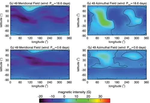
[image:2.595.309.549.678.732.2]We choose initially to compare the static coronal structures that are found by assuming either that the field is purely potential, or that it has both potential and non-potential components. These extrapo-lations can be used as the initial condition for a full MHD solution. Since we are particularly interested in the non-potential field, we also explore the possibility that for the more rapidly rotating stars it is the rotational stressing of the surface field by the action of the wind that causes the field to depart from a potential state. We there-fore perform one simulation of the wind of GJ 49 with an artificially decreased stellar rotation period of 0.6 d and compare this to the wind parameters found with the observed rotation period of 18.6 d.
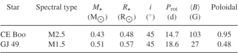
Table 1. Stellar and magnetic parameters for CE Boo and GJ 49, taken from Donati et al. (2008). The table lists sequentially the stellar name, spectral type, mass, radius, inclination of the rotation axis and the rotation period, and then the field properties: the reconstructed magnetic flux density and the fractional energy in the poloidal (potential) field.
Star Spectral type M R i Prot B Poloidal (M) (R) (◦) (d) (G)
CE Boo M2.5 0.43 0.48 45 14.7 103 0.95
GJ 49 M1.5 0.51 0.57 45 18.6 27 0.48
at Library & Information Services, University of St Andrews on August 8, 2013
http://mnras.oxfordjournals.org/
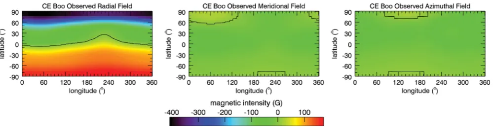
Figure 1. Surface magnetic field maps of CE Boo derived from spectropolarimetric observations (Donati et al. 2008). The single black line shows the zero-field contour that separates regions of opposite polarity.
The input for the static extrapolation is taken from Donati et al. (2008). The surface magnetic field of both stars were modelled with ZDI from time series of spectropolarimetric observations collected over approximately two consecutive stellar rotations. For spatially unresolved sources, due to the mutual cancellation of contributions from neighbouring regions of opposite polarities to the polarized signal, spectropolarimetric measurements can only probe the large-scale component of magnetic fields (see e.g. Morin 2012). The maximum degreeof modes that can be reconstructed with ZDI depends on the star’s projected rotational velocity. For slow rotators such as CE Boo and GJ 49, the reconstruction is limited to modes with order≤8. As there is no unique solution to the ZDI problem, a regularization scheme has to be used. A maximum entropy solution corresponding to the lowest magnetic energy content is used. It is optimal in the sense that any feature present in the map is actually required to fit the data. Although this method does not allow us to derive formal error bars on the reconstructed maps, numerical experiments have shown that ZDI is a robust method (Donati & Brown 1997; Morin et al. 2010).
This reconstructed field is expressed as a sum of a poloidal and toroidal field (Mestel 1999). The poloidal component captures the potential contribution to the total field, that is the component that is in its lowest energy state. The toroidal component lies on the surfaces of concentric spheres and captures the non-potential com-ponent of the total field. It is this comcom-ponent that is associated with the electric currents in the corona and which describe the free en-ergy that is available to power, for example, stellar flares and coronal mass ejections. These two components of the surface field can be expressed as linear combinations of spherical harmonics (Donati et al. 2006). Thus, the radial, meridional and azimuthal field com-ponents at the stellar surface can be written in spherical coordinates (r,θ,φ) as1
Br= − N
l=1 l
m=−l
αlmclmPlm(θ)eimφ (1)
Bθ=
−
N
l=1 l
m=−l
βlm clm (l+1)
dPlm(θ) dθ +γlm
clm (l+1)
Plm(θ) sinθ im
eimφ
(2)
1We note that in Donati et al. (2006), the radial field is positive outwards, the azimuthal field is positive in the direction of stellar rotation (i.e. increasing longitude or decreasing rotation phase) and the meridional field is positive when pointing to the visible pole.
Bφ=
−
N
l=1 l
m=−l
βlm clm (l+1)
Plm(θ) sinθ im−γlm
clm (l+1)
dPlm(θ) dθ
eimφ,
(3)
wherelandmare the degree and order, respectively,
clm=
(2l+1) 4π
(l−m)!
(l+m)! (4)
andPlm(θ) denotes the associated Legendre functions. The potential
terms are those with coefficientsαlmorβlm, while the non-potential
terms are those with coefficients γlm. Clearly, then, in the limit
γlm→0 we recover a purely potential field.
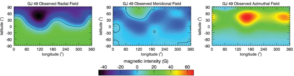
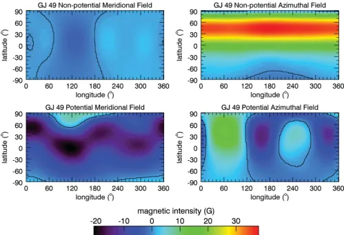
The corresponding surface magnetic maps from Donati et al. (2008) are reproduced in Figs 1 and 2. In both cases, the radial and meridional fields look very similar to a dipole, but particularly in the case of GJ 49, there is a significant azimuthal field that is unidirectional at low to mid latitudes. This is a clear signature of a non-potential field.
3 T H E S TAT I C C O R O N A L M AG N E T I C F I E L D
In order to determine the coronal structure that corresponds to these surface fields, we need to make some assumptions about the nature of the coronal field. The simplest assumption is that the field is potential, or in its lowest energy state and is determined simply by the coefficientsαlmandβlmin equations (1–3). This is the starting
point for many extrapolations of the solar magnetic field. If we wish to determine the distribution of electric currents in the corona, however, we need to allow for the non-potential components that are described by the coefficientsγlm.
3.1 Potential field extrapolation
We begin by calculating the contribution to the total field that is potential. We write Bpot in terms of a flux function such that
Bpot= −∇ and the condition that the field is potential (∇×
Bpot=0) is then satisfied automatically. The condition that the field is divergence free then reduces to Laplace’s equation∇2 =0 with solution in spherical coordinates (r,θ,φ)
=
N
l=1 l
m=−l
almrl+blmr−(l+1)Plm(θ)eimφ, (5)
where all radii are scaled to a stellar radius and the associ-ated Legendre functions are once again denoted byPlm. The two
unknowns are therefore the coefficientsalm andblm. One of these
at Library & Information Services, University of St Andrews on August 8, 2013
http://mnras.oxfordjournals.org/
Figure 2. Surface magnetic field maps of GJ 49 derived from spectropolarimetric observations (Donati et al. 2008). The single black line shows the zero-field contour that separates regions of opposite polarity.
can be determined by imposing the radial field at the surface from the Zeeman–Doppler maps. In order to determine the second un-known, we select a particular form of potential field that has the useful property that at some radius, all the field lines are open. This mimics the effect of the outward pressure of the hot coronal gas pulling open field lines to form the stellar wind. Thus, at some normalized radiusRsabove the surface (known as thesource sur-face) the field becomes radial and henceBθ(Rs)=Bφ(Rs)=0. As a result,
blm= −almR2ls+1 (6)
and we may write
Bpot r =
N
l=1 l
m=−l
BlmPlm(θ)fl(r, Rs)r−(l+2)eimφ (7)
Bpot θ = −
N
l=1 l
m=−l
BlmdPlm(θ)
dθ gl(r, Rs)r
−(l+2)eimφ (8)
Bpot φ = −
N
l=1 l
m=−l
BlmPlm(θ)
sinθ imgl(r, Rs)r
−(l+2)eimφ, (9)
where the functionsfl(r, Rs) andgl(r, Rs) which describe the in-fluence of the source surface (and hence the wind) on the magnetic field structure are given by
fl(r, Rs)=
l+1+l(r/Rs)2l+1
l+1+l(1/Rs)2l+1
(10)
gl(r, Rs)=
1−(r/Rs)2l+1
l+1+l(1/Rs)2l+1
. (11)
In the limit where the source surface is large (i.e. the magnetic field is completely closed), we recover the familiar multipolar expansions for a magnetic field. This limit corresponds toRs→ ∞and
fl(1)→1 (12)
gl(1)→l+1
1. (13)
The coefficientsBlmare determined by the surface radial field that
is derived from the Zeeman–Doppler maps [i.e. by the values ofαlm
in (1)]. This is known as thepotential field source surfacemethod. It was originally developed for extrapolating the Sun’s coronal field from solar magnetograms (Altschuler & Newkirk 1969). We use a code originally developed by van Ballegooijen, Cartledge & Priest (1998) (see also Jardine, Collier Cameron & Donati 2002).
Comparing the form of our extrapolated field given in (7–9) with the general expressions for the observed field at the surface (1–3),
we can see that our extrapolated field cannot match the observed surface field exactly. The reason is that the form of potential field we are using for the extrapolation (thepotential field source surface method) is only one type of potential field. The assumption of a source surface forces a relationship between the field components that means they are no longer independent. Whileαlmcan be simply
related toBlm, we cannot match the values ofβlmthat are derived
from the observations. Therefore, this method, which selects only one type of potential field, will not be guaranteed to reproduce the potential field contribution toBθandBφthat is fitted to the data.
With this caveat in mind, we use the observedBrat the stellar
sur-face to determineBlmand hence to obtain the potential contribution
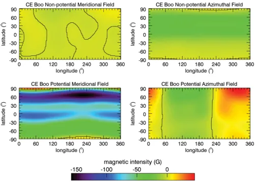
to the azimuthal and meridional fieldsBφpotandBθpot. We show these in the bottom rows of Figs 3 and 5. We note in passing that these are very similar to Figs 4 and 6 which are produced by the wind solution (see section 4). It is clear by comparison with the observed surface maps shown in Figs 1 and 2, that this potential field does not reproduce all the observed field components. In particular, the unidirectional band of azimuthal field is absent from these potential field maps. In order to extrapolate the non-potential part of the field, however, we need to make an assumption about the nature of the coronal currents. We base our extrapolation on the method devel-oped by Hussain et al. (2002). This is not a force-free solution, but it allows us to incorporate fully the non-potential contribution of the surface field and to extrapolate it into the corona.
3.2 Non-potential field extrapolation
In general, the magnetic field will be a sum of potential and non-potential terms such thatB=Bpot+Bnp. We assume that the non-potential magnetic field is perpendicular to the radial direction (i.e. it lies on spherical shells and soBnp
r =0). Furthermore, the electric currents are assumed to be derived from a potentialQ:
∇×Bnp= −∇Q. (14)
It follows that∇2Q=0, soQ(r) has a solution in terms of spherical harmonics. As shown in the Appendix, we find solutions for this non-potential magnetic field that vanish at the source surface and have the form
Bnp
r =0 (15)
Bnp θ = −
N
l=1 l
m=−l
l(l+1)ClmPlm(θ)
sinθ imhl(r, Rs)r
−(l+1)eimφ (16)
Bnp φ =
N
l=1 l
m=−l
l(l+1)ClmdPlm(θ)
dθ hl(r, Rs)r
−(l+1)eimφ, (17)
at Library & Information Services, University of St Andrews on August 8, 2013
http://mnras.oxfordjournals.org/
Figure 3. The static solution for the surface magnetic field of CE Boo, divided into its different components. The meridional component is shown in the left column and the azimuthal component in the right column. The top row shows the non-potential contribution and the bottom row the potential contribution to the total field. The single black line shows the zero-field contour which therefore separates regions of opposite polarity.
Figure 4. The wind solution for the surface magnetic field of CE Boo, divided into its meridional (left-hand column) and azimuthal (right-hand column) components. The single black line shows the zero-field contour which therefore separates regions of opposite polarity.
where
hl(r, Rs)=
1−(r/Rs)2l+1
l+(l+1)(1/Rs)2l+1
(18)
and asRs→ ∞we recoverhl(1)→1/l.
While this is not the most general form of non-potential field, it has the useful property that the equations forBpotandBnpare now structurally very similar to the forms used in (1–3) to describe the surface field. The coefficientsγlmandClmthat govern the
non-potential field components can be simply related. This allows us
at Library & Information Services, University of St Andrews on August 8, 2013
http://mnras.oxfordjournals.org/
[image:5.595.42.546.452.642.2]Figure 5. The static solution for the surface magnetic field of GJ 49, divided into its different components. The meridional component is shown in the left-hand column and the azimuthal component in the right-hand column. The top row shows the non-potential contribution and the bottom row the potential contribution to the total field. The single black line shows the zero-field contour which therefore separates regions of opposite polarity.
to match the observed non-potential component of the field exactly to our model and to extrapolate it into the corona. Thus, while the potential part of our extrapolated field will not reproduce an exact match to the potential part of the observed surface field, the non-potential part matches exactly.
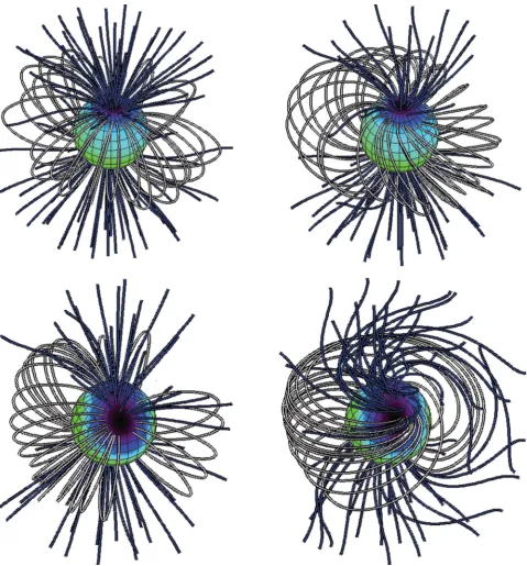
We therefore show the non-potential (top row) and potential (bot-tom row) parts of the field separately in Figs 3 and 5. The total field is the sum of both of these. Fig. 7 shows the extrapolation of this to-tal field with a source surface chosen to be at 4R. The largest closed field lines have been selected in order to highlight the structure of the large-scale field. The tilt of the dipole axis can be clearly seen in both cases, although it should be noted that the rotation axes of both stars have the same inclination to the observer’s line of sight. While the extrapolation of the potential contribution to the total field is fairly similar in both stars, the inclusion of the non-potential contribution highlights the differences between the magnetic field structures of the two stars. The non-potential component introduces an azimuthal shear into the field that is most apparent in GJ 49 (for which 52 per cent of the total magnetic energy in the surface field is non-potential).
4 T H E S T E L L A R W I N D M O D E L
To perform the stellar wind simulations, we use the three-dimensional MHD numerical codeBATS-R-USdeveloped at Univer-sity of Michigan (Powell et al. 1999).BATS-R-UShas been widely
used to simulate, e.g., the Earth’s magnetosphere (Ridley et al. 2006), the heliosphere (Roussev et al. 2003), the outer heliosphere (Linde et al. 1998; Opher et al. 2003, 2004), coronal mass ejections (Manchester et al. 2004; Lugaz, Manchester & Gombosi 2005), the magnetosphere of planets (T´oth et al. 2004; Hansen et al. 2005) and stellar winds of cool stars (Vidotto et al. 2009, 2012). It solves the ideal MHD equations, that in the conservative form are given by
∂ρ
∂t + ∇ ·(ρu)=0, (19) ∂(ρu)
∂t + ∇ ·
ρu u+
p+ B2
8π I−
B B
4π
=ρg, (20)
∂B
∂t + ∇ ·(u B−B u)=0, (21) ∂ε
∂t + ∇ ·
u
ε+p+B2
8π −
(u·B)B
4π
=ρg·u, (22)
where the eight primary variables are the mass densityρ, the plasma velocityu= {ur, uθ, uϕ}, the magnetic fieldB= {Br, Bθ, Bϕ}and the gas pressurep. The gravitational acceleration due to the star with massMand radiusRis given byg, andεis the total energy density given by
ε= ρu2
2 +
p
γ−1+
B2
8π. (23)
at Library & Information Services, University of St Andrews on August 8, 2013
http://mnras.oxfordjournals.org/
Figure 6. The wind solution for the surface magnetic field of GJ49, divided into its meridional (left-hand column) and azimuthal (right-hand column) components. The top row shows the result of assuming the observed stellar rotation period of 18.6 d, while the bottom row shows the result of assuming a stellar rotation period artificially decreased to 0.6 d. The single black line shows the zero-field contour which therefore separates regions of opposite polarity.
We consider an ideal gas, sop=nkBT, wherekBis the Boltzmann constant,Tis the temperature,n=ρ/(μmp) is the particle number density of the stellar wind,μmpis the mean mass of the particle and
γ is the polytropic index (such thatp∝ργ).
As the initial state of the simulations, we assume that the wind is thermally driven (Parker 1958). At the base of the corona (r=R), we adopt a wind coronal temperatureT0=2×10⁶K and wind number densityn0=1011cm−3. The stellar rotation periodProt,M andRare given in Table 1. With this numerical setting, the initial solution for the density, pressure (or temperature) and wind velocity profiles are fully specified.
To complete our initial numerical set up, we assume that the magnetic field is either potential everywhere (i.e.,∇×B=0) or the sum of potential plus non-potential components, as described in Sections (3.1) and (3.2). The initial solution forBis found once the distance to the source surface is assumed (set at 4Rin the initial state of our runs) and the surface magnetic field is specified: either simply the radial component (in the case of a potential field) or all three components (in the case of a total potential plus non-potential field).
Once set at the initial state of the simulation, the distribution of Bris held fixed at the surface of the star throughout the simulation
run, as are the coronal base density and thermal pressure. A zero radial gradient is set to the remaining components ofBandu=0 in the frame corotating with the star. The outer boundaries at the edges of the grid have outflow conditions, i.e., a zero gradient is set
to all the primary variables. The rotation axis of the star is aligned with thez-axis, and the star is assumed to rotate as a solid body.
Our grid is Cartesian and extends inx,yandzfrom−20 to 20R, with the star placed at the origin of the grid.BATS-R-USuses block adaptive mesh refinement, which allows for variation in numerical resolution within the computational domain. The finest resolved cells are located close to the star (forr2R), where the linear size of the cubic cell is 0.02R. The coarsest cell is about one order of magnitude larger (linear size of 0.31R) and is located at the outer edges of the grid. The total number of cells in our simulations is about 15 million.
As the simulations evolve in time, both the wind and magnetic field lines are allowed to interact with each other. The resultant so-lution, obtained self-consistently, is found when the system reaches a steady state (in the reference frame corotating with the star).
5 R E S U LT S A N D D I S C U S S I O N
We have separated the magnetic fields of CE Boo and GJ 49 into their lowest energy (potential) and stressed (non-potential) components. This has allowed us to isolate both the locations where the field is stressed above its lowest energy state and also the nature of the structures that carry these stresses. We find that the departures from a lowest energy state are apparent mainly in the azimuthal field (the meridional field contributes a negligibly small non-potential component). This appears as a clearly defined mid-latitude band of
at Library & Information Services, University of St Andrews on August 8, 2013
http://mnras.oxfordjournals.org/
Figure 7. Static field line extrapolations for CE Boo (top) and GJ 49 (bottom) for fields that are purely potential (left) and those that are the sum of potential plus non-potential (right). Closed field lines which would contain coronal gas are shown white, open field lines which would contribute to the stellar wind are shown blue.
unidirectional azimuthal field (see Figs 3 and 5). This is similar to the non-potential field of the young rapid rotator AB Dor (Hussain et al. 2002) except that it appears at lower latitudes.
By extrapolating these surface fields into the corona, we can see that the presence of the non-potential field does not change the overall topology of the coronal field, but it provides an azimuthal shear (see Fig. 7). We have also explored the nature of the winds that might be associated with these surface fields by using these extrapolated fields as an initial state for an MHD wind model. As the solution evolves towards a steady state, only the radial component
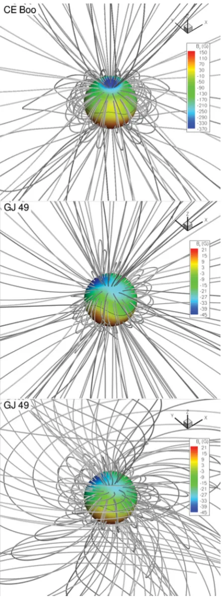
of the surface field is kept fixed – the azimuthal and meridional field components are allowed to vary in response to the available forces. The top and middle rows of Fig. 8 show the final structure of the magnetic fields of CE Boo and GJ 49. This final state was the same, regardless of whether the initial state was the total field (i.e. the potential plus non-potential field), or simply the potential field. This happens because it is the boundary conditions that will control the final state and the initial conditions of the system will be ‘flushed out’ by the wind. Therefore, we find that the mass-loss rates, angular momentum mass-loss rates, and the fluxes of surface
at Library & Information Services, University of St Andrews on August 8, 2013
http://mnras.oxfordjournals.org/
Figure 8. Final magnetic field structures for CE Boo (top row) and GJ 49 (middle row). The final state is the same, regardless of whether the initial state is the total field (i.e. the potential plus non-potential field), or simply the potential field. The bottom row shows the effect on GJ 49 of artificially decreasing the rotation period from 18.6 to 0.6 d.
field and generates an azimuthal field component, but this is fairly small at the stellar surface, particularly for such slowly rotating stars. In order to confirm the role of rotation in influencing the field structure, we also artificially increase the rotation rate of GJ 49, while keeping the initial magnetic field structure unchanged. The resulting field structure is shown in Fig. 8. While an azimuthal field develops with height in the corona, it is small at the surface and cannot explain the observations. This suggests that this azimuthal field is produced not by the wind, but by the sub-surface dynamo.
These simulations therefore suggest that the ambient winds of these slowly rotating stars are well described by the potential com-ponents of their surface fields. The strong azimuthal fields seen at the surface should not survive to the heights in the corona at which the wind is launched. They may of course be important in determin-ing flare locations and energies. For GJ 49, for example, 52 per cent of the total magnetic energy close to the surface is contained in the non-potential part of the field and is therefore available for release. It is mainly contained in a well-defined band that is centred around latitudes 30◦–40◦. This is the maximum latitude at which solar ac-tive regions are seen and from which solar coronal mass ejections are launched. This might suggest that this is the region from which flares and coronal mass ejections could be expected. On the young rapid rotator AB Dor, by comparison, (Prot =0.514 d) the band of non-potential field is strongest around 70◦–80◦(Hussain et al. 2002) which may suggest a different pattern of coronal mass ejec-tion. Such coronal mass ejections would temporarily increase the mass loading of the stellar wind and also its ram pressure, which is responsible for compressing the magnetospheres of any orbit-ing planets. Whether coronal mass ejections provide a significant contribution to either angular momentum loss or the impact of the wind on orbiting planets depends on their size and frequency. The background stellar wind that we find however is independent of the strong non-potential component of the surface fields and is primarily governed by their radial component.
AC K N OW L E D G E M E N T S
The authors acknowledge support from STFC. AAV acknowledges support from the Royal Astronomical Society. JM acknowledges support from a fellowship of the Alexander von Humboldt founda-tion.
R E F E R E N C E S
Aarnio A. N., Stassun K. G., Hughes W. J., McGregor S. L., 2011a, Sol. Phys., 268, 195
Aarnio A. N., Stassun K. G., Matt S. P., Hughes W. J., McGregor S. L., 2011b, in Johns-Krull C., Browning M. K., West A. A., eds, ASP Conf. Ser. Vol. 448, 16th Cambridge Workshop on Cool Stars, Stellar Systems and the Sun. Astron. Soc. Pac., San Francisco, p. 43
Altschuler M. D., Newkirk G. Jr, 1969, Sol. Phys., 9, 131
at Library & Information Services, University of St Andrews on August 8, 2013
http://mnras.oxfordjournals.org/
Barnes J., Collier Cameron A., James D. J., Donati J.-F., 2000, MNRAS, 314, 162
Barnes J. R., Collier Cameron A., Donati J.-F., James D. J., Marsden S. C., Petit P., 2005, MNRAS, 357, L1
Brickhouse N., Dupree A., 1998, ApJ, 502, 918 Byrne P., Eibe M., Rolleston W., 1996, A&A, 311, 651 Collier Cameron A., Robinson R. D., 1989a, MNRAS, 238, 657 Collier Cameron A., Robinson R. D., 1989b, MNRAS, 236, 57 Collier Cameron A., Woods J. A., 1992, MNRAS, 258, 360 Donati J.-F., Brown S., 1997, A&A, 326, 1135
Donati J.-F., Collier Cameron A., 1997, MNRAS, 291, 1
Donati J.-F., Mengel M., Carter B., Cameron A., Wichmann R., 2000, MN-RAS, 316, 699
Donati J.-F. et al., 2006, MNRAS, 370, 629 Donati J. et al., 2008, MNRAS, 390, 545
Dupree A., Brickhouse N., Doschek G., Green J., Raymond J., 1993, ApJ, 418, L41
Eibe M. T., 1998, A&A, 337, 757 G¨udel M., 2004, A&AR, 12, 71
G¨udel M. et al., 2001, in Giaconni R. L., Serio S., Stella S. S., eds, ASP Conf. Ser. Vol. 234, Proceedings of ‘X-ray astronomy 2000’. Astron. Soc. Pac., San Francisco, p. 73
Hansen K. C., Ridley A. J., Hospodarsky G. B., Achilleos N., Dougherty M. K., Gombosi T. I., T´oth G., 2005, Geophys. Res. Lett., 32, 20 Hussain G. A. J., van Ballegooijen A. A., Jardine M., Collier Cameron A.,
2002, ApJ, 575, 1078
Jardine M., van Ballegooijen A. A., 2005, MNRAS, 361, 1173 Jardine M., Collier Cameron A., Donati J.-F., 2002, MNRAS, 333, 339 Jeffries R., 1993, MNRAS, 262, 369
Jeffers S. V., Donati J.-F., Alecian E., Marsden S. C., 2011, MNRAS, 411, 1301
Khodachenko M. L. et al., 2007, Astrobiology, 7, 167
Linde T. J., Gombosi T. I., Roe P. L., Powell K. G., Dezeeuw D. L., 1998, J. Geophys. Res., 103, 1889
Lugaz N., Manchester W. B., IV, Gombosi T. I., 2005, ApJ, 627, 1019 Maggio A., Pallavicini R., Reale F., Tagliaferri G., 2000, A&A, 356, 627 Manchester W. B., Gombosi T. I., Roussev I., De Zeeuw D. L., Sokolov I.
V., Powell K. G., T´oth G., Opher M., 2004, J. Geophys. Res., 109, 1102 Marsden S. C., Waite I. A., Carter B. D., Donati J.-F., 2005, MNRAS, 359,
711
Marsden S. C., Donati J.-F., Semel M., Petit P., Carter B. D., 2006, MNRAS, 370, 468
Mestel L., 1999, Stellar Magnetism. Oxford Univ. Press, Oxford Morin J., 2012, in Reyl´e C., Charbonnel C., Schultheis M., eds, EAS
Publications Series. Vol. 57, Magnetic Fields from Low-Mass Stars to Brown Dwarfs. EDP Sciences, France, p. 165
Morin J. et al., 2008, MNRAS, 390, 567
Morin J., Donati J.-F., Petit P., Delfosse X., Forveille T., Jardine M. M., 2010, MNRAS, 407, 2269
Opher M., Liewer P. C., Gombosi T. I., Manchester W., DeZeeuw D. L., Sokolov I., Toth G., 2003, ApJ, 591, L61
Opher M. et al., 2004, ApJ, 611, 575 Parker E. N., 1958, ApJ, 128, 664 Petit P. et al., 2008, MNRAS, 388, 80
Pinto R. F., Brun A. S., Jouve L., Grappin R., 2011, ApJ, 737, 72 Pointer G. R., Jardine M., Collier Cameron A., Donati J.-F., 2002, MNRAS,
330, 160
Powell K. G., Roe P. L., Linde T. J., Gombosi T. I., de Zeeuw D. L., 1999, J. Comput. Phys., 154, 284
Ridley A. J., de Zeeuw D. L., Manchester W. B., Hansen K. C., 2006, Adv. Space Res., 38, 263
Riley P., Linker J. A., Miki´c Z., Lionello R., Ledvina S. A., Luhmann J. G., 2006, ApJ, 653, 1510
Roussev I. I., Gombosi T. I., Sokolov I. V., Velli M., Manchester W., IV, DeZeeuw D. L., Liewer P., T´oth G., Luhmann J., 2003, ApJ, 595, L57 Sanz-Forcada J., Maggio A., Micela G., 2003, A&A, 408, 1087 Schatten K., Wilcox J., Ness N., 1969, Sol. Phys., 6, 442
Schrijver C., Mewe R., van den Oord G., Kaastra J., 1995, A&A, 302, 438
Strassmeier K. G., 2009, A&AR, 17, 251
T´oth G., Kov´acs D., Hansen K. C., Gombosi T. I., 2004, J. Geophys. Res., 109, 11210
van Ballegooijen A., Cartledge N., Priest E., 1998, ApJ, 501, 866 Vidotto A. A., Fares R., Jardine M., Donati J.-F., Opher M., Moutou C.,
Catala C., Gombosi T. I., 2012, MNRAS, 423, 3285
Vidotto A. A., Opher M., Jatenco-Pereira V., Gombosi T. I., 2009, ApJ, 703, 1734
Wang Y.-M., Sheeley N. R. Jr, Rouillard A. P., 2006, ApJ, 644, 638 Weber E., Davies L., 1967, ApJ, 148, 217
A P P E N D I X A : T H E N O N - P OT E N T I A L F I E L D
We look for solutions for the non-potential field that are of the form
Bnp,r=0, Bnp,θ = r 1 sinθ
∂F
∂φ, Bnp,φ= −
1
r ∂F
∂θ, (A1)
whereF(r) is a scalar function. These automatically satisfy∇ ·B= 0. Furthermore, the electric currents are assumed to be derived from a potentialQ:
∇ ×Bnp= −∇Q. (A2)
It follows that∇2Q=0, soQ(r) has a solution in terms of spherical harmonics. Inserting equation (A1) into (A2), we find from the radial component:
−r12
1 sinθ ∂ ∂θ sinθ∂F
∂θ +
1 sin2θ
∂2F
∂φ2
= −∂∂Qr , (A3)
and from theθandφcomponents:
1 r ∂ ∂r ∂F
∂θ = −
1
r ∂Q
∂θand
1 r ∂ ∂r 1 sinθ ∂F
∂φ = −
1
rsinθ
∂Q ∂φ,
(A4)
which can be integrated with respect toθandφ:
∂F
∂r = −Q. (A5)
We now introduce a third scalarC(r) such that
F=r2∂C
∂r, (A6)
then equation (A5) yields
Q= −∂
∂r
r2∂C
∂r . (A7)
Inserting these expressions for F and Q into equation (A3) we obtain
∂ ∂r(r
2∇2C
)=0. (A8)
Assuming∇2C=0 at the stellar surface, it follows that this condi-tion is true at all heights, soC(r) is also a harmonic function. We now writeCas a sum over spherical harmonics:
C(r, θ, φ)= lm
Clmql(r)Plm(θ)eimφ, (A9)
wherelis the harmonic degree (l=1, 2, . . . ),mis the azimuthal mode number (−l≤m≤ +l),Plm(θ) is the associate Legendre
function, andql(r) describes the radial dependence of the various
modes. Note that the functionql(r) defined here is different from
the functionfl(r) for the potential field (see Hussain et al. 2002).
at Library & Information Services, University of St Andrews on August 8, 2013
http://mnras.oxfordjournals.org/
the stellar surface (r = 1). Secondly, since C(r) is a harmonic This paper has been typeset from a TEX/LTEX file prepared by the author.
at Library & Information Services, University of St Andrews on August 8, 2013
http://mnras.oxfordjournals.org/