Cancer profiles by Affinity Propagation

Cancer profiles by Affinity Propagation

D. Soria

, F. Ambrogi

, E. Raimondi

, P. Boracchi

, J.M. Garibaldi

, E. Biganzoli

_{School of Computer Science, University of Nottingham, UK}

2

_{Istituto di Statistica Medica e Biometria “G.A. Maccacaro”, Universit`a degli Studi di Milano, Milano, Italy}

3

_{Struttura di Statistica e Biometria, Fondazione IRCCS Istituto Nazionale Tumori, Milano, Italy}

Abstract

The Affinity Propagation algorithm is applied to various problems of breast and cutaneous tumours subtyping using traditional biologic markers. The algorithm provides a pro-cedure to determine the number of profiles to be considered. Well know breast cancer case series and cutaneous melanoma were used to compare the results of the Affinity Propagation with the results obtained with standard algo-rithms and indexes for the optimal choice of the number of clusters.

Results from Affinity Propagation are consistent with the results already obtained having the advantage of providing an indication about the number of clusters.

1

Introduction

Genomic analysis renewed interest in clustering tech-niques. After the seminal paper of Eisen and colleagues [6], proposing hierarchical clustering and the visual inspection of the dendrogram to discover unknown pattern of gene as-sociations, the use of clustering has become more and more popular especially for discovering profiles in cancer with respect to high-throughput genomic data. Important appli-cations of the Eisen method are the work of Bittner [3] on clustering of cutaneous melanoma and the works of van’t Veer [25] and Perou [19] on breast cancer.

Recently a classification of breast carcinoma using tra-ditional tumor markers was proposed [1]. The classifica-tion was in agreement with the classificaclassifica-tions obtained with c-DNA microarray data [19, 25]. Different clustering al-gorithms were used to choose a stable solution across dif-ferent clustering methods. At last a classification in four clusters was preferred and suggested a possible separation of high risk profiles. One of the main problems connected with cluster analysis is the choice of the number of clusters. In classical cluster analysis it is customary to use indexes to compare one cluster solutions to other cluster solutions and to choose the one suggested as optimal.

In the previous application [1], different indexes were used to select an optimal partition. Namely the indexes pro-posed by Calinski and Harabasz [4], Krzanowski and Lai [14], Hartigan [12] and Tibshirani et al. [23], were con-sidered. It is worth noting that the visual inspection of the dendrogram suggested by Eisen [6] is an informal method to determine the number of clusters. Such a procedure was criticized in [10] as it can cause difficulty in assessing the validity of the grouping.

According to Getz [9], the number of clusters should be determined internally by the clustering algorithm and should not be externally prescribed.

In this work a new clustering algorithm, the Affinity Propagation [8], will be adopted to cluster cancer patients in order to evaluate its performance with respect to the tra-ditional applications. Several datasets, already published in literature, were considered in our study: the melanoma data of Bittner et al. [3], and four different breast cancer data analyses: namely, the studies of Ambrogi et al. [1], Perou et al. [19], van’t Veer et al. [25], and Sotiriou et al. [22]. Although this algorithm does not determine automatically the number of clusters it provides a consistent method to suggest the number of clusters to be created which can be useful to detect different levels of association pattern.

2

Material and methods

2.1

Case data

This section includes a description of the case series adopted in the work.

The information on 633 patients operated on for primary infiltrating breast cancer between 1983 and 1992, archived at the Pathology department of the University of Ferrara, was retrospectively analyzed in the work of Ambrogi et al. [1].

progesterone receptors status (PR), Ki-67/MIB-1 prolifera-tion index (Ki-67), c-ErbB-2/NEU (NEU) and the p53 on-cosuppressor gene (p53).

Values of ER, PR and NEU tended to be grouped on the following values: 0%, 10%, 25%, 50%, 75% and 100%; they were consequently discretized on those values. Values of Ki-67 and p53 were used as originally measured.

A second dataset was also analyzed: the melanoma data of Bittner et al. [3]. These data consist of gene expression profiles obtained on a collection of 38 samples, comprised of 31 melanoma tumors and 7 controls. For the analysis de-scribed in Section 3, the data from the seven control speci-mens were excluded and only the ratios for the 3613 genes that were considered “well measured” (that is their inten-sities were sufficiently high) were used. These ratios were converted to log2 ratios.

Another dataset on breast cancer that was considered for investigation was the one of Perou et al. [19]. Variation in gene expression patterns in a set of 65 surgical speci-mens of human breast tumours from 42 different individ-uals have been characterized, using complementary DNA representing 8102 human genes. According to the authors, these patterns provided a distinctive molecular portrait of each tumour [19]. Sets of co-expressed genes were identi-fied for which variation in messenger RNA levels could be related to specific features of physiological variation. The tumours could be classified into subtypes distinguished by differences in their gene expression patterns. In their paper, Perou et al. focused on a set of 1,753 genes in 65 experi-mental tissue samples. In each sample, the ratio of the abun-dance of transcripts of each gene to its median abunabun-dance across all tissue samples, is reported.

Data and original analyses of Bittner and Perou are fully described in the book “Design and Analysis of DNA Mi-croarray Investigations” by Simon and colleagues [21].

The dataset analysed in van’t Veer et al. [25] was also considered in this study: they used DNA microarray anal-ysis on primary breast tumours of 117 young patients, and applied supervised classification to identify a gene expres-sion signature strongly predictive of a short interval to dis-tant metastases in patients without tumour cells in local lymph nodes at diagnosis. All patients were lymph node negative and under 55 years of age at diagnosis. Unsuper-vised clustering detected two subgroups of breast cancer, which differ in ER status and lymphocytic infiltration.

The last dataset we analysed was taken from Sotiriou et al. [22] where tumour samples from 99 patients with primary local breast cancer were accessed from the John Radcliffe Hospital from January 1993 to December 1994. All of the tumor samples were invasive ductal carcinomas; 46 individuals were node negative and 53 were node pos-itive. Almost all of the patients received adjuvant treat-ment after surgery, consisting of radiotherapy (80 patients),

chemotherapy (32 patients), and endocrine therapy (78 pa-tients) according to accepted practice guidelines at that time. From each woman belonging to the cohort, a tumour tissue sample, on which all the analyses were run, was ex-tracted using microarray technology. For each spot, Log (base 2) ratios between red signal and green signal were cal-culated. The log ratios were then normalized within each array by subtracting from each the median log ratio value across the spots on the array.

2.2

Statistical Methods

The clustering technique Affinity Propagation (AP, [8]) will be adopted for grouping tumours with similar biologi-cal characteristics.

As other clustering algorithms, this method uses data to find a set of centers such that the sum of squared errors be-tween data points and their nearest center is small.

Like other traditional clustering techniques, the Affinity Propagation algorithm determines the centers from real data points (exemplars). These exemplars correspond, for exam-ple, to the medoids in the algorithm Pam [13] (Partitioning Around Medoids, a more robust version of K-means), that is k representative objects among the observations of the dataset that should represent the structure of the data.

As a technical detail, it is worth noting that K-means al-gorithm does not use exemplars, as the centers are not gen-erally actual data points.

Affinity Propagation combines the properties of different classes of clustering algorithms. On one hand, algorithms like hierarchical clustering are based on grouping pairs of objects with high Affinity. On the other hand model-based clustering uses a probability model based on a mixture of class conditional distributions. Affinity Propagation uses both pairs comparison and a probability model to determine the optimal grouping. According to a more technical point of view, Affinity Propagation can be derived as the sum-product algorithm in a graphical model describing the mix-ture model [7].

The first step for the algorithm implementation is to choose a measure of similarity, s(i,k), between all pairs of data points. In AP terminology, s(i,k) quantifies how well the data point with index k is suited to be the exemplar for data point i. Generally, as similarity, it is used the negative Euclidean distance. In the case of c-DNA data the Pearson correlation is generally used as similarity measure [3].

This method does not require the number of clusters to be prespecified.

k

i

points with larger values of s(i,i) are more likely to be cho-sen as exemplars. At the beginning, the AP simultaneously considers all data points as potential exemplars (Input the preferences common for all data points).

The number of identified exemplars is influenced by the values of the input preferences, but also emerges as a result of the message passing structure that is illustrated subse-quently. For very small value of input s(i,i), for every i, all data points are grouped in one large cluster with a single ex-emplar; in the opposite case of large s(i,i) for every i, each data point prefers to be its own exemplar. In general, the initial value of the preferences is set equal to the median of all input similarities (resulting in a moderate number of clusters) or to their minimum (resulting in a small number of clusters).

The AP is a method that recursively transmits messages (that will be defined subsequently) between pairs of data points until a good set of exemplars and corresponding clus-ters emerges.

The algorithm is named Affinity Propagation because at any point in time, each message reflects the current Affinity between one data point and the other that is its exemplars.

In practice, it is adopted a message-passing algorithm in which each data point i furnishes a measure to suggest another data point k to be selected as cluster center, taking into account other potential exemplars for point i.

There are two kinds of message being passed between each pairs of data points that represent the relationship be-tween data points:

• “responsibility”: sent from data point i to candidate exemplar k. It is a measure that quantifies how well-suited point k is to be the exemplar for point i, taking into account other potential exemplars for point i. This message is represented by r(i,k) and it is computed us-ing this formula:

r(i, k) =s(i, k)− max

k0_s.t.k0_6=k{a(i, k

0_{) +s(i, k}0_)}

where s.t. means “so that”;

• “availability”: sent from candidate exemplar point k to point i. It is a measure that reflects the evidence for point i to choose point k as its exemplar, considered that other points may have k as an exemplar. This mes-sage is represented by a(i,k) and it is computed using

this formula:

a(i, k) = min{0, r(k, k)+ X

i0_s.t.i0_{∈{/ i,k}}

max{0, r(i0, k)}}

A particular measure is the “self-responsibility”, that is r(k,k); it reflects accumulated evidence that point k is an exemplar and how it would be unsuitable to be integrated in a group of another cluster center.

At the beginning of the algorithm, the availabilities are initialized to zero, so r(i,k) is set to the input similarity be-tween point i and its potential exemplar k minus the largest of the similarities between point i and other candidate ex-emplars. After the computation of all the responsibilities, the availabilities are worked out using the previous formula. Only the positive portions of responsibilities between the candidate exemplar k and other data points i’ are added be-cause it is only necessary for a good exemplar to explain some data points well ( r(i0_{, k) > 0 ) regardless of how}

poorly it explains other data points (r(i0_{, k)<0). In fact,}

ifr(i0, k)<0, k is not suited to be the exemplar for point i’. So in this case, the point i’ will not contribute to the message passing from candidate exemplar k to point i.

After that, the messages are recursively updated for a fixed number of iterations or until a stable clustering result. At any stage, the availabilities and responsibilities can be combined to identify exemplars. For point i, the value k that maximizesa(i, k) +r(i, k)identifies point i as exem-plar if k=i or identifies the data point that is the exemexem-plars for point i. In other words, as suggested in [5], after ex-changing messages, Affinity Propagation identifies a set of exemplarsKso as to maximize the net similarity, which is defined by the authors as

X

i /∈K

max

k∈Ks(i, k) +

X

k∈K

p(k)

wherep(k)is the a priori preference that pointkbe chosen as an exemplar.

At the end of the message passing, we obtain the number of clusters and the labels for each data point of its exem-plars.

All the equations shown above are derived and explained in details in the Supporting Online Material for [8].

Given the initial common preference AP defines a unique solution. One of the strong points of AP is its computational efficiency, as described in [17]. The algorithm is feasible even in presence of very large data sets.

In all our applications of AP,1−P earson correlation was used as similarity. The only exception was in the first case series where the negative Euclidean distance was used. These choice were in accordance with the ones adopted by the authors of the works considered.

Multiple correspondence analysis (MCA), see Greenacre [11] or Lebart et al. [16], was used as visualization tech-nique to study the composition of the clusters for the breast cancer data due to the discretization of the values of the biomarkers. The five biologic markers (ER, PgR, Ki-67, NEU and p53) were used to create the MCA plot (active in-formation). The cluster classifications were used as passive information. The amount of information explained by the first two axes was calculated following the approach sug-gested by Benzecr´ı [2]. In fact, due to a geometric property of MCA, the percentages of the inertia explained by each axis are always a pessimistic indicator of the quality of the representation. Therefore, Benzecr´ı suggested the follow-ing indicator:

ϕ(λ) =

_p

p−1

2

λ−1 p

2

where p is the number of variables andλis the principal inertia. For the melanoma data principal component plots [26] were used to visualize the separation of the tumor sam-ples according to the c-DNA microarray data.

3

Results

3.1

Ambrogi et al. breast cancer biomarkers data

AP was applied to the breast cancer data analyzed in [1] where the final clustering was obtained using a K-Medoids algorithm to generate four clusters.

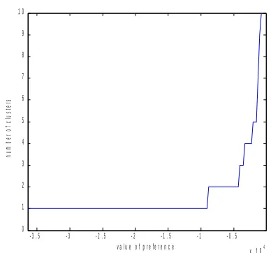
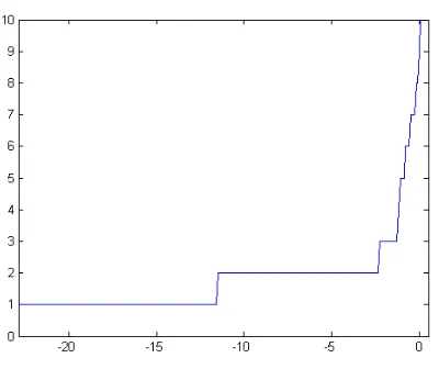
A graphical evaluation of the effect of the value of the input preference on the number of clusters for the breast cancer data is reported in Fig. 1.

The presence of three main plateaus in correspondence with two, four and five clusters is shown.

When doing the analysis with two clusters (results not shown), by using an input preference value in correspon-dence with that plateau, results consistent with expectations tied to data from literature were obtained. Indeed, one clus-ter was associated with null values of ER and PR, the other with high values of these biological markers.

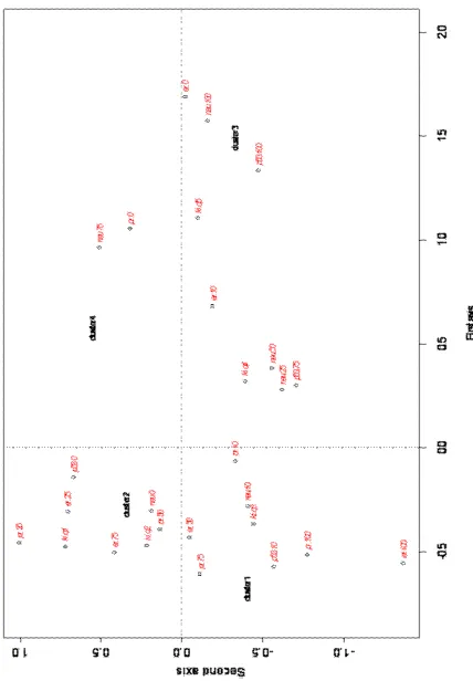
Then the message-passing algorithm was run with an in-put preference to obtain 4 clusters. The results are reported in the Multiple correspondence analysis plot (Fig. 2). The

- 3 . 5 - 3 - 2 . 5 - 2 - 1 . 5 - 1 - 0 . 5

x 1 04 0

1 2 3 4 5 6 7 8 9 1 0

v a l u e o f p r e f e r e n c e

n

u

m

b

e

r

o

f

c

lu

s

te

rs

Figure 1. The effect of the value of the input preference on the number of clusters for the Ambrogi et al. data

information explained by the first two axes is near to 89%. Therefore, the two-dimensional plots are expected to be ef-fective representations of the associations displayed.

The MCA plot was generated with the categories of the five biological markers as active information and the AP cluster classification as passive.

As for the contribution of the categories of the biological markers to the construction of the MCA axes, along the first axis there was a separation between high values of PR, ER and the categories of ER and PR absent, high NEU, p53 and Ki-67. The second MCA axis mainly separated the highest values of ER and PR from low PR, Ki-67 and null category of p53.

Null values of PR and high values of NEU were asso-ciated with the Cluster 4. Null values of ER, highest val-ues of p53, Neu and Ki-67 were associated with Cluster 3. Therefore, Cluster 3 and Cluster 4 represent groups that are associated with characteristics known to be poor prognos-tic factors. Whereas, Cluster 1 was associated with highest values of ER and PR, so it seemed to represent subject with characteristics known to be good prognostic factors. Clus-ter 2 seemed to be associated with inClus-termediated values of PR and ER and null values of Neu; so also this cluster was associated with less aggressive tumour features. As for the triple negative patients, null values of PR, ER and NEU as-sociated with positive values of p53 were grouped in Cluster 3.

us-Figure 2. MCA plot of the five discretised bio-logical markers ER, PR, MIB, NEU, p53 (active information) and four clusters (passive infor-mation)

AP CLUSTERS

PREVIOUS WORK’S CLUSTERS

1 2 3 4

1 253 1 0 2

2 1 122 0 84

3 0 1 88 2

4 1 25 1 52

Table 1. The distribution of subjects between new and old classification (Ambrogi et al. data)

ing K-Medoids and the classification using AP is reported in Table 1.

If these results were compared with those of the previous work, null values of PR, ER, NEU and p53 were grouped in Cluster 2, which was the cluster most similar to the charac-teristics of total sample. Instead, in this new classification null values of PR, ER and NEU associated with null val-ues of p53 lay in Cluster 4, a cluster that is not similar to total sample for the distribution of biological markers and represents groups with poor prognostic factors.

Afterwards, the AP algorithm was applied again to ob-tain a division of subjects in 5 groups and to compare these results with the four clusters. To do this, a preference value from the plateau in correspondence of five clusters in the first graphic was chosen.

The distribution of subjects between the classification using K-Medoids and the classification using AP is reported in Table 2.

Cluster 4 was more associated with PR absent and high values of NEU. Cluster 2 seemed to be more associated with intermediated values of PR and ER and null values of Neu; it was more associated also with low values of KI-67.

As before Cluster 1 and Cluster 2 were associated with less aggressive tumour features, whereas Cluster 3 and Cluster 4 represents groups with a negative prognosis.

Cluster 5 was mainly characterized by PR absent and high value of NEU. Null values of PR, ER ad NEU asso-ciated with positive values of p53 were grouped in Cluster 3. Unlike the previous classification, when we divided sub-jects in five groups null values of PR, ER and NEU associ-ated with null values of p53 move from Cluster 4 to Cluster 5.

3.2

Bittner et al. melanoma data

AP CLUSTERS

PREVIOUS WORK’S CLUSTERS

1 2 3 4 5

1 211 40 0 1 4

2 0 123 0 0 84

3 0 1 87 0 3

4 1 2 0 74 2

Table 2. The distribution of subjects between new and old classification (Ambrogi et al. data)

0.

0

0.

2

0.

4

0.

6

0.

8

1 _{13 14 15 16 17 19 18 21 23 22 25 20 24 26 29 31 30 27 28} 3 5 4 8 6 7 _{11 10} 2 ₁₂ 9

Figure 3. Dendrogram resulting from the ap-plication of hierarchical algorithm to Bittner et al. dataset

and by cutting the dendrogram by visual inspection [10].

In Fig. 3 the dendrogram resulting from the application of a hierarchical algorithm with average linkage and a sim-ilarity matrix based on Pearson correlation is reported. The two clusters were obtained by cutting the tree to obtain 5 clusters. In this way the 31 melanomas were divided in a single group comprising 20 melanomas while the remain-ing 11 (actually grouped in 4 clusters) were considered to-gether.

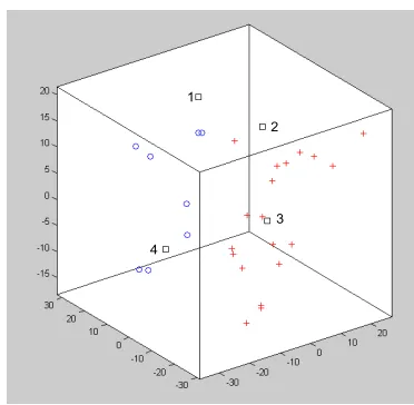
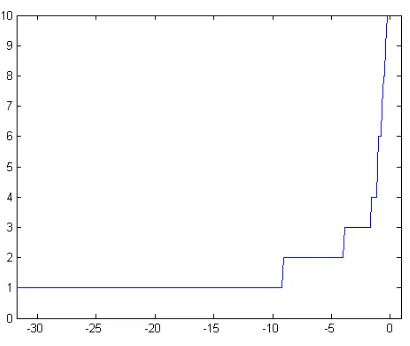
AP algorithm was applied to the melanoma data using a distance matrix based on correlations. The resulting plot of the cluster number for different preferences levels is re-ported in Fig. 4. The plot suggests solutions with 2, 3 and 5 clusters. The solution with 5 clusters is the one more sim-ilar to the one obtained by Bittner and colleagues. The 3-dimensional principal component plot in Fig. 5 shows the two groups of the 31 melanomas. The red crosses corre-spond to the “interesting” cluster identified by Bittner and colleagues. The four black squares are tumors classified differently by AP and the hierarchical algorithm. The con-cordance between the two methods appears satisfying.

- 4 - 3 . 5 - 3 - 2 . 5 - 2 - 1 . 5 - 1 - 0 . 5 0 0 . 5 1 0

5 1 0 1 5 2 0 2 5 3 0

Figure 4. The effect of the value of input preference on the number of clusters for the melanoma data

1

2

3 4

1

2

3 4

Figure 6. The effect of the value of input preference on the number of clusters for the Perou et al. data

3.3

Perou et al. breast cancer data

In the work of Perou and colleagues [19], an average-linkage hierarchical clustering method, as implemented by [6], was used to group the experimental samples on the basis of similarity in their patterns of expression. In the dendrogram derived from the hierarchical clustering, two large branches were apparent separating the tumour sam-ples into those that were clinically described as ER posi-tive and those that were ER negaposi-tive. Within these large branches there were smaller branches for which common biological themes could be inferred, namely basal-like, Erb-B2+, normal-like and luminal epithelial/ER+ cancers.

As done in Lama et al. [15], missing values were im-puted with the average values of neighbor genes resulted from a k Nearest Neighbors (k-NN) algorithm, setting k=10 (R software packageEMV, see [24]). The 10 genes ‘more similar’ to the one with missing value were selected on the basis of the sample correlation: a measure which conforms well to the intuitive biological meaning of ‘co-expression’. In this way, all the unavailable data could be recovered and a 1753 x 65 matrix obtained, where rows represented genes and columns represented samples.

The AP algorithm was run and the effect of the value of input preference against the number of clusters is visible in Fig. 6.

By the inspection of plateaus, two, three, four and six may be considered as numbers of clusters determining sta-ble solutions.

When considering two clusters a clear correspondence with the ER+ and ER- groups was not evident. In particular

AP CLUSTERS PREVIOUS

WORK’S CLUSTERS

1 2

ER pos 26 22

ER neg 8 4

Table 3. The distribution of subjects between new and old classification (Perou et al. data)

AP CLUSTERS

PREVIOUS WORK’S CLUSTERS

1 2 3 4

Basal 8 0 0 0

Erb-B2 3 2 1 1

Normal 0 11 0 0 Luminal 7 3 16 10

Table 4. The distribution of subjects between new and old classification (Perou et al. data)

the distribution shown in Table 3 was obtained (please note that for 5 patients information about their ER status was missing):

Considering three clusters, the ER- group was basically identified by the first cluster, which, on the other hand, con-tained also several ER+ patients (table not shown).

For four clusters a comparison with the four groups de-termined by the authors was done: from Table 4 it can be seen that all the basal-like tumours were captured by Clus-ter 1 and the normal-like tumours were assigned to ClusClus-ter 2. Clusters 3 and 4 seem to be characterised by the lumi-nal/epithelial cancers. Instead, the Erb-B2 group was not captured by a single cluster by the AP. It is important to note that in their work, Perou and colleagues assigned three samples to the ER negative group without specifying which of the four subgroups they are part of.

Finally, when our database was divided in six clusters it was found what is reported in Table 5.

Also with this classification in six groups, the Basal-like patients were assigned to Cluster 1. Instead the Normal ones were divided in Clusters 2 and 5. Clusters 3, 4 and 6 seemed to be three Luminal groups. Moreover, the

Erb-AP CLUSTERS

PREVIOUS WORK’S CLUSTERS

1 2 3 4 5 6

Basal 7 0 0 0 1 0

Erb-B2 2 2 0 1 0 2

Normal 0 5 0 0 6 0

Luminal 2 2 15 10 1 6

Figure 7. The effect of the value of input pref-erence on the number of clusters for the van’t Veer et al. data

B2 group was not captured by a single cluster by the AP.

3.4

van’t Veer et al. breast cancer data

In the work of van’t Veer et al. [25], an unsupervised hi-erarchical clustering algorithm allow the authors to cluster 117 tumours on the basis of thousands of genes. For clus-tering, the ‘one minus correlation’ distance was used by the authors as described in the Supplementary Information for [25]. In this way two subgroups of breast cancer were de-tected, differing in ER status (ER-positive and ER-negative) and lymphocytic infiltration (see Fig. 1a in [25]).

293 genes had missing information for all 117 patients. These genes were excluded for the analysis. Other missing values were detected in the remaining data and, ss done for the Perou data, they were imputed with k-NN algorithm. In this way, our data matrix had 117 tumours and 24188 genes of log ratio of the intensities of the red and green channels. Over this dataset, Affinity Propagation algorithm was ap-plied in order to verify the two ER groups, obtaining the plot in Fig. 7 showing the effect of the value of the common input preference on the number of clusters.

From the plot above, looking at the plateaus, solutions with two, three, five, six and seven clusters were suggested. It is worth noting that AP was not able to indicate a solu-tion with four clusters but one in six groups was evident in accordance with results previously obtained by Perou et al. [19].

When considering two clusters a very good concordance with the two groups obtained separating the ER positive and ER negative patients could be seen. In fact, just 16 over 117 cases did not show such a correspondence (see Table 6).

AP CLUSTERS PREVIOUS

WORK’S CLUSTERS

1 2

ER pos 64 11

ER neg 5 37

Table 6. The distribution of subjects between new and old classification (van’t Veer et al. data)

The split in three clusters is nothing more than a subdi-vision of the previously determined Cluster 1 into two sub-groups (table not shown).

3.5

Sotiriou et al. breast cancer data

Cluster analyses were conducted to search for natural groupings in the profiles. As in the original analysis of Sotiriou and colleagues, before clustering, a screening pro-cedure was applied to eliminate genes showing minimal variation across the set of 99 specimens. Specifically, for each gene, the 5th and 95th percentiles of the ratios were calculated. If the ratio of the 95th to 5th percentile was<3 that gene was not included in the cluster analysis. This pro-cess left 706 probe elements for the cluster analysis [22].

Authors applied hierarchical agglomerative clustering to these normalized log ratios by using both compact link-age and averlink-age linklink-age and both Euclidean and one minus Pearson correlation distance metrics. Normalized log ratios were median-centered within each gene for all of the cluster analyses. The clustering results obtained by using compact linkage with one minus Pearson correlation distance applied to the 706 probe elements appeared by visual inspection to yield the most distinctive clusters (remaining blinded to any clinical or outcome variables), and hence this was the clus-tering algorithm used for the unsupervised cluster analyses based on these probe elements.

Hierarchical clustering results showed that the tumor samples could be confidently separated into two main groups primarily associated with ER status as determined by the ligand-binding assay and confirmed by immunohis-tochemistry. Eighty-two percent of the tumors in the left main branch are ER-, and 88% of the tumors in the right main branch are ER+ by immunohistochemistry. This find-ing corroborated the earlier analysis that the major factor discriminating the expression phenotype is ER status. As expected, the ER- cluster had a higher percentage of high-grade tumors than the ER+ cluster. The dendrogram further branched into smaller subgroups within the ER+ and ER-classes.

Figure 8. The effect of the value of input preference on the number of clusters for the Sotiriou et al. data

it was possible to distinguish the “basal 1” group from the “basal 2” one. Moreover, in the ER- group, a subgroup char-acterised by the over-expression of the HER2/NEU oncogen was evident in the basal subgroup.

Concerning the ER positive group, subjects in this co-hort were characterised by the expressions of genes specific of the “luminal-like” tumours. This group was further seg-regated into three smaller subclasses: luminals 1, 2, and 3.

When considering this dataset for the AP analysis, the same technique previously described for dealing with miss-ing values was used.

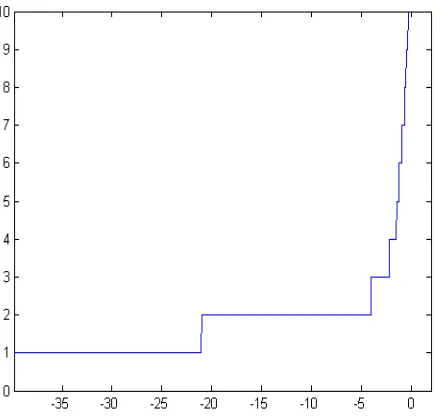
As for the other datasets considered, the effect of the value of input preference on the number of clusters is re-ported in Fig. 8.

As it can be seen from the plot, there are three main plateaus in correspondence of solutions with two, three and four clusters and other two smaller ones suggesting six and seven groups. When considering two groups, results con-sistent with the ones from literature and the two groups of Sotiriou et al. are derived. In fact, classification of sub-jects affected by breast cancer is associated to the ER sta-tus: basing on the immunohistochemistry, the first cluster is characterised by 64% of ER negative, while the second by the 92% of ER positive patients (see Table 7). The dis-tribution of subjects in the two clusters with respect to the histological grade is also reported in Table 7.

From the table above it can be seen that the ER- group (Cluster 1) is basically formed by those patients with histo-logical grade equal to two or three.

AP CLUSTERS

1 2

PREVIOUS WORK’S CLUSTERS

Grade 1 2 14

Grade 2 14 24 Grade 3 31 14

ER pos 17 48

ER neg 30 4

Table 7. The distribution of subjects between AP clusters, grade, and ER status (Sotiriou et al. data)

After that, in order to obtain a classification of 99 pa-tients in three groups, a preference value in correspondence of the proper plateau was chosen. With this value as an in-put, the Affinity Propagation algorithm was run again. From the classification in three clusters, a particular group, Clus-ter 3, is visible: it is mainly formed by patients with nega-tive ER and high histological grade (tables not reported).

The last significant plateau visible in Fig. 8 suggests to consider four groups (tables not shown).

To interpret the four groups obtained with Affinity Prop-agation on the basis of the genic expression, boxplots of the principal tumour markers were used (plots not shown). This was the only subdivision for which such an analysis could be performed.

Cluster 1 can be characterised as a “luminal-group”; this fact is also confirmed by the overexpression of the ER in this group with respect to the overall population behaviour. Samples belonging to Cluster 2 present an overexpres-sion of the basal cytokeratins (CKs) and a low expresoverexpres-sion of the luminal ones. Moreover this group is the only one which have low levels of ER. For these reasons Cluster 2 may be interpreted as a basal-like group even though all Erb-B2 samples were classified in this cluster.

Cluster 3 is characterised by an overexpression of CK8, CK19 (luminal markers), and ER. It can be then considered as a “luminal-like” group.

The values distribution of CKs in Cluster 4 is not differ-ent from the one in the overall population. This group is also characterised by the positive estrogen receptor status. It may be concluded that Affinity Propagation is not able to distinguish Cluster 4 from the general population in terms of gene expression.

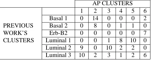
As in previous examples, a small plateau at six clusters is visible in Fig. 8. The distribution of patients in six clusters from AP compared with the one from the Sotiriou’s groups is reported in Table 8.

AP CLUSTERS

PREVIOUS WORK’S CLUSTERS

1 2 3 4 5 6

Basal 1 0 14 0 0 0 2

Basal 2 0 8 0 1 1 0

Erb-B2 0 0 0 0 0 7

Luminal 1 0 0 1 8 10 0

Luminal 2 9 0 10 2 2 0

Luminal 3 10 2 3 1 2 6

Table 8. The distribution of subjects between new and old classification (Sotiriou et al. data)

by samples in Clusters 4 and 5, luminal 2 in Cluster 3 and luminal 3 was mainly associated to Cluster 1 but presents several cases in other clusters as well.

4

Discussion

Cluster analysis is a powerful technique to explore com-plex diseases and improve prognosis. The recent literature on omic data is rich of new methods of cluster analysis able to deal with huge datasets. Moreover techniques of visual-izations are usually adopted to suggest the number of clus-ters [6].

At the same time many papers warn against the possible misuse of clustering techniques [10].

One of the main problems is the subjectivity of the analy-sis and the ability of clustering algorithms to create clusters even in absence of real structure.

The choice of the number of clusters is one of the main problems to be faced when applying this kind of analysis. The possibility to use algorithms that incorporate a criterion for the choice of the optimal partition is one of the achieve-ment of the recent developachieve-ments in this research field. The Affinity Propagation algorithm is characterized by a simple software implementation and it has the ability to suggest the cluster number. In addition, this algorithm has the advan-tage of taking into account real data points as exemplars; in this way, also categorical data may be analysed using, as similarity, a different distance from the Euclidean one. By looking for a set of exemplars, and not for a set of cen-troids, the search space is restricted, improving the compu-tational efficiency of the Affinity Propagation. In this work it was demonstrated how the algorithm is in agreement with the solutions obtained with much more effort with tradi-tional algorithms and indexes for the cluster number choice. Moreover the range of the suggested solutions gives insights in the hierarchical structure of the data highlighting differ-ent level of information for the treatmdiffer-ent of cancer patidiffer-ents well in accordance with previous knowledge. In particu-lar the solution with two clusters for Ferrara breast cancer

data, evidenced in Fig. 1, reflects the well known separation between tumors ER positive and negatives. This is a very important distinction and, in fact, in a number of paper of the pre-genomic era the number of clusters considered was in fact two [20, 18]. The solution with four clusters is in agreement with the solution selected in the previous work and the four clusters obtained are similar to that created by the PAM algorithm. The solution with five clusters sug-gests a possible more complex pattern to be explored. The clustering obtained by AP on the melanoma data is able to reproduce the interesting findings of Bittner and colleagues having the advantage of avoiding any arbitrary choice due to the visual inspection of the dendrogram. Over Perou et al. the AP could almost reproduce previous classifica-tion: the basal-like tumours were captures by Cluster 1, and the normal-like ones were assigned to Cluster 2; Clusters 3 and 4 represent the luminal-epithelial tumours, while the Erb-B2 group was not identified by AP in a single cluster. The solution with two clusters for van’t Veer et al. data reflects with a few number of exceptions, the separation be-tween ER+ and ER- groups evidenced in the original work. Applying AP over the dataset of Sotiriou and colleagues, four groups were evident and it was also possible to charac-terised them on the basis of gene expression of the tumour markers. AP Clusters 1 and 3 were associated with high val-ues of luminal cytokeratins and overexpression of ER, while Cluster 2 presents an overexpression of the basal CKs and low levels of ER. For Cluster 4 was not possible to obtain a distinctive characterisation, as it presented similar features to the overall population.

In conclusion, it is worth noting that, for the last three datasets analysed, a common solution in 6 clusters emerged by the AP algorithm, while one in 4 groups was not evident in van’t Veer et al. work.

As a future work, the characterisation of the AP groups on the basis of gene expressions will be carried out and compare with the one obtained in the original papers.

Acknowledgments

This study, was in part, funded by the BIOPTRAIN FP6 Marie-Curie EST Fellowship (FP6-007597).

References

[1] F. Ambrogi, E. Biganzoli, P. Querzoli, S. Ferretti, P. Borac-chi, S. Alberti, E. Marubini, and I. Nenci. Molecular sub-typing of breast cancer from traditional tumor marker pro-files using parallel clustering methods. Clinical Cancer

Re-search, 12(3):781–790, 2006.

[3] M. Bittner, P. Meltzer, Y. Chen, Y. Jiang, E. Seftor, M. Hen-drix, M. Radmacher, R. Simon, Z. Yakhini, A. Ben-Dor, N. Sampas, E. Dougherty, E. Wang, F. Marincola, C. Gooden, J. Lueders, A. Glatfelter, P. Pollock, J. Carpten, E. Gillanders, D. Leja, K. Dietrich, C. Beaudry, M. Berens, D. Alberts, V. Sondak, N. Hayward, and J. Trent. Molecu-lar classification of cutaneous malignant melanoma by gene expression profiling. Nature, 406:536–540, 2000.

[4] R. Calinski and J. Harabasz. A dendrite method for cluster analysis. Communs statist, 3:1–27, 1974.

[5] D. Dueck, B. Frey, N. Jojic, V. Jojic, G. Giaever, A. Emili, G. Musso, and R. Hegele. Constructing Treatment Portfolios

Using Affinity Propagation, volume 4955 of Lecture Notes in Computer Science, pages 360–371. Springer Berlin /

Hei-delberg, 2008.

[6] M. Eisen, P. Spellman, P. Brown, and D. Botstein. Clus-ter analysis and display of genome-wide expression patClus-terns.

Proc Natl Acad Sci U S A, 95:14863–8, 1998.

[7] B. Frey and D. Dueck. Mixture Modeling

by Affinity Propagation. Freely available at

http://books.nips.cc/papers/files/nips18/NIPS2005 0799.pdf. [8] B. Frey and D. Dueck. Clustering by passing messages

be-tween data points. Science, 315(5814):972–6, 2007. [9] G. Getz, E. Levine, and D. E. Coupled two-way clustering

analysis of gene microarray data. Proc Natl Acad Sci U S A, 97(22):12079–84, 2000.

[10] D. Goldstein, G. Debashis, and E. Conlon. Statistical issues in the clustering of gene expression data. Statistica Sinica, 12:219–240, 2002.

[11] M. Greenacre. Theory and Applications of Correspondence

Analysis. Academic Press, 1994.

[12] J. Hartigan. Clustering Algorithms. Wiley series in prob-ability and mathematical statistics. Applied Probprob-ability and Statistics. New York: Wiley, 1975.

[13] L. Kaufman and P. Rousseeuw. Finding Groups in Data:

an Introduction to Cluster Analysis. Wiley series in

prob-ability and mathematical statistics. Applied Probprob-ability and Statistics. New York: Wiley, 1990.

[14] W. Krzanowski and Y. Lai. A criterion for determining the number of clusters in a data set. Biometrics, 44:23–34, 1985. [15] N. Lama, F. Ambrogi, L. Antolini, P. Boracchi, and E. Bi-ganzoli. Some issues and perspective in microarray data analysis in breast cancer: the need for an integrated research. In Proceedings of the 1st European Workshop on the

Assess-ment of Diagnostic Performance, 2004.

[16] L. Lebart, A. Morineau, and M. Piron. Statistique

Ex-ploratoire Multidimensionnelle. Dunod, Paris, 1995.

[17] M. Leone, Sumedha, and M. Weigt. Clustering by

soft-constraint affinity propagation: Applications to gene-expression data. Bioinformatics, 23:2708–2615, 2007. [18] S. Mnard, P. Casalini, G. Tomasic, S. Pilotti, N. Cascinelli,

R. Bufalino, F. Perrone, C. Longhi, F. Rilke, and M.

Col-naghi. Pathobiologic identification of two distinct breast

carcinoma subsets with diverging clinical behaviors. Breast

Cancer Res Treat, 55(2):169–77, 1999.

[19] C. Perou, T. Sorlie, M. Eisen, M. Van De Rijn, S. Jef-frey, C. Rees, J. Pollack, D. Ross, H. Johnsen, L. Akslen,

O. Fluge, A. Pergamenschikov, C. Williams, S. Zhu, P. Lon-ning, A. Borresen-Dale, P. Brown, and D. Botstein. Molecu-lar portraits of human breast tumours. Nature, 406:747–752, 2000.

[20] P. Querzoli, S. Ferretti, G. Albonico, E. Magri, D. Scapoli, M. Indelli, and I. Nenci. Application of quantitative analy-sis to biologic profile evaluation in breast cancer. Cancer, 76(12):2510–7, 1995.

[21] R. Simon, E. Korn, L. McShane, M. Radmacher, G. Wright, and Y. Zhao. Design and Analysis of DNA Microarray

In-vestigations. Springer, 2004.

[22] C. Sotiriou, S.-Y. Neo, L. McShane, E. Korn, P. Long, A. Jazaeri, P. Martiat, S. Fox, A. Harris, and E. Liu. Breast cancer classification and prognosis based on gene expres-sion profiles from a population-based study. Proc Natl Acad

Sci USA, 100:10393–10398, 2003.

[23] R. Tibshirani, G. Walther, and T. Hastie. Estimating the number of clusters in a data set via the gap statistic. J.R.

Statist. Soc., B,63:411–423, 2001.

[24] O. Troyanskaya, M. Cantor, G. Sherlock, P. Brown, T. Hastie, R. Tibshirani, D. Botstein, and R. Altman. Miss-ing value estimation methods for DNA microarrays.

Bioin-formatics, 17(6):520525, 2001.

[25] L. van’t Veer, H. Dai, M. van de Vijver, Y. He, A. Hart, M. Mao, H. Peterse, K. van der Kooy, M. Marton, A. Wit-teveen, G. Schreiber, R. Kerkhoven, C. Roberts, P. Linsley, R. Bernards, and S. Friend. Gene expression profiling pre-dicts clinical outcome of breast cancer. Nature, 415:530– 536, 2002.

[26] W. Venables and B. Ripley. Modern Applied Statistics with