Evolutionary Local Search for Solving the
Office Space Allocation Problem
¨
Ozg¨ur ¨
Ulker
Automated Scheduling, Optimisation and Planning (ASAP) Research Group
School of Computer Science University of Nottingham Nottingham, NG8 1BB, UK Email: [email protected]
Dario Landa-Silva
Automated Scheduling, Optimisation and Planning (ASAP) Research Group
School of Computer Science University of Nottingham Nottingham, NG8 1BB, UK Email: [email protected]
Abstract—Office Space Allocation (OSA) is the task of correctly allocating the spatial resources of an institution to a set of entities by minimising the wastage of space and the violation of additional constraints. In this paper, an evolutionary local search algorithm is presented to tackle this problem. The evolutionary components of the algorithm include standard crossover and mutation operators and a relatively small population of indi-viduals. The offspring produced by the evolutionary operators are subjected to a short but intense local search process. A very fast cost calculation method tailored for searching a large section of the search space is implemented. Extensive experimentation is carried out related to several parameters of the algorithm: the mutation rate, the population size, the length of the local search procedure after each mutation, hence the balance between the evolutionary and the local search stages, and the level of greediness of the local search process. The final results on 72 different data instances show that this hybrid evolutionary algorithm is very competitive with an integer programming model.
I. INTRODUCTION
Office Space Allocation (OSA) is the task of distributing the space (rooms, floors, halls) used in an organisation to a set of entities (people, machines) based upon a set of constraints and objectives. While the main target in a typical OSA problem is to reduce the misuse of space, additional constraints that involve the relationships between several entities and rooms can arise in different problem variants. Several attributes of the problem can be traced back to thebin packing[1],multiple knapsack [2], andgeneralised assignment [3] problems.
Now in this paper, an evolutionary local search algorithm (ELS) is described for tackling the OSA problem. This al-gorithm combines evolutionary mechanisms of crossover and mutation (to move around the search space) with a fast and extensive local search procedure (to quickly search through a specific segment of the search space). The proposed method is competitive with a mathematical programming approach [4] developed previously for tackling this combinatorial optimisa-tion problem.
The initial attempts at tackling the office space allocation problem were several goal and linear programming approaches by Ritzman et al. [5], Benjamin et al. [6], and Giannikos et al. [7]. A systematic analysis of the problem was done by
Burke and Varley [8] in a questionnaire about the manual space allocation process in 38 UK universities. This questionnaire depicted some of the most commonly encountered constraints and objectives that are also investigated here.
Burke et al. [9] applied various hill climbing and simulated annealing [10] methods to solve the optimisation (creating a complete allocation from scratch) andreorganisationproblems by using allocation, reallocation and swap moves. In the follow up works, [11] and [12], the authors combined their local search methods within a population based framework. A mutation operator was also implemented for the disruption of the current solution. The authors concluded that the population based algorithm did not offer any benefits over the variant tailored for creating a single higher quality solution. Burke et al. [13] further reported the application of multi-objective optimisation by using two different objectives (the total space misuse in an allocation and the weighted sum of the soft constraints violated). It is reported that these two objectives were conflicting in nature.
Landa-Silva and Burke [14] developed an asynchronous cooperative local search method in which several local search threads in a population cooperated with each other to improve the solution. In the information sharing strategy, promising segments of the solution were shared between different threads and the diversification strategy applied a mutation operator over the bad regions of the solution. The authors implemented hill climbing, simulated annealing, and a hybrid metaheuristic within a population based framework.
minimisation of the misallocation of the rooms.
Ulker and Landa-Silva [17] developed a 0-1 integer pro-gramming [18] model based upon the office space alloca-tion problem variant described in [19]. The first model was implemented using CPLEX [20] as an integer programming solver. This model yielded the best obtained results for the larger dataset instances that were used in [19] and [14]. The model was later improved in [4] with a different not sharing
constraint formulation and the addition of three different constraint types that were not present in previous works. The model was reimplemented using Gurobi [21] and improved results over [17] were observed. Additionally, a random data instance generator was presented. Two new datasets were created by starting with an initial set of entities, rooms and constraints and modifying them via four different parameters which adjusted the difficulty of the instance.
This paper is organised as follows: Section II explains the problem definition of the OSA variant in this paper. Section III is devoted to the details of the ELS algorithm. Section IV presents extensive experimentation on two different datasets. Finally, Section V presents final remarks about the current algorithm and provides further research directions.
II. PROBLEM DEFINITION
A typical OSA problem contains three important sets: The
E set contains information related to the entities (the space required for the entity, the organisational group it belongs to, constraints associated with it, etc). The R set contains the attributes of each room (the capacity of the room, the floor it is in, the neighbourhood relationships with other rooms, the capacity constraints associated with it, the space that is currently being used, etc). Finally the Cset represents all the constraints (hard and soft) associated to entities and the rooms. There are two main goals in the variant of the office space allocation problem [19] considered in this paper: the minimisation of the space misuse and the minimisation of the soft constraint violations. The space misuse is the summation of the under and over utilisation of the rooms beyond their capacity. Since it is not desirable for the rooms to be overused beyond their capacity, the overuse of a room is penalised twice as much as under-utilisation of a room. In certain cases, it is not even possible to overuse a room at all. On the other hand, it is not desirable for a large number of rooms being under-utilised. In such allocations, it might be preferable to remove these severely under-utilised rooms from the problem, and redo the allocation task with the remaining rooms.
There are additional constraints that can happen frequently in many organisations. Nine types of such constraints are considered in this paper. These constraints can be eitherhard
(must be satisfied all the time) or soft (desirable but not necessary). These constraints are defined in Table I.
The difference between the adjacency and nearby con-straints is that the adjacency constraint is related to rooms that are really close to each other, whereas thenearbyrelation deals with rooms that in a larger neighbourhood (like a floor or a specific large section of a building).
TABLE I
DESCRIPTION OF THE CONSTRAINTS
Type Description Weight
allocation eshould be in roomr 20 non-allocation eshould not be in roomr 10 same room e1ande2should be in same room 10
not same room e1 ande2should not be in same room 10
not sharing eshould not share its room with others 50 adjacency e1 ande2should be in adjacent rooms 10
nearby e1ande2 should be in nearby rooms 10
away from e1 ande2should be away from each other 10
capacity rshould not be overused 10
In this work, the objective function that has to be minimised is taken as in [19]: the weighted sum of the space misuse and the soft constraint violations. The space misuse penaltympin a given solution is:
mp=
|R|
X
i=1
max((cap(ri)−usg(ri),2×(usg(ri)−cap(ri)))
(1) wherecap(ri)andusg(ri)stand for the capacity and the used space of roomri respectively.
The soft constraint violation penaltycpis the weighted sum of the individual soft constraint violations which is
cp=
|C|
X
i=1
w(ci)×v(ci) (2)
wherev(ci) = 1if the constraint is violated andv(ci) = 0if the constraint is satisfied. The total penaltytpthen becomes
tp=α×mp+β×cp (3)
whereαandβ are selected as 1.0 for this work.
III. THEALGORITHM
In this work, an evolutionary local search algorithm, also referred as a memetic algorithm, was developed. A memetic algorithm [22] is traditionally the hybridization of a genetic algorithm [23] with local search mechanisms. The goal of the evolutionary components of the algorithm is typically jumping to a different region of the search space. The local search is then applied to quickly explore this specific region of the search space.
A. Evolutionary Components
Input: input file with entities, rooms, and constraints.
Output: solution (an entity-room mapping)
Randomly Select Two Individuals for Crossover Apply Crossover to produce two offspring Apply Random Mutation on the two offspring Apply Allocation Mutation on the two offspring Apply Local Search on the two offspring
[image:3.612.316.543.72.367.2]Replace the parents with the best solution encountered so far in ELS.
Fig. 1. Evolutionary Local Search Algorithm
crossover as well as problem specific crossovers (based upon the preservation of the allocations within the rooms and the floors), we did not observe any tangible benefits of using these, that is why this paper restricts itself to the traditional one point crossover. After the crossover, two types of mutation operations are applied to the produced offspring. The first one is the traditional random mutation operator in which a randomly selected location is changed (which effectively sends the entity from one room to another). The mutation rate m (which is the percentage of the entities that are randomly subjected to mutation) is an important parameter of the algorithm. The second mutation operator is based upon the allocation constraint. The operator selects a randomly high number of violated allocation constraints and forces them to be satisfied by setting the corresponding location in the individual accordingly. After the two mutation operators, the offspring is improved using the local search procedure. Finally, the best obtained solution encountered during the search replaces the parent.
B. Local Search
Our main design goal with the local search operator is to apply a short but aggressive search to cover the single-move neighborhood of a candidate solution as quickly as possible. We implemented a local search method based upon searching a large portion of the single-move (one entity to another room) neighbourhood of the current solution as fast as possible.
For an efficient implementation of this greedy local search, fast cost calculations that involve the space misuse and the nine different types of constraint violations are required. We used a
∆matrix of size|E||R|where each location(e, r)corresponds to a move of sending the entity efrom its current location to another room r and holds the cost change of making such a move. There are two steps to maintain the∆matrix: delta and update stages.
C. Delta Stage
This stage is the initial calculation of the ∆matrix given a current solution. This stage incrementally calculates the whole single-move neighbourhood of a candidate solution. It is a costly operation and must be used once after a large change is made on the candidate solution. In our algorithm, this is the first step in the local search phase after the crossover and the mutation operators are applied to the individual.
Input: input solution
Output: output solution
Initial calculation of thedeltamatrix (Delta Stage)
for= 1→hiterationsdo
SelectE0 =|E|/dentities randomly from the entity set Find minimum(e, r2)in∀e∈E0 ∀r∈R (e, r)
Make move(e, r1, r2)
Update the locations in∆affected by the move(e, r1, r2)
end for
Fig. 2. Local Search Stage
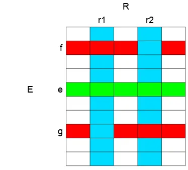
R
r1 r2
f
E e
g
Fig. 3. Locations affected by the move(e, r1, r2). Theerow, andr1and
r2columns are always affected in each iteration. The update onfandgrows
depends upon the constraint and the allocations inr1andr2
D. Update Stage
After a single move (e, r1, r2) has been applied to the
solution (entityeis moved from roomr1tor2), certain regions
of the ∆ matrix have to be updated. The algorithm goes through all constraints associated to the entity e, and rooms
r1 andr2 and only updates the locations that are affected by
this single move(e, r1, r2). The affected locations (illustrated
in Figure 3) are as follows:
When an entity eis moved from room r1 to r2, we must
check whether there should be a change of space misuse when moving the rest of the entities to these two rooms,r1 andr2.
This corresponds to the locations ∀e0 ∈ (E−e)(e0, r1) and
(e0, r2)in ∆ matrix. Since the space usage in r1 is going to
be reduced and the space usage inr2is going to be increased,
the algorithm checks the difference of the space misuse of sending the entities ∀e0 ∈ (E−e) to r1 and r2 before and
after the move is made and updates the corresponding location accordingly. Additionally, the locations ∀r ∈ (R−r2) f ∈
Er1(f, r)and∀r
0 ∈(R−r
1)g∈Er2(g, r
0)also need to be
updated. This corresponds to sending an entity that is already present in eitherr1 orr2 to all the other rooms and updating
the space misuse accordingly.
[image:3.612.330.517.199.368.2]in space misuse calculations described above. The algorithm checks whether affected rooms have space overuse before and after the move, whether moving the other entities to roomsr1
orr2prevents or causes an overuse before and after the move,
and updates the corresponding locations accordingly.
For the not sharing constraint (that an entity should not share a room with others), the locations ∀e0∈(E−e)(e0, r1)
and (e0, r2) need to be updated because of the number of
entities in rooms r1 and r2 are changed. Sending any other
entity to r1 or r2 might change the not sharing penalty if
the roomsr1andr2contain entities that should not share the
rooms with others. Additionally, the locations ∀r∈(R−r2)
f ∈ Er1(f, r) and∀r
0 ∈ (R−r
1) g ∈ Er2(g, r
0) might or
might not require an update operation.
If the entity e has any of same room, not same room,
adjacency, nearby, and away from constraints with another entity f, then the locations ∀r ∈ R (f, r) need updating. These locations correspond to the moves that send the entity
f to other rooms. If the constraint is satisfied before the move and not satisfied later or in the opposite case (that the constraint is not satisfied before the move and now it is satisfied), depending upon the constraint, the respective constraint penalty should be either subtracted or added to
∀r∈R (f, r).
During our experiments, it was observed that roughly three to five percent of the∆ matrix needs to be updated whenever a move is made. This percentage is expected to go down if the number of rooms is increased. As a result, the update stage will result in very high speedups for algorithms that search a large portion of the search space at each iteration (such as tabu search or steepest descent). However, it is not desirable to use the update stage in algorithms that operate on the acceptance or rejection of random moves (such as Simulated Annealing).
E. Partial Local Search
During the local search stage, the ∆ matrix is calculated first. At each one of the h iterations, a random subset E0 of
entities of size |E|/d is selected, and the minimum location
(e, r) is searched in that subsection of the ∆ matrix. The d
paramater adjusts the greediness of this search: when d = 1, the whole neighbourhood is checked. However, in practice poor results were observed with such a greedy search, that is why additional experiments with different values of d were performed.
F. Tabu Search
As an alternative to the local search, we also implemented a tabu search [24] procedure. Tabu search algorithm utilises a data structure called atabu list to prevent certain moves from being carried out to prevent the search getting stuck in local optima. In our implementation, whenever an entityeis moved from roomr1 tor2, the moves that send the entity back to r1
are considered tabuand hence forbidden until the end of that specific local search stage. However if a tabu move produces the best obtained solution encountered during the entire search, the move is made (aspiration criteria).
TABLE II
ATTRIBUTES OF THE INSTANCES INSVE150ANDPNE150DATASETS
Attribute Value
Number of entities: 150 Entity size: 5.5 - 30.5 Number of Groups: 10
Number of Floors: 3 Number of Rooms: 92 Number of Hard Constraints: 67
Number of Soft Constraints: 185 - 214
IV. EXPERIMENTS
The algorithm was implemented using the Microsoft Visual Studio 2010 C++ compiler. All experiments were carried out on a Windows PC with Intel Core 2 Duo E8400 (3 Ghz) processor.
In our experiments, we used the SVe150 and PNe150
datasets from [4]. These datasets contain 150 entities and 92 rooms and were incrementally generated from initial sets of entity, rooms, and constraints using four different parameters. The S (slack space) and V (soft constraint violation) rates adjust the amount of space misuse and soft constraint violation penalties in an instance respectively and higher values of S
and V amount to higher space misuse and soft constraint violation penalties. The P (positive slack) and N (negative slack) rates adjust the amount of space underuse and space overuse penalties respectively. Higher values of P and N
amount to higher space underuse and overuse penalties. The
SVe150 dataset contains 36 instances in which the S and V
rates change between 0.00 and 1.00 with 0.20 increments. The
PNe150dataset contains another 36 instances where theP and
N rates change between 0.00 and 0.25 with 0.05 increments. The attributes of theSV e150andP N e150instances are given in Table II.
In order to determine the best parameter values form (ran-dom mutation rate),h (the number of local search iterations after each mutation), d (divisor value which adjusts the size of the neighbourhood explored by the local search in each iteration) andps(population size), we performed initial experi-ments on 6 instances chosen fromSVe150andPNe150. These instances are S0.00V0.00, S0.40V0.80, S0.80V0.40, P0.00N0.00,
P0.10N0.20 and P0.20N0.10. In these experiments, each
in-stance was given 20 runs of 90 seconds each for a total execution time of 30 minutes. Our base parameter values were
m= 0.03,h= 100,d= 3 andps= 20 unless one of them was changed in its respective test.
Four different mutation rates (m = 0.00, m = 0.01,
m= 0.03,m= 0.05) and four different values for number of iterations after each mutation (h = 50, h = 100 h = 250,
h = 500) were tested. Since a large mutation rate might cause a large disruption on the solution, there might be a need for a larger number of iterations afterwards to obtain better results. The results are given in Table III and V for
TABLE III
THE IMPACT OF DIFFERENT M(MUTATION RATE)ON INSTANCES S0.00V0.00,S0.40V0.80ANDS0.80V0.40
instance m µ σ min max
S0.00V0.00
0.00 677.35 200.09 241.50 1107.50 0.01 64.35 19.42 38.50 111.00 0.03 51.85 20.91 24.00 92.00 0.05 52.33 18.84 22.50 84.50
S0.40V0.80
0.00 755.83 188.12 412.20 1158.10 0.01 239.47 20.13 211.50 278.30 0.03 230.49 14.90 205.50 253.20 0.05 243.77 22.11 208.90 286.30
S0.80V0.40
0.00 841.56 209.57 505.50 1242.10 0.01 199.24 16.64 171.30 249.00 0.03 198.99 17.38 171.60 239.60 0.05 204.43 15.51 186.40 243.90
TABLE IV
THE IMPACT OF DIFFERENT M(MUTATION RATE)ON INSTANCES P0.00N0.00,P0.10N0.20ANDP0.20N0.10
instance m µ σ min max
P0.00N0.00
0.00 760.75 229.60 297.50 1046.50 0.01 111.25 19.22 82.00 146.50 0.03 116.88 23.52 78.00 161.50 0.05 110.93 17.74 79.00 141.50
P0.10N0.20
0.00 787.31 154.35 574.30 1059.60 0.01 228.22 12.25 209.30 256.50 0.03 226.18 16.94 196.10 261.70 0.05 231.74 16.07 207.00 275.20
P0.20N0.10
0.00 688.20 215.08 353.70 1032.90 0.01 173.17 19.82 143.80 207.50 0.03 167.27 17.14 145.30 205.70 0.05 178.24 17.43 144.50 215.70
the number of local search iterations respectively. Columns
µ, σ, min and max represent the average best objective value, the standard deviation on the best objective value, the minimum and maximum objective value obtained after 20 runs respectively.
It was observed that the mutation was essential to the success of the algorithm; without random mutation (the case
m= 0.00), the algorithm quickly got stuck in a local optimum and produced uncompetitive results. We observed that the algorithm worked best when the mutation rate was around (m= 0.01−0.03), althoughm= 0.05still yielded acceptable results. It was observed that the local search iterations should be kept quite low (usually h = 50, h = 100) for the best results to be obtained. Increasing h beyond 500 affected the performance of the algorithm adversely, therefore, using a long extensive local search after each crossover and mutation operator is not recommended. Another benefit of using a lower
[image:5.612.331.543.86.265.2]h is that it reduced the effect of using different mutation rates between m = 0.01 and m = 0.05, therefore, setting the mutation rate precisely becomes less important.
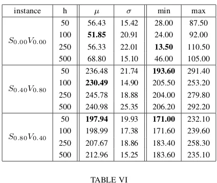
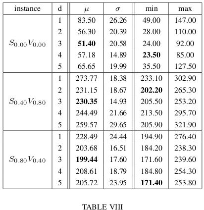
Table VII and Table VIII depict the effect of using different
TABLE V
THE IMPACT OF DIFFERENT H(LOCAL SEARCH ITERATIONS)ON INSTANCESS0.00V0.00,S0.40V0.80ANDS0.80V0.40
instance h µ σ min max
S0.00V0.00
50 56.43 15.42 28.00 87.50 100 51.85 20.91 24.00 92.00 250 56.33 22.01 13.50 110.50 500 68.80 15.10 46.00 105.00
S0.40V0.80
50 236.48 21.74 193.60 291.40 100 230.49 14.90 205.50 253.20 250 245.78 18.88 204.00 279.80 500 240.98 25.35 206.20 292.20
S0.80V0.40
50 197.94 19.93 171.00 232.10 100 198.99 17.38 171.60 239.60 250 207.67 18.86 183.40 258.30 500 212.96 15.25 183.60 235.10
TABLE VI
THE IMPACT OF DIFFERENT H(LOCAL SEARCH ITERATIONS)ON INSTANCESP0.00N0.00,P0.10N0.20ANDP0.20N0.10
instance h µ σ min max
P0.00N0.00
50 117.78 18.23 92.50 168.50 100 116.88 23.52 78.00 161.50 250 127.98 23.61 87.50 175.00 500 126.43 18.42 97.50 166.50
P0.10N0.20
50 225.84 12.42 207.20 246.70 100 226.18 16.94 196.10 261.70 250 240.57 24.55 216.40 298.70 500 245.79 23.06 204.00 278.10
P0.20N0.10
50 174.15 17.96 133.50 208.50 100 167.27 17.14 145.30 205.70 250 171.14 15.78 146.50 207.00 500 176.58 17.13 145.50 201.10
d(divisor) values on theSV andP N instances. Five different values were tested:d= 1(%100),d= 2(%50),d= 3(%33),
TABLE VII
THE IMPACT OF DIFFERENT D(DIVISOR)VALUES ON INSTANCES S0.00V0.00,S0.40V0.80ANDS0.80V0.40
instance d µ σ min max
S0.00V0.00
1 83.50 26.26 49.00 147.00 2 56.30 20.39 28.00 110.00 3 51.40 20.58 24.00 92.00 4 57.18 14.89 23.50 85.00 5 65.65 19.99 35.50 127.50
S0.40V0.80
1 273.77 18.38 233.10 302.90 2 231.15 18.67 202.20 265.30 3 230.35 14.93 205.50 253.20 4 244.49 21.66 213.50 295.70 5 259.57 29.65 205.90 321.90
S0.80V0.40
1 228.49 24.44 194.90 276.40 2 203.68 16.51 184.20 238.30 3 199.44 17.60 171.60 239.60 4 208.61 18.79 184.80 254.30 5 205.72 23.95 171.40 253.80
TABLE VIII
THE IMPACT OF DIFFERENT D(DIVISOR)VALUES ON INSTANCES P0.00N0.00,P0.10N0.20ANDP0.20N0.10
instance d µ σ min max
P0.00N0.00
1 134.93 14.00 108.00 159.00 2 118.03 13.06 91.00 138.50 3 117.45 23.10 78.00 161.50 4 132.10 20.96 98.00 173.50 5 120.33 19.34 82.00 146.50
P0.10N0.20
1 256.54 16.68 217.20 288.50 2 229.00 19.64 201.80 275.80 3 225.96 17.05 196.10 261.70 4 236.48 16.07 206.90 266.00 5 246.22 21.03 200.30 291.80
P0.20N0.10
1 215.03 23.89 172.00 255.60 2 178.51 26.73 144.40 228.80 3 167.12 16.80 145.30 202.70 4 174.12 16.64 149.90 212.90 5 169.94 20.07 140.60 212.30
rooms) is increased because the time required for searching the ∆ matrix is inversely proportional to d while the time required for the update stage is just directly proportional to the number of constraints (and hence mostly constant).
Our final parameter tests were performed on the ps, the number of individuals in a population. The population sizes were chosen as ps = 5, ps = 10, ps = 20, ps = 50 and
ps = 100. The results for SV and PN instances are given in Table IX and Table X respectively. It was observed that for the average best objective function value µ, there wasn’t any statistically significant difference between any of the ps
values. However, forps= 20individuals, it was observed that the chance of finding a best minimum value after 20 runs was slightly higher. The main benefit of using a population-based algorithm is to keep a number of different solutions so that
TABLE IX
THE IMPACT OF DIFFERENT PS(POPULATION SIZES)ON INSTANCES S0.00V0.00,S0.40V0.80ANDS0.80V0.40
instance ps µ σ min max
S0.00V0.00
5 52.63 16.11 33.00 98.00 10 58.30 16.68 31.00 82.50 20 51.40 20.58 24.00 92.00 50 63.28 24.99 28.50 109.50 100 49.80 20.34 16.50 99.50
S0.40V0.80
5 237.45 14.21 202.80 268.60 10 241.33 16.90 206.40 278.10 20 230.94 14.98 206.40 253.20 50 246.35 23.00 200.40 290.20 100 245.74 17.79 214.80 272.30
S0.80V0.40
5 203.72 16.59 182.70 239.10 10 201.01 13.82 177.90 226.90 20 199.34 17.49 171.60 239.60 50 208.02 17.95 173.80 247.00 100 204.41 16.69 185.70 239.30
TABLE X
THE IMPACT OF DIFFERENT PS(POPULATION SIZES)ON INSTANCES P0.00N0.00,P0.10N0.20ANDP0.20N0.10
instance ps µ σ min max
P0.00N0.00
5 117.23 13.52 97.50 146.50 10 119.40 13.85 95.00 146.00 20 116.88 23.52 78.00 161.50 50 118.43 25.58 79.00 173.00 100 116.10 15.39 87.50 140.50
P0.10N0.20
5 226.54 16.28 201.30 261.80 10 223.87 12.78 198.50 248.70 20 226.18 16.94 196.10 261.70 50 226.88 14.31 205.80 261.40 100 232.62 17.66 202.80 273.40
P0.20N0.10
5 167.77 16.53 140.20 195.30 10 162.21 12.14 139.50 190.60 20 167.27 17.14 145.30 205.70 50 167.85 12.94 141.90 189.90 100 165.65 16.57 144.00 207.40
the algorithm has a chance to backtrack from a local optimum to another section of the search space by means of crossover and mutation operators.
In Table XI, the comparison of using tabu search instead of local search within the evolutionary framework is presented. Columnsµ,σandmingive the average best objective value, the standard deviation on the best objective value and the minimum best objective value obtained after 20 runs of 90 seconds each. Replacing the local search with the tabu search offered no benefits for obtaining better average or minimum results. After using a small population, crossover and mutation operators and a divisor parameter to adjust the greediness of the search, adding a tabu list structure did not offer any additional benefit over the local search.
experimenta-TABLE XI
RESULTS ON SOME OF THESVANDPNINSTANCES USINGLOCAL AND TABUSEARCH WITHIN THEELS
Local Search Tabu Search
instance µ σ min µ σ min
S0.00V0.00 53.65 18.16 19.50 64.40 23.38 34.50
S0.40V0.80 233.62 23.27 190.70 248.48 14.99 209.00
S0.80V0.40 200.34 15.03 168.90 211.59 20.05 188.20
P0.00N0.00 108.65 19.55 74.00 123.03 17.21 90.00
P0.10N0.20 227.01 18.83 201.30 253.17 21.93 215.10
P0.20N0.10 165.25 14.78 140.50 190.22 14.97 165.80
tion on a subset ofSVe150andPNe150, additional experiments were carried out on the full set of instances. The following parameters were used: mutation rate m = 0.03, population size ps= 20, the number of local search iterationsh= 100
and the divisor value of the local search d= 3. Each instance was given 10 runs of 3 minutes each (for a total of 30 minutes execution time per instance). The results produced by the evolutionary local search algorithm were compared to the integer programming (IP) model proposed in [17] and [4]. The IP model had been given a single run of 30 minutes [4] using Gurobi’s deterministic IP solver [21]. In order to compare the new algorithm with the IP model, we took the minimum results obtained after ten runs. The Tables XII and XIII represent the results obtained. ColumnsS,V,P,N represent the four different parameters:slack space rate,soft constraint violation rate,positiveandnegative slack ratesrespectively. Columnsµ
andσrepresent the average and standard deviation of the total penalty obtained after 10 runs respectively. Columns mpand
cpgive the average misuse and soft constraint violation penalty after 10 runs respectively. Column min gives the minimum total penalty obtained after 10 runs and columnIPrepresents the best result obtained with the IP model [4].
For theSVe150dataset, out of the 36 instances, evolutionary local search algorithm produced better results for 21, and the IP formulation was more successful for the remaining 15 of them. It was observed that when the S and V were higher (when the expected space misuse and soft constraint violation penalty were higher in an instance), the ELS performed better than the IP formulation. However ELS struggled especially when the V value was low and it was beaten by the mathe-matical model in those cases. When V was low, the ELS had difficulty in reducing the space misuse penalty in an instance. However when the instance was expected to have higher space misuse and constraint violation penalties due to higherS and
V, the ELS performed better than IP.
There was a tie between the ELS and the IP with thePNe150
dataset. For 17 instances, ELS performed better, for the other 17 instance IP performed better and for the remaining two, there was a tie. Although there was not a clear pattern, it was observed that for lowP values (where the instance is expected to have small space underuse to compensate for the overuse), the IP performed better, however when P was increased, a more balanced outcome between the ELS and IP was observed.
TABLE XII
THE EXPERIMENTAL RESULTS ON THESVE150DATASET INSTANCES
s v µ σ mp cp min IP
0.00 0.00 49.30 15.11 39.30 10.00 31.50 0.00 0.00 0.20 90.80 27.30 52.80 38.00 61.50 32.00 0.00 0.40 102.40 17.43 56.40 46.00 89.50 57.00 0.00 0.60 118.40 12.31 50.40 68.00 99.00 95.50 0.00 0.80 169.85 18.04 65.85 104.00 138.50 171.00 0.00 1.00 192.25 18.89 65.25 127.00 165.00 193.00 0.20 0.00 64.04 14.29 55.04 9.00 38.90 28.10 0.20 0.20 105.24 22.72 62.24 43.00 77.90 52.90 0.20 0.40 133.23 22.45 75.23 58.00 115.40 86.60 0.20 0.60 139.92 14.46 69.92 70.00 117.10 122.80 0.20 0.80 182.19 17.11 85.19 97.00 157.90 212.70 0.20 1.00 213.71 28.83 90.71 123.00 181.60 210.30 0.40 0.00 125.27 16.59 95.27 30.00 108.40 82.80 0.40 0.20 157.45 25.90 101.45 56.00 118.80 116.30 0.40 0.40 173.27 18.85 110.27 63.00 144.60 155.10 0.40 0.60 197.05 18.05 123.05 74.00 163.90 188.80 0.40 0.80 218.23 17.24 117.23 101.00 185.60 208.70 0.40 1.00 246.95 19.30 126.95 120.00 219.70 271.50 0.60 0.00 137.63 11.85 115.63 22.00 116.60 109.70 0.60 0.20 170.23 10.72 122.23 48.00 154.70 129.70 0.60 0.40 198.65 10.45 134.65 64.00 189.00 168.20 0.60 0.60 209.00 14.25 136.00 73.00 189.20 205.20 0.60 0.80 254.23 12.97 143.23 111.00 233.60 289.10 0.60 1.00 280.13 17.34 153.13 127.00 261.90 278.70 0.80 0.00 151.31 13.52 120.31 31.00 131.40 124.70 0.80 0.20 170.63 14.38 124.63 46.00 152.90 160.30 0.80 0.40 188.42 13.09 127.42 61.00 165.00 173.60 0.80 0.60 202.94 18.59 132.94 70.00 175.90 195.90 0.80 0.80 255.37 23.72 141.37 114.00 229.20 267.80 0.80 1.00 284.52 12.18 159.52 125.00 259.20 276.10 1.00 0.00 186.75 15.25 160.75 26.00 167.70 169.10 1.00 0.20 226.99 17.17 172.99 54.00 201.00 194.20 1.00 0.40 243.02 12.53 176.02 67.00 225.30 221.40 1.00 0.60 260.61 18.44 174.61 86.00 238.30 243.40 1.00 0.80 298.76 11.16 195.76 103.00 284.90 340.40 1.00 1.00 309.96 19.46 187.96 122.00 280.80 345.30
V. CONCLUSION ANDFUTUREWORK
In this paper, we presented an evolutionary local search algorithm to solve the office space allocation problem. This algorithm was designed to be a fast method to find high-quality solutions for this difficult and highly constrained combinatorial optimisation problem. In our experiments, it was observed that the mutation rate m and the number of local search iterationshturned out to be the performance affecting factors of the algorithm. Low mutation rates and a small number of local search iterations greatly improve the performance of the algorithm. When we compare the current evolutionary local search algorithm to the mathematical programming model presented in [4], for more than half of the instances, better results were obtained for the same execution times.
muta-TABLE XIII
THE EXPERIMENTAL RESULTS ON THEPNE150DATASET INSTANCES
p n µ σ mp cp min IP
0.00 0.00 103.75 14.60 45.75 58.00 79.00 73.00 0.00 0.05 138.90 9.06 79.90 59.00 120.80 119.40 0.00 0.10 174.45 9.22 117.45 57.00 161.70 145.20 0.00 0.15 216.14 12.34 153.14 63.00 198.40 186.00 0.00 0.20 244.64 17.54 183.64 61.00 222.90 210.20 0.00 0.25 283.79 10.31 220.79 63.00 269.20 250.80 0.05 0.00 111.01 21.50 55.01 56.00 87.90 119.90 0.05 0.05 133.29 13.50 76.29 57.00 113.90 130.80 0.05 0.10 173.08 16.11 108.08 65.00 146.90 141.40 0.05 0.15 201.85 17.62 135.85 66.00 180.40 185.00 0.05 0.20 227.66 14.74 168.66 59.00 206.60 202.40 0.05 0.25 268.28 11.81 204.28 64.00 250.60 232.70 0.10 0.00 128.74 19.64 60.74 68.00 100.50 130.40 0.10 0.05 142.71 23.96 82.71 60.00 106.00 134.00 0.10 0.10 169.92 17.08 105.92 64.00 149.40 162.60 0.10 0.15 203.62 13.83 134.62 69.00 182.40 176.30 0.10 0.20 217.43 17.65 155.43 62.00 192.20 205.00 0.10 0.25 254.31 15.28 192.31 62.00 237.00 240.60 0.15 0.00 116.55 13.32 64.55 52.00 91.50 96.00 0.15 0.05 136.17 15.01 82.17 54.00 120.20 105.40 0.15 0.10 157.63 11.56 104.63 53.00 143.50 124.50 0.15 0.15 185.43 13.92 123.43 62.00 159.30 183.50 0.15 0.20 219.86 17.90 151.86 68.00 203.10 192.90 0.15 0.25 236.59 12.55 176.59 60.00 213.70 229.50 0.20 0.00 119.61 11.29 73.61 46.00 108.60 108.60 0.20 0.05 148.65 10.12 94.65 54.00 138.90 135.40 0.20 0.10 155.50 12.12 105.50 50.00 141.70 129.90 0.20 0.15 186.63 18.79 127.63 59.00 161.50 167.20 0.20 0.20 204.08 11.13 142.08 62.00 184.10 177.20 0.20 0.25 236.96 23.25 166.96 70.00 204.40 219.50 0.25 0.00 139.03 12.99 89.03 50.00 126.00 126.00 0.25 0.05 150.55 9.51 101.55 49.00 133.90 180.30 0.25 0.10 164.91 12.96 115.91 49.00 151.20 132.90 0.25 0.15 185.92 9.77 125.92 60.00 170.70 192.40 0.25 0.20 199.60 7.71 132.60 67.00 189.80 195.30 0.25 0.25 233.41 13.21 158.41 75.00 212.40 233.00
tion operator, we used a mutation operator based upon the
allocation constraint. Although additional mutation operators based upon the correction and disruption of other types of constraints (mainlysame room,adjacency,nearby, andaway from) were implemented, our limited experimentation with these procedures did not yield immediate benefits. However, revisiting these mutation operators is planned because of the high penalty values in some of these constraints.
The current variant of the algorithm is tailored for shorter runs, our limited experimentation on longer runs did not offer any drastic improvement on the solution quality. Instead, in order to prevent the algorithm from getting stuck in a local optima, backtracking to a previous population in the search or a complete restart of the algorithm is being considered rather than letting the algorithm running indefinitely to improve the
current best solution.
REFERENCES
[1] E. G. Coffman, M. R. Garey, and D. S. Johnson, “Approximation algorithms for bin packing: A survey,” pp. 46–93, 1997.
[2] S. Martello and P. Toth,Knapsack problems: algorithms and computer implementations. New York, USA: John Wiley & Sons, Inc., 1990. [3] D. G. Cattrysse and L. N. Van Wassenhove, “A survey of algorithms for
the generalized assignment problem,”European Journal of Operational Research, vol. 60, no. 3, pp. 260–272, 1992.
[4] ¨O. ¨Ulker and D. Landa-Silva, “Designing difficult office space allocation problem instances with mathematical programming,” inSEA - Sympo-sium of Experimental Algorithms, 2011, pp. 280–291.
[5] L. Ritzman, J. Bradford, and R. Jacobs, “A multiple objective approach to space planning for academic facilities,”Managament Science, vol. 25, no. 9, pp. 895–906, 1980.
[6] C. Benjamin, I. Ehie, and Y. Omurtag, “Planning facilities at the university of missouri-rolla.”Interfaces, vol. 22, no. 4, 1992. [7] J. Giannikos, E. El-Darzi, and P. Lees, “An integer goal programming
model to allocate offices to staff in an academic instituition.”Journal of the Operational Research Society, vol. 46, no. 6, pp. 713–720, 1995. [8] E. K. Burke and D. B. Varley, “Automating space allocation in higher
education,” inSEAL’98: Selected papers from the Second Asia-Pacific Conference on Simulated Evolution and Learning on Simulated Evolu-tion and Learning. London, UK: Springer-Verlag, 1999, pp. 66–73. [9] E. K. Burke, P. Cowling, J. D. Landa Silva, and B. McCollum, “Three
methods to automate the space allocation process in UK universities,” inThe practice and theory of automated timetabling III (PATAT 2004), LNCS, Vol. 2079. Springer, 2001, pp. 254–273.
[10] S. Kirkpatrick, C. D. Gelatt, and M. P. Vecchi, “Optimization by simulated annealing,”Science, vol. 220, pp. 671–680, 1983.
[11] E. K. Burke, P. Cowling, and J. D. Landa Silva, “Hybrid population-based metaheuristic approaches for the space allocation problem,” in
Proceedings of the 2001 Congress on Evolutionary Computation (CEC 2001), 2001, pp. 232–239.
[12] E. K. Burke, P. Cowling, J. D. Landa Silva, and S. Petrovic, “Combining hybrid metaheuristics and populations for the multiobjective optimisa-tion of space allocaoptimisa-tion problems,” inProceedings of the 2001 Genetic and Evolutionary Computation Conference (GECCO 2001), 2001, pp. 1252–1259.
[13] E. K. Burke, J. D. Landa Silva, and E. Soubeiga,Multi-objective hyper-heuristic Approaches for Apace Allocation and Timetabling. Springer, 2005, pp. 129–158.
[14] D. Landa-Silva and E. K. Burke, “Asynchronous cooperative local search for the office-space-allocation problem,”INFORMS J. on Computing, vol. 19, no. 4, pp. 575–587, 2007.
[15] R. Lopes and D. Girimonte, “The office-space-allocation problem in strongly hierarchized organizations,” in Evolutionary Computation in Combinatorial Optimization, ser. LNCS. Springer, 2010, vol. 6022, pp. 143–153.
[16] R. Pereira, K. Cummiskey, and R. Kincaid, “Office space allocation optimization,” in IEEE Systems and Information Engineering Design Symposium (SIEDS 2010), 2010, pp. 112–117.
[17] ¨O. ¨Ulker and D. Landa-Silva, “A 0/1 integer programming model for the office space allocation problem,”Electronic Notes in Discrete Mathematics, vol. 36, pp. 575–582, 2010.
[18] L. A. Wolsey,Integer programming, 1st ed. Wiley Interscience, 1998. [19] J. D. Landa-Silva, “Metaheuristics and multiobjective approaches for space allocation,” Ph.D. dissertation, School of Computer Science and Information Technology, University of Nottingham, 2003.
[20] IBM, “Ilog cplex optimizer,” 2010. [Online]. Available: http://www-01.ibm.com/software/integration/optimization/cplex/
[21] G. Optimisation, “Gurobi,” 2010. [Online]. Available: http://www.gurobi.com
[22] P. Moscato, “On evolution, search, optimization, genetic algorithms and martial arts - towards memetic algorithms,” 1989.
[23] D. E. Goldberg, Genetic Algorithms in Search, Optimization, and Machine Learning, 1st ed. Addison-Wesley, 1989.