Different Feature Selection of Soil Attributes Influenced Clustering Performance on Soil Datasets

(1)

ISSN Online: 2156-8367 ISSN Print: 2156-8359

DOI: 10.4236/ijg.2019.1010052 Oct. 21, 2019 919 International Journal of Geosciences

Different Feature Selection of Soil Attributes

Influenced Clustering Performance on Soil

Datasets

Jiaogen Zhou

1

, Yang Wang

1,2

1_{School of Urban and Environmental Science, Huaiyin Normal University, Huai’an, China} 2_{Information Engineering School, Nanchang University, Nanchang, China}

Abstract

Feature selection is very important to obtain meaningful and interpretive clustering results from a clustering analysis. In the application of soil data clustering, there is a lack of good understanding of the response of clustering performance to different features subsets. In the present paper, we analyzed the performance differences between k-means, fuzzy c-means, and spectral clustering algorithms in the conditions of different feature subsets of soil data sets. The experimental results demonstrated that the performances of spectral clustering algorithm were generally better than those of k-means and fuzzy

c-means with different features subsets. The feature subsets containing envi-ronmental attributes helped to improve clustering performances better than those having spatial attributes and produced more accurate and meaningful clustering results. Our results demonstrated that combination of spectral clus-tering algorithm with the feature subsets containing environmental attributes rather than spatial attributes may be a better choice in applications of soil da-ta clustering.

Keywords

Feature Selection, K-Means Clustering, Fuzzy C-Means Clustering, Spectral Clustering, Soil Attributes

1. Introduction

Clustering generally divides a dataset (in which each data object has certain attributes) into k sub-clusters such that similar objects are within the same sub-cluster and dissimilar objects are in different sub-clusters [1]. Clustering How to cite this paper: Zhou, J.G. and

Wang, Y. (2019) Different Feature Selec-tion of Soil Attributes Influenced Cluster-ing Performance on Soil Datasets. Interna-tional Journal of Geosciences, 10, 919-929. https://doi.org/10.4236/ijg.2019.1010052

Received: August 25, 2019 Accepted: October 18, 2019 Published: October 21, 2019

(2)

DOI: 10.4236/ijg.2019.1010052 920 International Journal of Geosciences analysis often uses an unsupervised technique to extract interesting and useful information from large datasets without prior knowledge. To obtain good clus-tering results, we normally require relevant features to be included in the train-ing data and an appropriate clustertrain-ing method.

In real conditions, the observation objects generally have multiple features collected in different ways. The selection of useful, relevant features and removal of redundant features are important preprocessing steps in clustering analysis. Generally, ideal features should be useful in distinguishing patterns belonging to different clusters, immune to noise, easy to extract and interpret, decrease the workload, and simplify the subsequent design process [2]. The selection of ap-propriate features ensures meaningful and interpretive results. Although a number of methods for selecting appropriate feature subsets have been developed and reviewed [3], there is still an absent understanding of the influence of different feature subsets on the clustering performance in the real applications of soil data clustering to our knowledge.

On the other hand, no single clustering method presents a panacea that can be applied in all clustering conditions. Thus, different clustering methods have been developed to solve specific clustering problems [1][4]. In the fields of agricul-ture and soil, clustering analysis has been applied to recognize soil patterns [5] [6][7], manage soil nutrients [8][9], design good soil sampling strategies [10] [11], and identify soil microbial communities [12][13] [14], etc. However, few studies have compared the performance differences of clustering methods on soil data.

Inspired by the above-mentioned, we choose three classical clustering algo-rithms of k-means, fuzzy c-means, and spectral clustering, which are widely used and representative of the current state-of-the-art. To our best knowledge, we first evaluate the influence of different feature sets on the performances of the three clustering methods on soil data. Our research will provide a good reference for selecting a good combination of clustering algorithm and feature subsets in applications of soil data clustering.

2. Materials and Methods

2.1. Clustering Methods

K-means clustering is a very simple and widely applied clustering method. Given the observation data set O=

{

x x1, 2,,xn

}

, where each observation is a d-dimensional vector, k-means clustering partitions the n observations into k (≤ n) sub-sets. To achieve the optimal clustering result, k-means clustering minimizes the within-cluster sum of squares (WCSS) [1][4]. The clustering process has two steps: 1) first, randomly selects k observations as their initial mean or centers of sub-clusters. Each remaining data object will be assigned to the nearest sub- cluster based on the distance to each of the cluster centers, and the centers of the sub-clusters is then recalculated; 2) repeat (1) until WCSS is minimized.

(3)

ob-DOI: 10.4236/ijg.2019.1010052 921 International Journal of Geosciences ject must be placed into a cluster, but this can be simplified by considering a fuzzy property between observations. To represent the fuzzy boundaries between observations, fuzzy c-means clustering allows each observation to belong to more than one sub-cluster, and then associates the sub-clusters with a set of member-ship levels. Fuzzy c-means clustering first assigns the membership levels between observations and sub-clusters, and then uses these to allocate observations to one or more clusters. Fuzzy c-means clustering minimizes the following objec-tive function of WCSS [15]:

(

)

2

1 1

WCSS arg min

n k

ij i j i j

u x C

= =

=

∑∑

− ₍₁₎

where uij is the degree of membership of xi in cluster Cj, and Ciis the center of the cluster. In fuzzy clustering, the WCSS in (1) is iteratively optimized, and the membership uij and cluster center Ci are updated according to:

2 1 1 1 m k i j ij

l i l

x c u x c − = −   = _ _ −  

∑

(2)

1 1

n n

j ij i ij

i i

c u x u

= =

=

∑

₍₃₎

Spectral clustering was developed to handle data with any shape and ensure convergence to the global optimum. This method constructs an affinity graph which is partitioned according to the corresponding Laplace eigen-spectrum [16]. First, a graph is formed based on the similarity between observations. Each graph node corresponds to one observation, nodes are connected with edges, and the edge weights denote the degree of similarity between observations [17] [18]. The graph is further characterized by the adjacency matrix W.

Let the diagonal matrix D=

∑

Wij where Wij is a diagonal element, and de-fine the Laplacian matrix L = D − W. The top-k eigenvalues and corresponding eigenvector of L are calculated, and these k eigenvectors are arranged to form an

n × k matrix, where each row can be taken as a k-dimensional vector. Finally, the

k-means algorithm is applied to this n × k matrix, and the output is the spectral clustering result.

2.2. Selection of Feature Subsets

(4)

DOI: 10.4236/ijg.2019.1010052 922 International Journal of Geosciences feature subsets is both interesting and of practical importance when analyzing soil data.

We set six possible subsets of soil features: 1) spatial attributes (SA); 2) envi-ronmental variables (EV); 3) spatial attributes and envienvi-ronmental variables (SA + EV); 4) spatial attributes and soil condition variables (SA + SCV); 5) environmen-tal and soil condition variables (EV + SCV); and 6) the whole set of attributes (WA).

The environmental variables influencing the soil conditions of interest are the features contained in EV, SA + EV, EV + SCV, and WA. Note that not all envi-ronmental variables affect a certain soil condition. Hence, redundant environ-mental variables that are not related to the soil conditions of interest should be removed.

2.3. Data Acquisition and Preprocessing

Two real soil datasets both contain 520 soil samples collected in Pangtang Town, Taoyuan County, Hunan Province. These are used to verify the effect of different feature sets on clustering performance. Each soil sample in the two datasets con-tains five attribute fields: spatial position (x, y coordinates), terrain factors (ele-vation, slope), and a soil condition (SOC or soil pH). Before applying the clus-tering models, the values of all soil attributes were normalized according to:

( )

min

max min

j j

i i

j

i _j _j

i i

A A

NA

A A

− =

− (4)

where j i

A , min

( )

j i

A , and max

( )

j i

A denote the value of soil attribute j for soil sample i, the minimum value of soil attribute j, and the maximum value of soil attribute j, respectively.

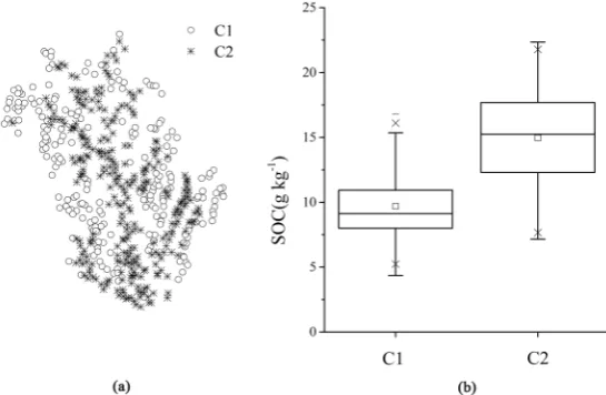
[image:4.595.211.535.534.692.2]

The spatial distribution of the soil samples and environmental variables (ele-vation and slope) are shown in Figure 1. In the soil datasets, SOC is highly cor-related with elevation and slope [20], but this is not the case for pH. Moreover, there is a significant difference between the SOC values in the top (elevation >

(5)

DOI: 10.4236/ijg.2019.1010052 923 International Journal of Geosciences 95 m) and bottom (elevation < 95 m) regions. Therefore, the dataset including SOC field can simply be divided into two sub-clusters according to the elevation threshold of 95 m. The spatial distribution of sub-clusters C1 and C2is shown in Figure 2(a). The box-plot clearly indicates a significant difference of SOC con-tents between C1 and C2 (Figure 2(b)).

2.4. Validation

The k-means clustering, fuzzy c-means clustering and spectral clustering algo-rithms were applied to the experimental datasets. Good clustering results should exhibit a significant difference between the soil conditions of interest in different sub-clusters. In this study, we use two indicators to evaluate the clustering per-formance: the clustering dissimilarity index (DI), and the root mean square of clustering dissimilarity index (RSDI).

(

2 1

)

k

i j

DI C C

k k ≠

= −

∗ −

∑

(5)

(

1 1

)

i

(

)

2

k

i j x C

RSDI C C

n k ≠ ∈

= −

∗ −

∑ ∑

(6)

where ˆ i

C and Cˆ_j are the average values of a certain soil condition in sub-clus-

ters Ci and Cj, respectively, k is the total number of clusters, C xi

( )

is the soil condition value of sample x in sub-cluster Ci, and n is the total number of soil samples.

[image:5.595.236.509.503.681.2]

DI and RSDI can reflect the difference of a certain soil condition between the various sub-clusters. The bigger these two index values are, the greater the dif-ferences of the soil condition between the sub-clusters. This indicates a better clustering result. For example, DI and RSDI were maximized when the dataset was partitioned into two sub-clusters by selecting an elevation threshold of 95 m in the case of the dataset of SOC (Figure 3).

(6)

DOI: 10.4236/ijg.2019.1010052 924 International Journal of Geosciences

Figure 3. Change in clustering dissimilarity index (DI and RSDI) with selected elevation values for grouping the soil dataset of SOC.

2.5. Programming Implementation

The k-means, fuzzy c-means, and spectral clustering algorithms were implemented in Matlab2010 on a Windows Xp operating system. The digital maps of soil sam-ples and topography factors were produced using ArcGis9.0.

3. Results and Discussion

3.1. Clustering Performance under Different Soil Feature Subsets

We tested the influence of different soil feature sets (SA, EV, SA + SCV, SA + EV, EV + SCV, and WA) on the clustering performance of the three clustering algorithms. For each soil feature set, the three clustering algorithms were ex-ecuted so as to form sub-clusters with respect to SOC. The spatial distribution of the soil samples in the resulting clusters clearly reflects the response of the clus-tering performance to the selection of different soil features.

Compared with the control (Figure 2(a)), the distributions of the clustered samples given by the three algorithms under the six feature subsets have signifi-cant differences. Under EV (Figure 4(d), Figure 4(j) and Figure 4(p)), EV + SCV (Figure 4(e), Figure 4(k) and Figure 4(q)) and WA (Figure 4(f), Figure 4(l) and Figure 4(r)), the clustered samples produced by all three clustering methods generally match the control. Under the SA + EV treatment, spectral clustering produces the clustering result that best matches the control (Figure 4(o)), followed by fuzzy c-means (Figure 4(i)), with k-means the worst perfor-mer (Figure 4(c)). Compared with the results for the above-mentioned feature subsets, SA and SA + SCV both resulted in worse clustering. Under SA and SA + SCV, all three clustering methods generated two sub-clusters that were scattered to the north or south and significantly deviated from the control.

(7)

[image:7.595.212.537.75.329.2]

Figure 4. Distribution of clusters generated by k-means (top), fuzzy c-means (middle), and spectral clustering (bottom) under six different feature subsets on the SOC dataset (from left to right: SA, SA + SCV, SA + EV, EV, EV + SCV, and WA). SA: spatial attributes; SA + SCV: spatial attributes and soil condition variables; SA + EV: spatial attributes and environmental variables; EV: environmental variables; EV + SCV: envi-ronmental and soil condition variables; and WA: the whole set of attributes.

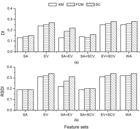
[image:7.595.232.514.421.681.2]

(8)

DOI: 10.4236/ijg.2019.1010052 926 International Journal of Geosciences demonstrates that EV, EV + SCV, and WA produced a better clustering than SA + EV, with SA and SA + SCV producing the worst results. Additionally, the clustering performance of each clustering method can differ under the same feature set. Overall, spectral clustering generated relatively higher values of DI

and RSDI than k-means and fuzzy c-means for EV, EV + SCV, SA + EV, and

WA, but not for SA and SA + SCV. This indicates that spectral clustering is more robust to changes in the feature sets than k-means and fuzzy c-means.

3.2. Influence of Correlation between Environmental Variables

and Soil Conditions on Clustering Performance

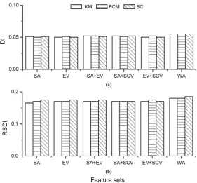
We also tested whether the pH values in each sub-cluster were significantly dif-ferent. DI and RSDI were again used to evaluate the deviation in pH values be-tween the two sub-clusters under different soil feature subsets. Generally speak-ing, the values of DI or RSDI are very similar for all six soil feature sets (Figure 6). Additionally, the clustering performance of the three clustering methods did not vary for the same feature set. This demonstrates that the resulted sub-clusters have no significant differences in pH under the six soil feature subsets considered here.

[image:8.595.233.515.418.679.2]

Regarding the topographical factors(elevation and slope) correlating well with SOC but not with pH, whether the feature subsets containing environmental factors help to improve clustering performance or not depends on the correla-tion of environmental attributes with one or more soil condicorrela-tions. In other words,

(9)

DOI: 10.4236/ijg.2019.1010052 927 International Journal of Geosciences feature subsets containing environmental variables help to improve clustering performance only if there is a significant relation between environmental va-riables and the soil conditions of interest. This assertion is supported by the fact that DI and RSDI (based on pH) exhibited no significant difference under six feature sub sets, whereas these indexes varied considerably with respect to SOC. Additionally, in the case of SOC, the bad clustering results under SA, SA + SCV, and SA + EV further suggest that spatial attributes make bad contributions in clustering models.

In many practical applications, environmental data collected by remote sens-ing techniques is rich and easily accessible, while relatively small amounts of soil condition data can be obtained at larger cost in terms of human resources and time. Thus, using environmental attributes that correlate well with soil con-ditions, rather than spatial attributes, will enable better recognition of soil pat-terns and allow information on soil conditions to be applied in the analysis of soil data.

4. Conclusion

The present study examined the effect of different soil feature subsets on the clus-tering performance. It was found that the feature subsets containing environ-mental variables generally helped to improve clustering performances of k-means, fuzzy c-means, and spectral clustering methods better than those having spatial attributes. Additionally, spectral clustering was clearly more robust to changes of feature sunsets than k-means and fuzzy c-means clustering methods in our study case. Thus, the combination of spectral clustering method with the feature sub-sets containing environmental variables can produce useful soil patterns when applied to soil survey data, especially those with an irregular shape. In future, diverse soil datasets will be used to further validate our results at a bigger spatial scale.

Acknowledgements

This study was jointly supported by National Natural Science Foundation of Chi-na (41877009, 41201299).

Conflicts of Interest

The authors declare no conflicts of interest regarding the publication of this pa-per.

References

[1] Jain, A.K., Murty, M.N. and Flynn, P.J. (1999) Data Clustering: A Reviewing. ACM Computing Surveys, 31, 264-323.https://doi.org/10.1145/331499.331504

[2] Blum, A.L. and Langley, P. (1997) Selection of Relevant Features and Examples in Machine Learning. Artificial Intelligence, 97, 245-271.

(10)

[3] Guyon, I. and Elisseeff, A. (2003) An Introduction to Variable and Feature Selec-tion. Journal of Machine Learning Research, 3, 1157-1182.

https://doi.org/10.1162/153244303322753616

[4] Xu, R. and Donald, W. (2005) Survey of Clustering Algorithm. IEEE Transactions on Natural Networks, 16, 645-678.https://doi.org/10.1109/TNN.2005.845141

[5] Young, F.J. and Hammer, R.D. (2000) Defining Geographic Soil Bodies by Land-scape Position, Soil Taxonomy and Cluster Analysis. Soil Science Society of Ameri-ca Journal, 64, 948-998.https://doi.org/10.2136/sssaj2000.643989x

[6] Araujo, S.R., Wetterlind, J., Dematte, J.A.M. and Stenberg, B. (2014) Improving the Prediction Performance of a Large Tropical vis-NIR Spectroscopic Soil Library from Brazil by Clustering into Smaller Subsets or Use of Data Mining Calibration Tech-niques. European Journal of Soil Science, 65, 718-729.

https://doi.org/10.1111/ejss.12165

[7] Triantafilis, J., Gibbs, I. and Earl, N. (2013) Digital Soil Pattern Recognition in the Lower Namoi Valley Using Numerical Clustering of Gamma-Ray Spectrometry Data.

Geoderma, 192, 407-421.https://doi.org/10.1016/j.geoderma.2012.08.021

[8] Davatgar, N., Neishabouri, M.R. and Sepashhah, A.R. (2012) Delineation of Site Specific Nutrient Management Zones for a Paddy Cultivated Area Based on Soil Fertility Using Fuzzy Clustering. Geoderma, 173-174, 111-118.

https://doi.org/10.1016/j.geoderma.2011.12.005

[9] Tripathi, R., Nayak, A.K., Shahid, M., Lai, B., Gautam, P., Raja, R., Mohanty, S., Kumar, A., Panda, B.B. and Sahoo, P.N. (2015) Delineation of Soil Management Zones for a Rice Cultivated Area in Eastern India Using Fuzzy Clustering. Catena, 133, 128-136.https://doi.org/10.1016/j.catena.2015.05.009

[10] Odeh, I.O.A., McBratney, A.B. and Chittleborough, D.J. (1990) Design of Optimal Sample Spacing for Mapping Soil Using Fuzzy-k-Means and Regionalized Variable Theory. Geoderma, 47, 93-122.https://doi.org/10.1016/0016-7061(90)90049-F

[11] Lin, Q.H., Li, H., Luo, W., Lin, Z.M. and Li, B.G. (2013) Optimal Soil Sampling De-sign for Rubber Tree Management Based on Fuzzy Clustering. Forest Ecology and Management, 308, 214-222.https://doi.org/10.1016/j.foreco.2013.07.028

[12] Goberma, M., Navarro-Cano, Banuet, A.V., Garcia, C. and Verdu, M. (2014) Abiot-ic Stress Tolerance and Competition-Related Traits Underlie PhylogenetAbiot-ic Cluster-ing in Soil Bacterial Communities. Ecology Letters, 17, 1191-1201.

https://doi.org/10.1111/ele.12341

[13] Deangelis, K.M. and Firestone, M.K. (2012) Phylogenetic Clustering of Soil Micro-bial Communities by 16S rRNA But Not 16S rRNA Genes. Applied and Environ-mental Microbiology, 78, 2456-2461.https://doi.org/10.1128/AEM.07547-11

[14] Powers, Z.C., Owen, J.G., Reddy, B.V., Ternei, M.A. and Brady, S.F. (2014) Chemi-cal-Biogeographic Survey of Secondary Metabolism in Soil. PNAS, 111, 3757-3762.

https://doi.org/10.1073/pnas.1318021111

[15] Wu, K.L. and Yang, M.S. (2002) Alternative c-Means Clustering Algorithms. Pat-tern Recognition, 35, 2267-2278.https://doi.org/10.1016/S0031-3203(01)00197-2

[16] Luxburg, U.V. (2007) A Tutorial on Spectral Clustering. Statistics and Computing, 17, 395-416.https://doi.org/10.1007/s11222-007-9033-z

[17] Li, J.Y., Zhou, J.G., Huang, W.J., Zhang, J.Z. and Yang, X.D. (2010) Grouping Ob-jects in Multi-Band Images Using an Improved Eigenvector-Based Algorithm. Ma-thematical and Computer Modeling, 51, 1332-1338.

(11)

[18] Shi, J. and Malik, J. (2000) Normalized Cuts and Image Segmentation. IEEE Trans-actions on Pattern Analysis and Machine Intelligence, 22, 888-905.

https://doi.org/10.1109/34.868688

[19] Zhu, A.X. (2000) Mapping Soil Landscape as Spatial Continua: The Neural Network Approach. Water Resources Research, 36, 663-677.

https://doi.org/10.1029/1999WR900315

[20] Liu, S.L., Li, Y., Wu, J.S., Huang, D.Y., Su, Y.R. and Wei, W.X. (2010) Spatial Varia-bility of Soil Microbial Biomass Carbon, Nitrogen and Phosphorus in a Hilly Red Soil Landscape in Subtropical China. Soil Science and Plant Nutrition, 56, 693-704.