arXiv:gr-qc/0101107 27 Jan 2001
INTEGRABILITY FOR RELATIVISTIC SPIN NETWORKS
JOHN C. BAEZ AND JOHN W. BARRETT
Abstract. The evaluation of relativistic spin networks plays a fundamental role in the Barrett-Crane state sum model of Lorentz-ian quantum gravity in 4 dimensions. A relativistic spin network is a graph labelled by unitary irreducible representations of the Lorentz group appearing in the direct integral decomposition of the space ofL2 functions on three-dimensional hyperbolic space.
To ‘evaluate’ such a spin network we must do an integral; if this integral converges we say the spin network is ‘integrable’. Here we show that a large class of relativistic spin networks are integrable, including any whose underlying graph is the 4-simplex (the com-plete graph on 5 vertices). This proves a conjecture of Barrett and Crane, whose validity is required for the convergence of their state sum model.
1. Introduction
In formulating a state sum model for 4-dimensional Lorentzian quan-tum gravity, Barrett and Crane [11] used the notion of a ‘relativistic spin network’, which is simply a graph with edges labelled by non-negative real numbers. These numbers parametrize a certain class of irreducible unitary representations of the Lorentz group. The model involves a triangulation of spacetime, and for each 4-simplex one must calculate an amplitude associated to a relativistic spin network whose underlying graph is the complete graph on 5 vertices:
• •HHH
HHHHHH •vvvv
vvvv v •) )) )) ) )) ) • H H H H H H H H H H H H H H v v v v v v v v v v v v v v )) )) ) )) )) )) )) )
converges whenever the underlying graph of the spin network lies in a certain large class. This class of graphs includes the tetrahedron and all graphs obtained from it by repeatedly adding an extra vertex connected by at least 3 edges to the existing graph. Thus in particular this class includes the complete graph on 5 vertices.
The results of the paper are formulated in Section 2 and proved in Section 3. These sections are developed in a self-contained manner, so that the reader interested in the mathematical details can simply start there.
The remainder of the introduction contains some background ma-terial placing the results in their mathematical and physical contexts. The mathematical part of the introduction explains how the integrals we consider arise from the representation theory of the Lorentz group. The physics part of the introduction sketches how this representation theory has been used in constructing models of fundamental physics. 1.1. Mathematical context. Calculations in the representation the-ory of compact Lie groups are conveniently expressed in terms of dia-grams. Let a, b, ...,n and p, q ,... , z be representations of the group and A: a⊗b⊗. . .⊗n → p⊗. . .⊗z an intertwining operator (a lin-ear map which commutes with the action of the group). This can be represented by a diagram:
A
n . . .
. . .
z q
b a
p
Usually we fix some particular operators and represent them by dia-grams like this; these operators are called the elementary operators, or sometimes vertices, corresponding to the fact that the graph in the diagram has just one vertex.
These processes allow us to build various operators from the elemen-tary ones, with the description in terms of elemenelemen-tary operators being captured by a diagram: a graph with vertices labelled by elementary operators and a certain number of free ends on the bottom and top, corresponding to ‘inputs’ and ‘outputs’:
A
b p a
c B
q
r
The power of this method comes from the fact that relations between these intertwining operators correspond, in many cases, to deforma-tions of the diagram which can be interpreted as moving the vertices and edges in either two- or three-dimensional space (isotopies). This theory was developed to its fullest extent in the generalisation from compact Lie groups to a certain class of Hopf algebras, particularly the quantum groups. Since a diagram with no free ends corresponds to an intertwining operator from the trivial representation to itself, i.e. essentially just a complex number, such Hopf algebras yield invariants of knots and graphs embedded in three-dimensional space.
However in this paper we are concerned with a generalisation in a different direction, namely from compact to non-compact Lie groups, and study a particular class of unitary representations of the Lorentz group, SO0(3,1). The subscript here indicates the connected
compo-nent of SO(3,1) that contains the identity. This is the group covered by SL(2,C).
the ordinary trace of the identity operator is infinite. However we will show that there is another perfectly good notion of trace provided that the diagram is sufficiently connected.
The representations of the Lorentz group considered here are as fol-lows. There is one for each real number p ≥ 0. The Hilbert space of this representation (also denoted p) is the space of solutions to the equation∇2f =−(p2+ 1)f on three-dimensional hyperbolic space, H,
which have square-integrable boundary data on the sphere at infinity [11]. This Hilbert space is characterised by a reproducing kernel on H,
Kp(x, y), which is a smooth, bounded, symmetric integral kernel that solves the equation ∇2K =−(p2+ 1)K in both xand y. The formula
for K is given in Section 2. The Lorentz group acts by translations on this Hilbert space, and the resulting representation is unitary and irreducible.
The elementary operatorA: p1⊗ · · · ⊗pm →q1⊗ · · · ⊗qn is defined
by
f1⊗ · · · ⊗fm 7→
1 2π2
Z
H
Kq1(y1, z)· · ·Kqn(yn, z)f1(z)· · ·fm(z) dz
(1)
The result of applying the operator A is a function of the variables
y1, . . . , yn in H. However it is not clear that this function lies in the
Hilbert space q1 ⊗ · · · ⊗qn. For now, we simply consider the formal
expressions that are obtained by composing these operators. We post-pone the question about whether these converge to the consideration of closed diagrams (those with no free ends).
The operator A can be thought of as an integral operator, albeit with a distributional integral kernel,
A(x1, . . . , xm;y1, . . . , yn) =
(2)
1 2π2
Z
H
Kq1(y1, z)· · ·Kqn(yn, z)δ(z, x1)· · ·δ(z, xm) dz
with δ(x, y) the delta function for integration on H. With this nota-tion, the composition of operators consists of multiplying their kernels and integrating the common variables over H. The trace is naturally expressed using the integral kernels in the same way. For example, the trace of A over the first variable is
Z
H
A(z, x2, . . . , xm;z, y2, . . . , yn) dz.
trace both involve joining a free end at the bottom of the diagram to a free end on the top, the calculation always gives a factor of
Z
H
Kp(y1, x)δ(x, y2) dx=Kp(y1, y2)
for each internal edge, with variables y1, y2 corresponding to its two
vertices.
The operator for a diagram with just two free ends
y
y p
1
0 q
can be described as follows. Associate a variable yi ∈ H to each ver-tex in the diagram. Let E be the set of all edges in the interior of the diagram (i.e., not meeting the boundary box). The corresponding operator is
f 7→Z Y
i
dyi
2π2
Y
E K
!
Kq(y1, x)f(y0).
In the main body of the paper we consider closed diagrams, those with no free ends on the boundary rectangle. The naive idea for as-sociating a number, or evaluation, to this graph would be to take the trace of the previous graph. But this trace is always infinite. However, by Schur’s lemma
y
y p
1
0 q
= Λ
q
p
In what follows, we show that a good definition for the evaluation of the closed diagram
p
.
is the above constant Λ; this constant is given by a multiple integral of products of K’s which converges in many cases. This definition is presented afresh in Section 2 with no reference to the representation theory sketched here. In that section, it is shown that this gives an invariant of the graph which does not depend on the way in which the diagram is drawn in the plane, nor on which edge is chosen to break it into a diagram with two free ends.
1.2. Physics applications. The study of spin networks was initiated by Penrose [21] in the early 1970’s, as part of an attempt to a find a description of the geometry of spacetime that takes quantum mechanics into account from the very start. These spin networks were simply graphs with edges labelled by irreducible representations of SU(2) (i.e. spinsj = 0,12,1,32, . . .) and vertices labelled by intertwining operators. Such spin networks are also implicit in Ponzano and Regge’s state sum model of 3-dimensional quantum gravity, published in 1968 [23]. However, this was only realized much later [19].
The real surge of work on spin networks came in the early 1990’s, when they were generalized to other groups and even quantum groups. At this point, people began to use them systematically to construct topological quantum field theories. For example, Reshetikhin and Tu-raev [26] used spin networks to give a purely combinatorial description of Chern-Simons theory and prove that it satisfies the Atiyah axioms for a 3-dimensional TQFT. Shortly thereafter, Turaev and Viro [30] used them to construct a q-deformed version of the Ponzano-Regge model and prove that it, too, is a TQFT. We now recognize this theory as a Euclidean signature version of 3d quantum gravity with nonzero cosmological constant. Later, Crane and Yetter [13] used spin network technology to construct a state sum model of a 4d TQFT. This appears to be a quantization of BF theory with cosmological constant term.
also far more problematic theory: 4-dimensional quantum gravity. The success of spin network methods in constructing TQFTs prompted var-ious attempts to apply spin networks to 4d quantum gravity. These attempts came from two main directions.
The first was work on ‘loop quantum gravity’, an approach to the canonical quantization of Einstein’s equations. Here Rovelli and Smolin [27] realized that SU(2) spin networks embedded in a 3-manifold rep-resenting space can serve as an explicit basis of kinematical states. Using this basis they showed how to construct operators corresponding to observables such as the areas of surfaces and volumes of regions [28]. This work was soon made rigorous by Ashtekar, Lewandowski, Baez and others, and spin networks quickly became a standard tool in this field [1, 2, 3, 4, 5].
The second direction was work on state sum models of 4d quantum gravity. Models of this sort were proposed by Barrett and Crane, first in the Euclidean [10] and then in the Lorentzian signature [11]. Their orig-inal models involve a triangulation of a fixed 4-manifold representing spacetime, but there is also great interest in more abstract ‘spin foam models’, where there is no underlying manifold [6, 7, 16, 22]. Again, these models come in both Euclidean and Lorentzian versions. The Lorentzian versions are more physically realistic, but they involve extra difficulties due to the noncompactness of the Lorentz group SO0(3,1),
the solution of which forms the main topic of this paper.
2. Evaluating relativistic spin networks
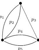
As discussed informally in the introduction, a relativistic spin net-work is a graph with an assignment of a real number p ≥ 0 to each edge. In what follows only relativistic spin networks whose underlying graph is connected are considered.
•
p2
p1 p
3
/ / / / / / / / // / / /
•
p4
p5
[image:7.595.274.341.581.665.2]•
The idea of an evaluation is a function that gives a number for each relativistic spin network. In [11] an integral was defined which deter-mines a number for the relativistic spin network, if it converges. The integral is based on the following kernel:
Kp(x, y) =Kp(r) = sinpr
psinhr
(3)
wherexandyare two points in three-dimensional hyperbolic space,H, and r is the distance between them. This formula defines the function
Kp(r) for p, r >0, but it extends uniquely to a continuous function of
p, r ≥0, withKp(0) = 1 and K0(r) =r/sinhr.
The integral is defined as follows. First, to each vertex v∈V of the graph we associate a variable xv ∈ H. Each edge e ∈E thus has two variables,xs(e)andxt(e), associated to its endpoints. Next, to each edge
e of the graph we associate a factor of Kp(xs(e), xt(e)), which depends
on the edge label p.
The idea is then to integrate the product of these factors QEK
over the variables in hyperbolic space. However, since this product is invariant under the action of SO0(3,1) as isometries of H, one of
the integrations is redundant, and would lead to an infinite value for the integral. Thus we arbitrarily choose one vertex, say w, and omit the integration over the variable associated to that vertex. Let V0 =
V − {w} be the remaining set of vertices, and n the total number of vertices.
The integral is then given as follows:
Iw(xw) = 1 (2π2)n−1
Z
Hn−1
Y
E
Kp(e)(xe(0), xe(1))
Y
v∈V0
dxv
(4)
The measure dx on hyperbolic space is the standard Riemannian vol-ume measure for the unit hyperboloid. In spherical coordinates where
r is the distance from a fixed origin
dx= sinh2rdrdΩ,
where dΩ is Lebesgue measure on the unit 2-sphere.
If the integral converges, it defines a function of the remaining vari-able, xw. However the Lorentz invariance gives Iw(xw) = Iw(L(xw)) for any L∈SO0(3,1), so the integral is actually a constant, say Iw.
The Lorentz invariance also implies that Iw is independent of the choice of the vertexw. This follows from the formula
Iw(xw) = Z
H
where the integrand is obtained by integrating over all but two vari-ables. This function is an invariant function on H×H, and therefore a function of the hyperbolic distance between its two arguments. Any such function is symmetric in its arguments. This establishes the equal-ityIw(xw) =Iv(xv).
Definition 1. The evaluation of a relativistic spin network is defined as the common value ofIw(xw)for any choice of vertex wandxw ∈H. Clearly this definition only works in the cases when the integral con-verges. We have not yet been precise about what this means. The best situation is when the integrand in the definition is integrable, i.e., when the Lebesgue integral of its absolute value exists. In this case we say that the relativistic spin network is integrable. The results in this paper refer to the integrable case. If the network is integrable for all values of the edge labelsp, then the graph will be called integrable, and the evaluation defines a function of these edge labels. Our first result is that this function is bounded:
Theorem 1. For an integrable graph, the relativistic spin network eval-uation is bounded by a constant that is independent of the edge labels.
A more general situation is where the integral defines a generalised function, or distribution, in the p variables. In this situation the rel-ativistic spin network may not be integrable for specific values of the edge labelsp. However, the integrand in the definition of the evaluation will become integrable after smoothing with suitable test functions in the p variables. We are not going to be precise about the details of the test functions, but will confine ourselves to noting some simple ex-amples where this phenomenon occurs. In this case, the graph will be called distributional. If the graph is not even distributional, it will be called divergent.
Some simple cases, calculated in [11], illustrate these definitions. A graph given by a single loop with one vertex on it:
•
p
has the evaluation
Kp(x, x) = 1.
A graph with two vertices on a loop:
•
a
b
has the evaluation 1
2π2
Z
H
Ka(x, y)Kb(y, x) dy= 2
πab
Z ∞ 0
sinarsinbrdr= δ(a−b)
a2 .
This is an example of a relativistic spin network that is not integrable for any values of a and b. However the result is well defined after smoothing in a and b, so the graph is distributional. In general this phenomenon occurs whenever the graph has a bivalent vertex.
In the simpler case of a closed network with two vertices joined with just one edge:
• p •
the evaluation is a divergent integral for all values of the label p. 1
2π2
Z
H
Kp(x, y) dy= 1 2π2p
Z ∞
0
sinhrsinprdr.
More generally, any graph with a univalent vertex is divergent. The theta graph with two vertices and three edges:
•
a
b c
•
is integrable and has the evaluation 1
2π2
Z
H
Ka(x, y)Kb(x, y)Kc(x, y) dy= 2
πabc
Z ∞ 0
sinarsinbrsincr
sinhr dr
= 1
4abc tanh( π
2(b+c−a)) + tanh(
π
2(c+a−b)) + tanh(π
2(a+b−c))−tanh(
π
2(a+b+c))
The graphs with two vertices and more than three connecting edges are also integrable and can be evaluated explicitly.
and call the complete graph on 5 vertices the ‘4-simplex’:
• •HHH
HHH HHH •vvvv
vvvv v •)) )) ) )) )) • H H H H H H H H H H H H H H v v v v v v v v v v v v v v )) ) )) )) )) )) )) )
Theorem 2. The tetrahedron is an integrable graph.
Theorem 3. A graph obtained from an integrable graph by connecting an extra vertex to the existing graph by at least three extra edges is integrable. A graph obtained from an integrable graph by adding extra edges is integrable. A graph constructed by joining two disjoint inte-grable graphs at a vertex is inteinte-grable.
Theorem 3 allows the construction of a large class of integrable graphs. Starting with a graph which is known to be integrable, such as the theta graph or the tetrahedron, then one can construct larger integrable graphs by successively carrying out the operations described in the theorem. In particular, the 4-simplex is integrable because it is obtained by adding a vertex connected by four edges to the tetrahe-dron.
3. Proof of the Main Results
In equation (4) we defined the evaluation of a relativistic spin net-work as a certain integral over n-tuples of points in hyperbolic space. To prove Theorems 2 and 3, we need to show this integral converges. Before starting the proofs, we give an informal outline of the procedure. Our procedure is to integrate over one point at a time, treating the remaining points as fixed. This is justified by the theorems of Fubini and Tonelli concerning the Lebesgue integral of a function of several variables [29].
For an example of this procedure, consider the integral Z
H
for fixedx1, . . . , xn∈H. To prove that this integral converges we need
a bound on the kernel K (proved below in Lemma 1): for any > 0, there exists a constantc (independent of p) such that
|Kp(r)| ≤ce−(1−)r.
Using this, it follows that the integral is bounded by
cn
Z
H
dx e−(1−)(r1+···+rn)
where ri = d(x, xi). Now suppose we can find a ‘barycentre’ for the points xi, that is, a pointb∈H such that
r:=d(x, b)≤ 1
n(r1+· · ·+rn)
for all x. Then if we work in spherical coordinates centered at b, we see that the integral is bounded by
4πcn
Z ∞ 0
e−(1−)nrsinh2rdr.
which converges for all n≥3 providing we pick 0 < <1/3.
This example illustrates the importance of adding 3 or more new edges for each new vertex in the graph. To prove our main results, we now prove the above bound on the kernel K, construct the required barycentres, and give an improved version of the above estimate. Fi-nally, we give a careful treatement of the tetrahedron graph.
We begin the formal proofs by boundingK. First note that|sinpr| ≤ pr so that for p > 0
|Kp(r)| = |sinpr|
psinhr ≤ r
sinhr.
(5)
This bound on Kp(r) also holds when r is zero, as long as we define
r/sinhr to equal 1 when r = 0. The right-hand side of the inequality is K0(r).
Proof of Theorem 1. By inequality 5, the evaluation of a relativistic spin network is bounded by the evaluation of the network with the edge labelp= 0 for each edge.
Now we give the detailed estimates needed for Theorems 2 and 3.
Lemma 1. For any >0, there exists a constant c such that |Kp(r)| ≤ce−(1−)r
Proof. Since the functionr/sinhris bounded and is asymptotic tore−r
as r→+∞, for any >0 there exists cwith
r
sinhr ≤ce
−(1−)r.
The second part follows because r/sinhr is bounded by 1.
Next we construct a barycentre for any finite collection of points in hyperbolic space, beginning with the case of two points.
Lemma 2. Supposep1, p2 ∈H and letpbe the midpoint of the geodesic
fromp1 to p2. For any point q∈H we have
d(p, q)≤ 1
2(d(p1, q) +d(p2, q)) Proof. Using notation as in this picture:
p 1 p
2 q
p r
1
r 2
r
we need to show r ≤ 1
2(r1 +r2). By the law of cosines for hyperbolic
trigonometry [24] we have
coshdcoshr = coshr1 + cosθsinhdsinhr,
coshdcoshr= coshr2 −cosθsinhdsinhr.
Adding these equations we obtain
coshdcoshr= cosh(r1−r2
2 ) cosh(
r1+r2
2 ). By the triangle inequality we have |r1−r2| ≤2d, so
coshr ≤cosh(r1+r2 2 ), from which the desired result follows.
A barycentre for 3 points can be constructed by an iterative process. Begin by constructing midpoints of the geodesics between the points
p1, p2 and p3 as in this picture:
p 1
2 p
p 1 p
p 3 p
2 3
Lemma 2 implies the inequality
d(p1, q) +d(p2, q) +d(p3, q)≥d(p01, q) +d(p02, q) +d(p03, q).
Iterating this process, we obtain a sequence of nested triangles in hy-perbolic space:
The vertices converge to a point p, the unique point contained in all the triangles. By repeated use of the above inequality
3d(p, q)≤d(p1, q) +d(p2, q) +d(p3, q),
so thatp is a barycentre.
The following constructions work for all n. First, consider the case where the points lie along a straight line, i.e. a geodesic γ ∈H. Then sinceγ is isometric to the real line with its usual metric, the arithmetric mean of the points is defined. The next lemma shows that this is a barycentre.
Lemma 3. Suppose γ ⊂H is a geodesic, andp1, p2, . . . , pn∈γ. Then
the arithmetic mean p of the points has the property that for any point
q∈H we have
d(p, q)≤ 1
Proof. This is proved by iteration. Suppose p1 and p2 are two points
in the set which are the farthest distance apart. Then using Lemma 2, we can replace both p1 and p2 by the barycentre of p1 and p2 without
increasing the quantity
d(p1, q) +d(p2, q) +· · ·+d(pn, q).
By iterating this process, all of the points in the set converge to the arithmetic mean p.
Now the main result on barycentres is proved.
Lemma 4. Suppose p1, p2, . . . , pn ∈ H. Then there exists a point p
such that for any point q∈H we have
d(p, q)≤ 1
n(d(p1, q) +d(p2, q) +· · ·+d(pn, q)).
Proof. This is proved by induction on n. The induction starts with
n = 2 by Lemma 2. Let b be a barycentre for the first n−1 points. Then by the induction hypothesis
(n−1)d(b, q) +d(pn, q)≤d(p1, q) +d(p2, q) +· · ·+d(pn, q).
Next we find a barycentre p for n −1 points at b and 1 point at pn. To do this, note that all these points lie on a geodesic, and so the barycentre is constructed by Lemma 3. We thus have
nd(p, q) ≤ (n−1)d(b, q) +d(pn, q)
≤ d(p1, q) +d(p2, q) +· · ·+d(pn, q).
Next we prove an improved version of the estimate given at the beginning of this section. Suppose x1, . . . , xn are fixed in H and rij =
d(xi, xj).
Lemma 5. If n ≥3, the integral
J = Z
H
dx|Kp1(x, x1)Kp2(x, x2)· · ·Kpn(x, xn)|
converges, and for any 0< <1/3 there exists a constant C > 0 such that for any choice of the points x1, . . . , xn,
J ≤C exp −n−2−n
n(n−1) X
i<j rij
Proof. Defineri =d(xi, x). Using Lemma 1 we obtain |Kp1(x, x1)· · ·Kpn(x, xn)| ≤c
ne−(1−)Pri.
If we work in spherical coordinates using the barycentre of the points
x1, x2, . . . , xn as our origin, this implies
J ≤4πcn
Z ∞ 0
e−(1−)
P
risinh2rdr.
We next break this integral over r into two parts, and estimate these separately using two bounds:
X
ri ≥nr
from Lemma 4, and
X
ri ≥nM
where
M = 1
nminx
X
ri.
We obtain
J ≤ 4πcn
Z M
0
e−n(1−)M sinh2rdr+ Z ∞
M
e−n(1−)rsinh2rdr
≤ 4πcn
Z M
0
e−n(1−)M+2rdr+
Z ∞
M
e−n(1−)r+2rdr
≤ Ce−(n−2−n)M
for some constant C > 0 depending only on and n. Finally, the triangle inequality implies
X
ri ≥ 1 n−1
X
i<j rij
for all choices of x1, x2, . . . , xn, so
M ≥ 1
n(n−1) X
i<j rij.
Adding an extra edge does not affect the integrability of a graph because |K|<1, by Lemma 1.
Finally, for two integrable graphs joined by identifying one vertex we have that the evaluation of the resulting graph is the product of the evaluations of the two pieces, and so in particular the graph is integrable. This follows from taking the vertex where the two pieces are joined as the vertex which is not integrated over in the definition of the evaluation.
By using Lemma 5 to evaluate a bound for the integral one vertex at a time, one can actually prove that the n-simplex is integrable for
n ≥5. However to do the important cases of the tetrahedron and the 4-simplex requires a more sensitive bound at the stage where there are 3 vertices.
Proof of Theorem 2. We need to show for any choice of numberspij ≥0 for 1 ≤i < j ≤4 and a point x1 ∈H, the integral
I = Z
H3
dx2dx3dx4 |Kp12(x1, x2)Kp13(x1, x3)Kp14(x1, x4) Kp23(x2, x3)Kp24(x2, x4)Kp34(x3, x4)|
converges.
First we integrate out x4 using Lemma 5, obtaining
I ≤C
Z
H2
dx2dx3 e− 1
6(1−3)(r12+r13+r23)|Kp
12(x1, x2)Kp13(x1, x3)Kp23(x2, x3)|
where rij =d(xi, xj).
Next integrate over another variable, say x3. With
L= Z
H
dx3 e− 1
6(1−3)(r13+r23)|Kp
13(x1, x3)Kp23(x2, x3)|
this gives
I ≤C
Z
H
dx2 L e− 1
6(1−3)r12|Kp
12(x1, x2)|.
(6)
By equation (5) we have
L ≤ Z
H
dx3
r13r23e− 1
6(1−3)(r13+r23)
sinhr13sinhr23
≤ Z
H
dx3
(r13+r23)2e− 1
6(1−3)(r13+r23)
sinhr13sinhr23
To get a good bound on the integral here, we resort to a coordinate system in which two of the coordinates are
k = 1
2(r13+r23), `= 1
2(r13−r23),
while the third is the angle φ betweenx3 and a given plane containing
the geodesic between x1 and x2. The ranges of these coordinates are
r/2≤k < ∞, −r/2≤` ≤r/2, 0≤φ <2π,
where we set r = r12. Coordinates of this sort can also be defined
in Euclidean space, where they are closely akin to prolate spheroidal coordinates [20], but here all the formulas are a bit different, since we are working in hyperbolic space. The main thing we need is a formula for the volume form in these coordinates,
dx3= 2
sinhr13 sinhr23
sinhr dkd`dφ
which is proved in the Appendix.
Using this formula we can do the integral (7) in the (k, `, φ) coordi-nate system, obtaining
L≤8 Z 2π
0
dφ
Z ∞
r/2
dk
Z r/2 −r/2
d` k
2e−1 3(1−3)k
sinhr
or doing the integral over φ and ` and then k,
L ≤ 16πr
sinhr
Z ∞
r/2
k2e−13(1−3)kdk
≤ (Ar
3 +B)e−16(1−3)r
sinhr
(8)
for some constants A and B independent of all the parameters in this problem.
We conclude the proof by using this bound onLto bound the integral
I. By (5) and (6) we have
I ≤ C
Z
H
dx2 L e− 1
6(1−3)r|Kp
12(x1, x2)|
≤ 4πC
Z ∞ 0
L re−16(1−3)rsinhrdr
and by (8) this gives
I ≤4πC
Z ∞ 0
r(Ar3+B)e−13(1−3)rdr.
4. Remarks and Conclusions
Theorem 3 gives a large class of integrable graphs, starting with the theta and tetrahedron graphs. However there are further examples of integrable graphs. For example, the graph in Figure 1 is also integrable, but cannot be constructed from any integrable graph by the methods of Theorem 3. Its integrability follows by applying Lemma 5 to one of the trivalent vertices.
It seems reasonable to conjecture that any 3-edge-connected graph is integrable. A 3-edge-connected graph is one that remains connected when any edge is removed or any pair of edges are removed.
It seems that the bound in Theorem 1 should be dramatically im-proved. Indeed, K satisfies the bound |K| <1/(psinhr) for r > 1/p, thus for largep one expects the evaluation to behave like 1/p for each edge variable. By inspection, this is the case for the theta-graph. We conjecture that a similar bound is true for all graphs not containing edge-loops (edges with both ends at the same vertex).
It would also be interesting to consider the obvious generalization of this theory to other dimensions. For applications to quantum gravity, one would want the (n+ 1)-simplex to be an integrable graph when labelled by any representations of SO0(n,1) appearing in the direct
integral decomposition of the space of L2 functions on n-dimensional
hyperbolic space.
5. Appendix: Spheroidal Coordinates in Hyperbolic Space
If we fix two pointsx1, x2 in three-dimensional hyperbolic space, and
pick a hyperbolic plane containing the geodesic between these points, we can define spheroidal coordinates on hyperbolic space as follows. Given any point x3 in hyperbolic space, its first two coordinates are
k = 1
2(r13+r23), `= 1
2(r13−r23),
where rij is the distance from xi to xj. The third coordinate is the angleφ betweenx3 and a given plane containing the geodesic between
x1 and x2. The ranges of these coordinates are
r/2≤k < ∞, −r/2≤` ≤r/2, 0≤φ <2π,
where we set r=r12.
In these coordinates, the volume form on hyperbolic space is given by
dx3 = 2
sinhr13 sinhr23
To prove this, it is easiest to consult the following picture and use the method of infinitesimals (or differential forms):
x 1
a 1 a
2
r 23 r
23
x 3 r
13
2 r
13
x
θ θ
d d
The area of the infinitesimal parallelogram formed as we vary r13 and
r23by amounts dr13and dr23is sinθ a1a2, whereθ is the angle between
the geodesics from x3 to x1 and x2. Evidently sinθ ai = dri3, so this
area is dr13dr23/sinθ = 2dkd`/sinθ. As we vary θ by an amount dθ,
this parallelogram sweeps out an infinitesimal paralleliped of volume dx3 = 2
sinhy
sinθ dkd`dφ,
where y is the distance from x3 to the geodesic between x1 and x2.
With the help of the following picture:
x 1
x 1
r 23
2 r
13
x θ
y
r
repeated use of the hyperbolic law of sines gives sinhy= sinhr13 sinhr23
sinhr sinθ
and thus
dx3 = 2
sinhr13 sinhr23
References
[1] A. Ashtekar and J. Lewandowski, Quantum theory of geometry I: area opera-tors,Class. Quantum Grav.14(1997), A55-A81.
[2] A. Ashtekar and J. Lewandowski, Quantum theory of geometry II: volume operators,Adv. Theor. Math. Phys.1(1998), 388-429.
[3] A. Ashtekar, A. Corichi and J. Zapata, Quantum theory of geometry III: non-commutativity of Riemannian structures, Class. Quantum Grav. 15 (1998), 2955-2972.
[4] J. C. Baez, Spin networks in gauge theory,Adv. Math.117(1996), 253–272. [5] J. C. Baez, Spin networks in nonperturbative quantum gravity, inThe
Inter-face of Knots and Physics, ed. L. Kauffman, American Mathematical Society, Providence, Rhode Island, 1996.
[6] J. C. Baez, Spin foam models,Class. Quantum Grav.15(1998), 1827–1858. [7] J. C. Baez, An introduction to spin foam models of quantum gravity and BF
theory, inGeometry and Quantum Physics, eds. Helmut Gausterer and Harald Grosse, Springer, Berlin, 2000.
[8] J. C. Baez and J. W. Barrett, The quantum tetrahedron in 3 and 4 dimensions, Adv. Theor. Math. Phys.4(1999), 815–850.
[9] J. W. Barrett, The classical evaluation of relativistic spin networks, Adv. Theor. Math. Phys.2(1998) 593–600.
[10] J. W. Barrett and L. Crane, Relativistic spin networks and quantum gravity, J. Math. Phys.39(1998) 3296–3302.
[11] J. W. Barrett and L. Crane, A Lorentzian signature model for quantum general relativity,Class. Quantum Grav.17(2000), 3101–3118.
[12] J. W. Barrett, R. M. Williams. The asymptotics of an amplitude for the 4-simplex,Adv. Theor. Math. Phys.3(1999), 209–214.
[13] L. Crane and D. Yetter, A categorical construction of 4d TQFTs, inQuantum Topology,eds. L. Kauffman and R. Baadhio, World Scientific, Singapore, 1993, pp. 120-130.
[14] L. Crane and D. Yetter, On the classical limit of the balanced state sum, preprint available as gr-qc/9712087.
[15] S. Davids, Semiclassical limits of extended Racah coefficients,J. Math. Phys.
41(2000), 924–943
[16] R. De Pietri, L. Freidel, K. Krasnov, C. Rovelli, Barrett-Crane model from a Boulatov-Ooguri field theory over a homogeneous space,Nucl. Phys. B574
(2000), 785–806.
[17] L. Freidel and K. Krasnov, Simple spin networks as Feynman graphs,J. Math. Phys.41(2000) 1681–1690.
[18] L. Freidel, K. Krasnov and R. Puzio, BF description of higher-dimensional gravity theories, preprint available as hep-th/9901069.
[19] B. Hasslacher and M. Perry, Spin networks are simplicial quantum gravity, Phys. Lett.B103(1981), 21-24.
[20] P. Moon and D. E. Spencer, Field Theory Handbook: Including Coordinate Systems, Differential Equations, and Their Solutions, Springer, Berlin, 1988. [21] R. Penrose, Angular momentum: an approach to combinatorial space-time, in
[22] A. Perez and C. Rovelli, Spin foam model for Lorentzian general relativity, preprint available as gr-qc/0009021.
[23] G. Ponzano and T. Regge, Semiclassical limit of Racah coefficients, in Spec-troscopic and Group Theoretical Methods in Physics, ed. F. Bloch, North-Holland, New York, 1968.
[24] J. G. Ratcliffe,Foundations of Hyperbolic Manifolds, Springer, Berlin, 1994. [25] M. Reisenberger, On relativistic spin network vertices, J. Math. Phys. 40
(1999), 2046–2054.
[26] N. Reshetikhin and V. Turaev, Invariants of 3-manifolds via link polynomials and quantum groups,Invent. Math.103(1991), 547–597.
[27] C. Rovelli and L. Smolin, Spin networks in quantum gravity,Phys. Rev.D52
(1995), 5743-5759.
[28] C. Rovelli and L. Smolin, Discreteness of area and volume in quantum gravity, Nucl. Phys.B442(1995), 593-622. Erratum,ibid.B456(1995), 753.
[29] H. L. Royden,Real Analysis, Macmillan, New York, 1988.
[30] V. Turaev and O. Viro, State sum invariants of 3-manifolds and quantum 6j
symbols,Topology31(1992), 865–902.
[31] D. Yetter, Generalized Barrett-Crane vertices and invariants of embedded graphs,J. Knot Theory Ramifications8(1999), 815–829.
Department of Mathematics, University of California, Riverside CA 92507, USA