Large eddy simulation of a three dimensional hypersonic shock wave turbulent boundary layer interaction of a single fin

Large-Eddy Simulation of a Three-Dimensional Hypersonic

Shock Wave/Turbulent Boundary Layer Interaction of a

Single-Fin

Jian Fang1 and Lipeng Lu2

National Key Laboratory of Science and Technology on Aero-Engine Aero-Thermodynamics, School of Energy and Power Engineering, Beihang University, Beijing, 100191, China

Yufeng Yao3

Faculty of Environment and Technology, Department of Engineering Design and Mathematics, University of the West of England, Bristol, BS16 1QY, United Kingdom

and

Alexander A. Zheltovodov4

Khristianovich Institute of Theoretical and Applied Mechanics, Siberian Branch of Russian Academy of Science, Novosibirsk 630090, Russia

The large-eddy simulation (LES) of a hypersonic flow passing a single-fin at Mach 5 and Re∞=3.7×107/m was conducted and the three-dimensional (3D) shock wave/turbulent boundary layer interaction (SWTBLI) was studied in the present paper. This is probably a first reported LES of this kind of flows. The newly developed seventh order low-dissipation monotonicity-preserving scheme is used to solver the Euler fluxes and the dynamic Smagorinsky subgrid model is used to take account of the subgrid stress and heat flux. The shock system, flow separation structure, and turbulence characteristic are investigated by analyzing the LES data. The turbulence in the 3D SWTBLI is found to be dominated by small-scale wall turbulence, large-scale free shear turbulence, as well as the corner vortex in different regions. In the reverse flow, the streamwise elongated coherent structures are regenerated beneath the main separation vortex, almost immediately after the flow reattachment.

Nomenclature

C = speed of sound

Cf = skin friction coefficient of sound E = total energy

E,F,G = Euler flux vectors

EV,FV,GV = diffusional flux vectors

f = generic functions

J = Jacobian matrix of the grid transformation M0 = free stream Mach number

T = temperature

𝑇∗ _{= total temperature}

𝑇𝑊 = wall temperature u = velocity in the x direction

1

Postdoctoral Researcher, School of Energy and Power Engineering, Beihang Univeristy, [email protected]. 2

Professor, School of Energy and Power Engineering, Beihang Univeristy, AIAA Member, [email protected]. 3

v = velocity in the y direction w = velocity in the z direction x,y,z = Cartesian coordinates p = pressure

PW = mean wall pressure

Q = vector of conservational variables Re = Reynolds number

R,𝛽,𝜑 = VCO coordinates

𝛽1 = deflection angle of the fin

𝛿 = 99% norminal thickness of the incoming boundary layer

𝛿∗ _{= displacement thickness of the incoming boundary layer}

𝜃 = momentum thickness of the incoming boundary layer

ρ = density

𝜔𝑛 = vorticity magnitude

〈∙〉 = averaged quantity

′′ = fluctuation from the mean

+ = nondimensionalization by inner scales

I. Introduction

he shock wave/turbulent boundary layer interaction (SWTBLI) happens ubiquitously in high-speed vehicles and their propulsion systems and has great influences on their performances. The researches of SWTBLI are persisted for more than 60 years, although, some flow mechanisms in it are still not completely understood and the prediction of it in engineering is far beyond satisfactory[1]. Comparing with the two-dimensional (2D) SWTBLI with a homogeneous transversal direction, the three-dimensional (3D) SWTBLI is less studied and understood, although, it is closer to real flows and has special influences on the performances of intakes and control surfaces.

[2-10]

Most researches of 3D SWTBLI are limited in the framework of experimental measurements and numerical simulations by solving Reynolds-averaged Navier–Stokes (RANS) equations [11- 15]. The large-eddy simulation (LES) or direct numerical simulation (DNS), which can give detailed information of turbulent flows and greatly benefits the research of turbulence mechanisms, has not been applied in the 3D SWTBLI yet in published reports. [16]

With the help of the fast progress of high performance computing (HPC) technology and the recently developed numerical method, the present paper conducts the LES of 3D SWTBLI generated by a hypersonic flow at Mach 5 passing a single-fin with 23° deflection angle, whose flow condition is consistent with the experiment of Schülein [10]

. The results are validated and flow property as well as turbulence mechanisms in 3D SWTBLI are then studied by analyzing the LES data.

The paper is organized as follows. The governing equations and numerical schemes are described in Sec. II, followed by the computational setup in Sec. III. In Sec. IV, the flow statistics in the undisturbed boundary layer are first validated, then the some general features of the flow are presented and the flow field is further analyzed to explore the turbulence mechanisms in 3D SWTBLI. Finally, we draw some conclusions in Sec. V.

II. Governing Equations

The governing equations in the present paper are taken as the compressible Favre filtered unsteady 3D Navier-Stokes (NS) equations in generalized curvilinear system. The LES spatial filter of an arbitrary variable 𝑓 is given as,

𝑓̅=∫ ℊ ∙ 𝑓_𝒱 𝑑𝒱 (1)

where ℊ is the grid filtering function and the integration is carried out over the entire flow domain. The Favre filtered variables 𝑓̃ is defined as,

𝑓̃ =𝜌𝑓���� 𝜌̅⁄ (2)

The governing equations are as follows, ∂

∂𝑡(𝑸) + ∂

∂𝜉(𝑬 − 𝑬𝑉) + ∂

∂𝜂(𝑭 − 𝑭𝑉) + ∂

∂𝜁(𝑮 − 𝑮𝑉) = 0 (3)

Here, 𝑡 is time, 𝜉, 𝜂, 𝜍 are the computational coordinates, 𝑸 is the vector of conservational variables, 𝑬,𝑭,𝑮 are the Euler flux vectors, and 𝑬_𝑉,𝑭_𝑉,𝑮_𝑉 are the diffusional flux vectors.

𝑸 is given as,

𝑸=𝐽

⎣ ⎢ ⎢ ⎢ ⎡_{𝜌̅𝑢�}𝜌̅

𝜌̅𝑣� 𝜌̅𝑤� 𝜌̅𝐸�⎦⎥ ⎥ ⎥ ⎤ (4)

𝑬,𝑭,𝑮 are given as,

𝑬=𝐽

⎣ ⎢ ⎢ ⎢ ⎢ ⎡ 𝜌̅𝑈�

𝜌̅𝑢�𝑈�+𝜉𝑥𝑝̅

𝜌̅𝑣�𝑈�+𝜉𝑦𝑝̅

𝜌̅𝑤�𝑈�+𝜉𝑧𝑝̅

𝜌̅𝐸�𝑈�+𝜉𝑥𝑖𝑢�𝑖𝑝̅⎦ ⎥ ⎥ ⎥ ⎥ ⎤

; 𝑭=𝐽

⎣ ⎢ ⎢ ⎢ ⎢ ⎡ 𝜌̅𝑉�

𝜌̅𝑢�𝑉�+𝜂𝑥𝑝̅

𝜌̅𝑣�𝑉�+𝜂𝑦𝑝̅

𝜌̅𝑤�𝑉�+𝜂𝑧𝑝̅

𝜌̅𝐸�𝑉�+𝜂𝑥𝑖𝑢�𝑖𝑝̅⎦ ⎥ ⎥ ⎥ ⎥ ⎤

; 𝑮=𝐽

⎣ ⎢ ⎢ ⎢ ⎢

⎡ 𝜌̅𝑊�

𝜌̅𝑢�𝑊� +𝜁𝑥𝑝̅

𝜌̅𝑣�𝑊�+𝜁𝑦𝑝̅

𝜌̅𝑤�𝑊�+𝜁𝑧𝑝̅

𝜌̅𝐸�𝑊� +𝜁𝑥𝑖𝑢�𝑖𝑝̅⎦ ⎥ ⎥ ⎥ ⎥ ⎤ (5)

𝑬𝑉,𝑭𝑉,𝑮𝑉 are given as,

𝑬𝑉=𝐽

⎣ ⎢ ⎢ ⎢ ⎢

⎡ _𝜉 0

𝑥𝑖T𝑖1 𝜉𝑥𝑖T𝑖2 𝜉𝑥𝑖T𝑖3 𝜉𝑥𝑖�𝑢�𝑗T𝑖𝑗− 𝒬𝑖�⎦

⎥ ⎥ ⎥ ⎥ ⎤

; 𝑭𝑉=𝐽

⎣ ⎢ ⎢ ⎢ ⎢

⎡ _𝜂𝑥0

𝑖T𝑖1 𝜂𝑥𝑖T𝑖2 𝜂𝑥𝑖T𝑖3 𝜂𝑥𝑖�𝑢�𝑗T𝑖𝑗− 𝒬𝑖�⎦

⎥ ⎥ ⎥ ⎥ ⎤

; 𝑮𝑉=𝐽

⎣ ⎢ ⎢ ⎢ ⎢

⎡ _𝜁 0

𝑥𝑖T𝑖1 𝜁𝑥𝑖T𝑖2 𝜁𝑥𝑖T𝑖3 𝜁𝑥𝑖�𝑢�𝑗T𝑖𝑗− 𝒬𝑖�⎦

⎥ ⎥ ⎥ ⎥ ⎤ (6)

Here, 𝐽= |𝜕(𝑥,𝑦,𝑧)⁄𝜕(𝜉,𝜂,𝜁)| is the Jacobian of the coordinate transformation, 𝑥,𝑦,𝑧 are the Cartesian coordinates,𝜌 represents the density,𝑝 represents pressures, 𝑢,𝑣,𝑤 represent the Cartesian velocity components in the 𝑥,𝑦,𝑧directions. 𝐸=_(𝛾−1𝑇_)𝑀

02+

1

2(𝑢2+𝑣2+𝑤2) is the total energy, where 𝑇is the temperature, 𝛾= 1.4 is the ratio of specific heat. All the variables are non-dimensionalized by using the reference length 𝑙₀, velocity 𝑢₀, temperature 𝑇₀, density 𝜌₀. The resulting dimensionless parameters are the Mach number 𝑀₀ =𝑡₀⁄�𝛾𝑅𝑇₀ and the Reynolds Number 𝑅𝑒=𝜌₀𝑢₀𝑙₀⁄𝜇₀, in which 𝑅= 287.1 𝐽⁄𝑘𝑔 ∙ 𝐾 is the specific gas constant and 𝜇₀ is the viscosity under the reference temperature 𝑇₀.

For the convenience of writing expressions, we assume(𝑥₁,𝑥₂,𝑥₃) = (𝑥,𝑦,𝑧), (𝑢₁,𝑢₂,𝑢₃) = (𝑢,𝑣,𝑤), and Einstein notation is used for tensor operations. Therefore, it will be gotten that,

𝑈�=𝜉𝑥𝑖𝑢�𝑖, 𝑉�=𝜂𝑥𝑖𝑢�𝑖, 𝑊� =𝜍𝑥𝑖𝑢�𝑖 (7)

T𝑖𝑗=𝜎�𝑖𝑗− 𝜏𝑖𝑗 (8)

𝒬𝑖=𝑞�𝑖+_(𝛾−11_)𝑀02𝜗𝑖 (9)

Here, 𝜎_𝑖𝑗 and 𝑞_𝑖 are the viscous stress and heat flux components, which are respectively defined as,

𝜎𝑖𝑗=_𝑅𝑒𝜇 �𝜕𝑢_𝜕𝑥𝑗𝑖+𝜕𝑢_𝜕𝑥𝑗_𝑖−2₃𝛿𝑖𝑗𝜕𝑢_𝜕𝑥𝑘_𝑘� (10)

𝑞𝑖=−_{(𝛾−1)𝑀}𝜇

02𝑅𝑒𝑃𝑟�

𝜕𝑇

𝑃𝑟=𝜇𝐶𝑝/ℎ is the Prandtl number, where 𝐶𝑝=𝛾𝑅/(𝛾 −1) is the specific heat of the gas at constant pressure, and ℎ is the thermal conductivity. In the present research, a constant Prandtl number 𝑃𝑟= 0.72 is used.

𝜏𝑖𝑗 and 𝜗𝑖 are the remaining subgrid-scale stress and heat flux needed to be modeled, whose expressions are provided by,

𝜏𝑖𝑗=𝜌̅�𝑢� − 𝑢�𝚤𝑢𝚥 𝑖𝑢�𝑗� (12)

𝜗𝑖=𝜌̅�𝑢� − 𝑢�𝚤𝑇 𝑖𝑇�� (13)

By using the dynamic Smagorinsky model, these two terms can be modeled by,

𝜏𝑖𝑗=1₃𝛿𝑖𝑗𝜏𝑘𝑘−2𝐶𝜌̅∆2�𝑆̃� �𝑆̃𝑖𝑗−1₃𝛿𝑖𝑗𝑆̃𝑘𝑘� (14)

𝜏𝑘𝑘= 2𝐶𝐼𝜌̅∆2�𝑆̃�2 (15)

𝜗𝑖=−𝐶∆

2_{𝜌�|𝑆̃|}

𝑃𝑟𝑠𝑔𝑠

𝜕𝑇

𝜕𝑥𝑖 (16)

Here, the rate-of strain tensor 𝑆̃_𝑖𝑗 is defined by,

𝑆̃𝑖𝑗=1₂�_𝜕𝜉𝜕𝑢�_𝑘𝑖_𝜕𝑥𝜕𝜉𝑘_𝑗+𝜕𝑢�_𝜕𝜉𝑘𝑗𝜕𝜉_𝜕𝑥𝑘_𝑖� (17)

and 𝑆̃=�2𝑆̃_𝑖𝑗𝑆̃_𝑖𝑗 is its magnitude.

The eddy-viscosity length scale ∆ is taken as,

∆= �𝐽3

(18)

𝐶 and 𝐶_𝐼 are the eddy-viscosity model coefficients for the non-isotropic and isotropic parts, in which the later one cannot be neglected in strongly compressible flows. These two coefficients are calculated by using the dynamics procedure [17,18], which are briefly introduced in the present paper as follows,

𝐶=�𝐿𝑖𝑗−

𝛿𝑖𝑗 3𝐿𝑘𝑘�𝑀𝑖𝑗

𝑀𝑘𝑙𝑀𝑘𝑙 (19)

𝐶𝐼=_2Δ12_{�Δ� Δ⁄ �}2 𝐿𝑘𝑘

〈𝜌�〉|�𝑆̃|2_{−〈𝜌〉}�_|𝑆̃|2 (20)

𝐿𝑖𝑗=𝜌̅𝑢�� − 𝜌̅𝑢�𝚤𝑢�𝚥 � 𝜌̅𝑢�𝚤� 𝜌̅�𝚤⁄ (21)

𝑀𝑖𝑗= 2Δ2�−�Δ� Δ⁄ �2𝜌̅� �𝑆̃̂� �𝑆̃̂𝑖𝑗−𝛿₃𝑖𝑗𝑆̃̂𝑘𝑘�+�𝜌̅�𝑆̃� �𝑆̃̂𝚤𝚥�−𝛿₃𝚤𝚥𝑆̃̂𝑘𝑘��� (22)

Here, 𝑓̂ is the test filter of the variable 𝑓 with a filter Δ�, which is wider than the computational mesh.

𝑃𝑟𝑠𝑔𝑠 is the subgrid-scale Prandtl number, which is also calculated by the dynamics procedure, which is given as,

𝑃𝑟𝑠𝑔𝑠=𝐶𝑇_𝐾𝑗𝑘_𝑇𝑇_𝑘𝑘 (23)

𝑇𝑘 =Δ2�−�Δ� Δ⁄ �2𝜌̅� �𝑆̃̂�_𝜕𝑥𝜕𝑇��

𝑘+�𝜌̅�𝑆̃�

𝜕𝑇� 𝜕𝑥𝑘�

� _�

𝐾𝑗=𝜌̅𝑢�� −𝚤𝑇� 𝜌�𝑢�� 𝜌�𝑇�𝚤 �

𝜌�� (25)

III. Flow Configuration and Computational Setup

A. Domain and Mesh

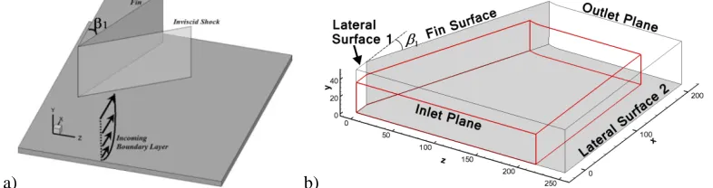
The 3D SWTBLI studied here is set to be at the same flow condition as the experiment of Schülein[10], in which the incoming Mach number is 5 and the deflection angle of the fin is 𝛽₁= 23°. The flow configuration and its computational model are sketched in Figure 1.

a) b)

Figure 1 Sketch maps of the: a) flow configuration and b) computation domain. The red line represents the edges of the effective computation domain.

It can be seen from Figure 1.that, the computational domain in the present study only contains the compression side of the fin, where the 3D SWTBLI happens, and the other side of the fin is discarded to simplify the simulation, like what most numerical simulations in literatures did[12].

The reference length of the simulation is 1 mm and other reference parameters are those of the incoming free-stream flow. The origin of the coordinates is at the leading edge of the fin. The inlet plane is posited at 𝑥=−20mm and is normal to the main flow direction. The outlet plane is beyond 𝑥= 206mm, the spanwise extent of the domain is𝑧< 250mm, and the wall normal size of the domain is 𝑦= 50 mm. Due the employment of the sponge layer in all the three direction, the size of the effective domain, which is marked with red line in Figure 1 b), is (−20, 184.5) × (0, 35) × (0, 215). Considering the nominal boundary layer thickness of the incoming flow𝛿₀ is about 3.8 mm, the size of the domain is about(−5.3𝛿₀, 18.6𝛿₀) × (0, 9.2𝛿₀) × (0, 56.6𝛿₀). The present computational domain is similar with that of the experimental measurement of Schulein[10], and the RANS study of Salin et al. [15], which is convenient for direct comparisons.

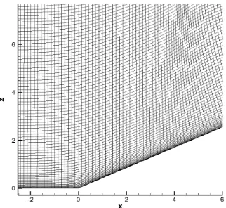
Figure 2 Distributions of the mesh points in the corner region.

B. Numerical Strategy

The Euler terms of the NS equations are solved by using the newly developed seventh-order low-dissipation monotonicity-preserving (MP7-LD) scheme[ 20, 21], which is optimized from the original monotonicity-preserving (MP) scheme of Suresh and Huynh错误!未找到引用源。 by reducing both the linear dissipation and nonlinear error, which has been successfully used in DNS and LES of 2D SWTBLI[22,23]. It was proved that[20], the MP-LD scheme has the same ability as the original MP scheme in capturing shock waves but a better performance in resolving small-scale turbulent fluctuations.

The diffusion terms are solved by using the sixth-order compact central scheme错误!未找到引用源。, which is given as, 1

3𝑓𝑗−1′ +𝑓𝑗′+ 1

3𝑓𝑗+1′ =�𝑓𝑗+2− 𝑓𝑗−2�⁄36+ 7�𝑓𝑗+1− 𝑓𝑗−1�⁄9 (26) The primitive variables𝑢_𝑖 and 𝑇 are firstly differentiated, and the stress tensor is formed at each node. The viscous terms are then computed by another application of Eq. (26). This method is more efficient than the directly calculating second-derivatives, although the later method can be more numerically stable.

The metric of the coordinate transformation is also calculated by using Eq. (26), in the conservative form to preserve the metric cancellation property[24,25], as follows,

⎩ ⎪ ⎪ ⎨ ⎪ ⎪ ⎧𝜉𝑥𝑖=

1

2���𝑥𝑗�𝜂𝑥𝑘�_𝜁+�(𝑥𝑘)𝜂𝑥𝑗�𝜁− ��𝑥𝑗�𝜁𝑥𝑘�_𝜂− �(𝑥𝑘)𝜁𝑥𝑗�𝜂�

𝜂𝑥𝑖 =

1

2���𝑥𝑗�𝜁𝑥𝑘�_𝜉+�(𝑥𝑘)𝜁𝑥𝑗�𝜉− ��𝑥𝑗�𝜉𝑥𝑘�_𝜁− �(𝑥𝑘)𝜉𝑥𝑗�𝜁�

𝜁𝑥𝑖 =

1

2���𝑥𝑗�𝜉𝑥𝑘�_𝜂+�(𝑥𝑘)𝜉𝑥𝑗�𝜂− ��𝑥𝑗�𝜂𝑥𝑘�_𝜉− �(𝑥𝑘)𝜂𝑥𝑗�𝜉�

(27)

After all the spatial terms are solved, the residual terms 𝑅(𝑸) is integrated in time by using the explicit three-step third-order TVD Runge-Kutta scheme错误!未找到引用源。, which is given as,

⎩ ⎨

⎧ 𝑸(1)=𝑸𝑛+∆𝑡𝑅(𝑸𝑛) 𝑸(2)₌3

4𝑸𝑛+ 1 4𝑸(1)+

1

4∆𝑡𝑅�𝑸(1)�

𝑸𝑛+1₌1

3𝑸𝑛+ 2 3𝑸(2)+

2

3∆𝑡𝑅�𝑸(2)�

(28)

At the surfaces of the bottom wall and fin, as shown in Figure 1 b), the isothermal no-slip condition with wall temperature 𝑇_𝑊= 4.39𝑇₀ and adiabatic no-slip condition are used, respectively. The pressure gradient in the wall normal direction is set to be zero.

The boundaries of outlet plane, upper surface and lateral surface 1 in Figure 1 b), are treated with perfectly non-reflective boundary condition, in which all the flow variables at the boundaries are extrapolated from the inside of the domain. To reduce the influences of generated numerical errors at the boundaries, these boundaries are posited far from the effective region by using sponge layers with stretched meshes, and the low-order spatial filter错误!未找到引用

源。

, as shown in Eq. (29), is used to further remove high wavenumber errors in sponge layers.

𝑓̂(𝜉,𝜂,𝜁) =𝑓(𝜉,𝜂,𝜁)− 𝜒 �_𝑙𝑚𝑙𝑠�2{0.5𝑓(𝜉,𝜂,𝜁)−0.25[𝑓(𝜉 −1,𝜂,𝜁) +𝑓(𝜉+ 1,𝜂,𝜁) +𝑓(𝜉,𝜂 −1,𝜁) + 𝑓(𝜉,𝜂+ 1,𝜁) + 𝑓(𝜉,𝜂,𝜁 −1) +𝑓(𝜉,𝜂,𝜁+ 1)]} (29)

Here, 𝑓̂ is filtered variable, 𝑙𝑚 is the length of the sponge layer and 𝑙𝑠 is the distance of the present point to the beginning of the sponge layer. 𝜒 is the filter coefficient, which is set as 0.05, according to reference[错误!未定义书签。].

At the lateral surface 2, where the turbulent flow is truncated, instead of using the conventional periodical boundary condition in 2D simulations, the free-slip boundary condition is applied here. Therefore, 𝑤= 0 and the derivatives of other primitive variables𝑢_𝑖 and 𝑇 are set to be 0 at this boundary. According to our test (not shown here), the influence of this method is small and both flow statistics and main turbulent structures can be preserved. Moreover, the flow can be recovered to the state of equilibrium in the spanwise extent less than 0.1δ.

At the inlet plane, where the flow should be a fully developed turbulent boundary layer, the widely used rescale and reintroduce method[26,27] can hardly be used, due to the lack of the statistically homogeneous direction in the 3D simulation. The synthetic turbulent fluctuations[28,29,30] can be a choice here, however, a transitional region of at least 15 boundary layer thickness in the streamwise is needed before the turbulence can be fully developed. This problem can be very serious here, since a very wide spanwise with large numbers of mesh points is used in the present flow case, therefore, the extended of computational domain in the x direction will cause a great increase of total mesh points.

As an alternative, the present research conducts another independent LES of a flat-plate turbulent boundary layer at Mach=5 with homogeneous spanwise direction, and a time series of flow slices at the particular streamwise section is extracted and saved. The laminar inflow condition is used in the flat-plate boundary layer simulation and the wall blowing and suction, which is similar with that of Rai and Moin[31], is used to trigger the boundary layer transition. Then, these flow slices are introduced to the main LES from the inlet plane with the supersonic inflow condition. This method has three advantages, 1. the turbulence can be fully developed immediately downstream the inlet plane, 2. it’s very convenient to control the boundary layer parameters with the selection of the extracting position, 3. these flow slices can be used in other simulations with the same inflow condition but difference domain sizes or deflection angle.

Since the spanwise size of the main LES is much larger than that of the flat-plate boundary layer. The extracted slices will be replicated and shifted in the spanwise direction.

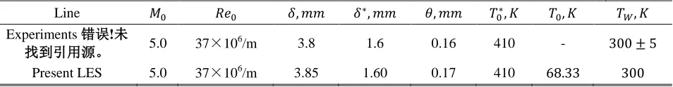
The inflow boundary layer parameters and the comparison with the experiment of Schülein[10] at 20 mm upstream of the leading edge of the fin are given in Table 1.

Table 1 Incoming Boundary Layer Parameter

Line 𝑀₀ 𝑅𝑒₀ 𝛿,𝑚𝑚 𝛿∗,𝑚𝑚 𝜃,𝑚𝑚 𝑇₀∗,𝐾 𝑇₀,𝐾 𝑇_𝑊,𝐾

Experiments 错误!未

找到引用源。 5.0 37×10

6

/m 3.8 1.6 0.16 410 - 300 ± 5

Present LES 5.0 37×106/m 3.85 1.60 0.17 410 68.33 300

IV. Results and Discussions

The time step of the LES is Δ𝑡= 1.5 × 10−2 𝑙₀⁄𝑢₀, which is Δ𝑡+= 9.8 × 10−2 in the wall viscous scale. The simulation persists to 𝑡=1648.5𝑙₀⁄𝑢₀, and 486 instantaneous flow samples are saved every 300 steps for analysis after the simulation is statistically stationary. The Favre statistical averaging is used in the statistics of flow, which is defined as,

〈𝑓̃〉=〈𝜌𝑓〉 〈𝜌〉⁄ (30)

where, 〈 〉 denotes the statistical averaging, which is time and spanwise averaging in the 2D simulation and only time averaging in the 3D simulation. The fluctuation can be got as,

𝑓′′_{=𝑓 − 〈𝑓̃〉 (31)}

𝑓′_{=𝑓 − 〈𝑓〉 (32)}

A. Validation

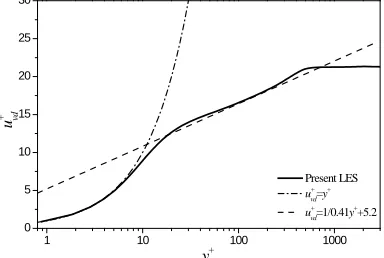
The distribution of the Van Driest transformed mean streamwise velocity 𝑢_𝑣𝑑, at the x=-2 mm is reported in Figure 3. 𝑢_𝑣𝑑 is defined as,

𝑢𝑣𝑑=∫ 〈𝜌〉 〈𝜌₀〈𝑢〉 ⁄ 𝑊〉𝑑〈𝑢〉 (33)

Because the mesh is non-uniform in the spanwise, the averaged is conducted as, 〈𝑢〉=∫ 𝑢𝑑𝑧

𝑧𝑒 0

𝑧𝑒 , where 𝑧𝑒 is the

edge of the effective computation domain in the spanwise. From Figure 3, we can see a good agreement between the present LES results and the classic law of wall in both the linear layer and log layer.

Consistent with Morkovin’s hypothesis, the density-scaled turbulence intensity 𝑢_{𝑖𝑅𝑀𝑆}+ , which is defined as,

𝑢𝑖𝑅𝑀𝑆=�_〈𝜌〈𝜌〉_𝑊〉〈𝑢𝑖′𝑢𝑖′〉 (34)

is reported in Figure 4 in inner a) and outer b) coordinates. According Figure 4, the results of the present LES in the undisturbed boundary layer match well with incompressible DNS data (Spalart[32] and Wu & Moin[33]), compressible DNS at Mach=1.3 (Pirozzoli et al. [34]), as well as low-speed boundary-layer experiments (Purtell et al. [35] and Erm & Joubert[ 36 ]), in both the near-wall region and outer layer of the boundary layer, which indicates that the Morkovin’s hypothesis is still applicable at Mach=5.

1 10 100 1000

0 5 10 15 20 25 30

Present LES

u+ vd=y

+

u+ vd=1/0.41y

+ +5.2

u

+ vd

y+

0 10 20 30 40 50 60 70 80 90 100 0.0 0.3 0.6 0.9 1.2 1.5 1.8 2.1 2.4 2.7 3.0 V el oc ity F luc tuat ion y+ u+ RMS

w+_RMS

v+ RMS

Present LES Purtell et al., 1981 Spalart, 1981 Wu and Moin, 2009 Pirozzoli et al, 2010

0.00 0.25 0.50 0.75 1.00 1.25 1.50 0.0 0.3 0.6 0.9 1.2 1.5 1.8 2.1 2.4 2.7

3.0 Present LES

Purtell et al., 1981 Erm & Joubert, 1991 Wu and Moin, 2009 Pirozzoli, et al., 2010

V el oc ity F luc tuat ion y/δ u+ RMS w+ RMS

v+_RMS

a) b)

Figure 4 Density scaled turbulence fluctuations in: a) inner scaling and b) outer scale at x=-2 mm

The flow statistics in the undistributed boundary layer upstream the leading edge of the fin is in good agreements with experiments and theory, which validates the accuracy of the present LES, at least in the equilibrium region. And it also validates the applicability of the free-slip boundary condition at the lateral surface 2 as well as the inflow turbulence generation technology at the inlet plane.

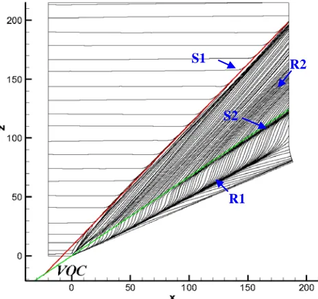
The mean skin-friction-line at the bottom wall is shown in Figure 5. With the Critical Point Theory (CPT), the 3D flow separation and attachment can be recognized by the convergence and divergence of the skin-friction-lines receptively. From Figure 5, we can clearly see the main flow separation line S1, attachment line R1 and the secondary separation line S2. The following analysis of the wall pressure distribution also indicates the appearance of the secondary reattachment. Therefore, the pattern of wall streamlines of present case is coincident with that of the regime VI in the regime map of Zheltovodov and Knight[16] reproduced in Figure 6 at same similar Mach number and deflection angle.

Figure 5 Mean skin-friction-line at the bottom wall. The red and green lines present S1 and the inviscid shock.

S1

R1 S2

Figure 6 The boundaries of swept-shock-wave/turbulent-boundary-layer interaction regimes and corresponding surface flow pattern. This figure is reproduced from Ref [16].

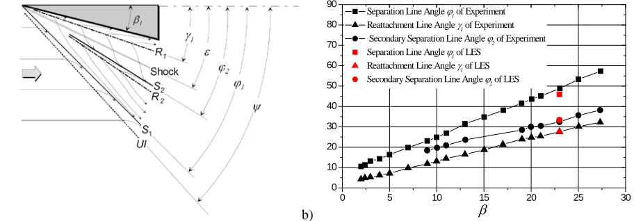
The comparisons of the angle of the separation line S1, the reattachment R1 and the secondary separation line S2 between the experiment measurements of Schülein and Zheltovodov[37] and present LES are shown in Figure 7. The agreement between the present LES and experiments is satisfactory.

a) b)

0 5 10 15 20 25 30

0 10 20 30 40 50 60 70 80 90

Separation Line Angle ϕ₁ of Experiment Reattachment Line Angle γ

1 of Experiment

Secondary Separation Line Angle ϕ

2 of Experiment

Separation Line Angle ϕ₁ of LES Reattachment Line Angle γ

1 of LES

Secondary Separation Line Angle ϕ

2 of LES

β

Figure 7 The definition of the angles of the separation and reattachment lines (a) and their distributions in the experiment and present LES (b)

The wall pressure distributions at the cross sections of x=83mm, x=93mm, x=123mm, x=153mm and x=183mm are compared with the measurements of of Schülein[10] as well as Schülein and Zheltovodov[37] in Figure 8 (a), from which we can see the good agreement of the LES prediction and the experimental measurements. The separation and reattachment lines can also be reflected from the local peaks of the wall pressure distribution. Although the secondary reattachment R2 is not so evidently from the skin-friction-line topology, it can be seen clearly on the wall pressure distribution at x=183 mm.

a)

0.4 0.6 0.8 1.0 1.2 1.4 1.6

-3 0 3 5 8 10 13 15 18 20 S1

LES Results at x=83 mm LES Results at x=93 mm LES Results at x=123 mm LES Results at x=153 mm LES Results at x=183 mm Experiment Measure at x=83 mm Experiment Measure at x=93 mm Experiment Measure at x=123 mm Experiment Measure at x=153 mm Experiment Measure at x=183 mm

pW / p∞ z/x R1 S2 R2 b)

0.4 0.6 0.8 1.0 1.2 1.4 1.6

0.000 0.005 0.010 0.015 0.020 0.025

LES Result at x=82 mm

LES Result at x=122 mm

LES Result at x=162 mm

LES Result at x=182 mm

Experiment Measure at x=182 mm

Experiment Measure at x=162 mm

Experiment Measure at x=122 mm

Experiment Measure at x=82 mm

C

f

z/x

Figure 8 The distributions of wall pressure (a) and skin friction coefficient (b) at several x-slices

B. Virtual Conical Origin Coordinates

According to previous researches[12, 39- 44], the nature of the flow-field are quasi-conical except for an initial region in the vicinity of the fin’s leading-edge. Beyond this initial region, flow topological features appear to emanate from a single point, which is named the “Virtual Conical Origin” (VCO) and the Spherical coordinate system (𝑅,𝛽,𝜑) is an appropriate coordinate frame to study these flows (see [42]). In the present study, VOS is determined as the intersection of the primary separation line S1 and the extension of inviscid shock-wave trance, as show in Figure 5. The position of VCO is at (-22.57mm, 0mm, -14.91mm). The VCO coordinate system is sketched in Figure 9. In Figure 9 (b), another coordinates system (𝑥₁,𝑦₁), with the origin at the leading (𝑥,𝑦,𝑧) = (0,0,0) and the direction of 𝑥₁ parallel to the surface of the fin.

a) b)

Figure 9 Sketch map of the VCO coordinate system. b) is the projection of a) to the bottom wall The Cartesian velocity vector (𝑢,𝑣,𝑤) can be projected to the VCO coordinates as �𝑢_𝑅,𝑢_𝛽,𝑢_𝜑�, with the following formulas,

𝑢𝛽=−𝑢sin(𝛽) +𝑤cos(𝛽), (36)

𝑢𝜑=−𝑢sin(𝜑)cos(𝛽) +𝑣cos(𝜑) +𝑤sin(𝜑)sin(𝛽), (37)

Therefore, the normal Reynolds stress components in the VCO coordinates can be expressed as,

〈𝑢𝑅′′𝑢𝑅′′〉=〈𝑢′′𝑢′′〉cos2(𝜑)cos2(𝛽) +〈𝑣′′𝑣′′〉sin2(𝜑) +〈𝑤′′𝑤′′〉cos2(𝜑)sin2(𝛽) + 2〈𝑢′′𝑣′′〉cos(𝜑)sin(𝜑)cos(𝛽) + 2〈𝑢′′_𝑤′′_〉cos2_{(𝜑)cos(𝛽)sin(𝛽) + 2〈𝑣}′′_𝑤′′_{〉sin(𝜑)cos(𝜑)sin(𝛽),}

(38)

〈𝑢𝛽′′𝑢𝛽′′〉=〈𝑢′′𝑢′′〉sin2(𝛽) +〈𝑤′′𝑤′′〉cos2(𝛽)−2 〈𝑢′′𝑤′′〉cos(𝛽)sin(𝛽), (39)

〈𝑢𝜑′′𝑢𝜑′′〉=〈𝑢′′𝑢′′〉sin2(𝜑)cos2(𝛽) +〈𝑣′′𝑣′′〉cos2(𝜑) +〈𝑤′′𝑤′′〉sin2(𝜑)sin2(𝛽)−2〈𝑢′′𝑣′′〉cos(𝜑)sin(𝜑)cos(𝛽)

−2〈𝑢′′_𝑤′′_〉sin2_{(𝜑)cos(𝛽)sin(𝛽)−2〈𝑣}′′_𝑤′′_{〉sin(𝜑)cos(𝜑)sin(𝛽),} (40)

The conical-cross Mach number 𝑀_𝑛 can be defined as

𝑀𝑛=�𝑢𝛽2+𝑢𝜑2�𝐶, (41)

where 𝐶 is the local speed of sound. C. Shock Structures

The numerical schlieren 𝑟𝑛𝑠 and pressure gradient magnitude |∇𝑝| is used to analyze the shock structures. 𝑟𝑛𝑠 is calculated according to the formula,

𝑟𝑛𝑠=𝑐1𝑒−𝑐2(|∇𝜌|−|∇𝜌|𝑚𝑖𝑛) (|⁄ ∇𝜌|−|∇𝜌|𝑚𝑎𝑥) (42)

, where |∇𝜌| =�𝜕𝜌 𝜕𝑥𝑖

𝜕𝜌

𝜕𝑥𝑖, 𝑐1= 0.8 and 𝑐2= 10.

|∇𝑝| is defined as |∇𝑝| =�𝜕𝑝 𝜕𝑥𝑖

𝜕𝑝

𝜕𝑥𝑖 and is normalized with 𝑝∞⁄𝛿0, where 𝛿0 is the nominal boundary layer

thickness of the incoming flow.

The mean location of the normal shock can be reflected in the map of the mean density schlieren and pressure gradient magnitude |∇〈𝑝〉| in Figure 11

a)

b)

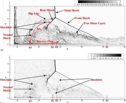
Figure 10 Instantaneous numerical schlieren (a) and pressure gradient field (b) on the 3-D spherical arc section at 𝑹=𝟐𝟐𝟔.𝟑𝐦𝐦

The flow structure here is similar with that described by Alvi and Settles[47,48]at the similar flow regime. After S1, the flow is deflected away from the wall and a free shear layer is then generated, which is similar with that in the two dimensional SWTBLI[34]. From the density schlieren, the turbulent structures can also be investigated. Firstly, we can see some large-scale structures in the free shear layer and around the slip line, which is attributed to the Kelvin–Helmholtz instability. In the near-wall region beneath the main separation bubble, some small-scale structures attached to the wall can be seen. Therefore, unlike the 2D flow separation region, in which the flow is less fluctuant and organized, the reverse flow inside the 3D separation bubble has energetic turbulent fluctuations.

Front Shock Main Shock

Rear Shock Slip Line

Free Shear Layer

Jet Shocklets

Normal Shock

Shocklets

Normal Shock

Figure 11 Mean numerical schlieren (a) and pressure gradient field (b) on the 3-D spherical arc section at

𝑹=𝟐𝟐𝟔.𝟑𝐦𝐦

The instantaneous 3D structure of the shock wave is visualized by using the iso-surface of |∇𝑝| in Figure 12. From the figure, we can see that, the main shock-wave is a two dimensional straight surface. The front shock-wave, however, presents a three dimensional wrinkle face. Near the shock foot, lots of small-scale wrinkle can be seen, and with the increase of the distance to the wall, the scale of the wrinkle becomes larger, which indicates the wrinkle of the shock surface is attributed to the interaction with the incoming turbulent structures. By extending the line of triple point and the line of the shock foot, we can see that, the two lines intersect at the VCO, which validates the quasi-conical characteristic of the shock surface.

Normal Shock

Figure 12 Instantaneous shock surface visualized by using the iso-surface of the pressure gradient magnitude |𝛁𝒑| =𝟓 𝒑∞⁄𝜹𝟎

D. Streamlines

The skin-friction-line in the region near the leading edge is examined in Figure 13. Saddle and focus points can be identified upstream and downstream the leading edge, respectively. Zheltovodov[39] also reported the existence of saddle-point located on the separation line S1 upstream of the fin leading edge. However, the focus point has never been reported before. It can be seen from Figure 13 that, almost all the streamlines in the interaction region are emitted from this focus. Some of these streamlines go upstream and merge with the incoming streamlines to converge the separation line S1, and some of streamlines go downstream and form the attachment line R1. There are also some streamlines going towards the fin and ends at the surface.

a) b)

Figure 13 Mean skin-friction-line near the leading edge and the focus in a) is zoomed out in b).

surface of the fin can also be found in the experimental oil-flow visualization by Zheltovodov[39] as described by Zheltovodov and Knight[16]) in the same flow regime (Mach=4, β=30.5°), which indicates the existence of a longitudinal corner separation vortex.

a)

b)

Figure 14 Mean skin-friction-line at the surface of the fin. The near-wall region is zoomed out in b)

The streamlines �𝑢_𝛽,𝑢_𝜑� on the 3-D spherical arc section at R=226.3 mm are presented in Figure 15. Unlike the closed configuration of the streamlines in the 2D separation bubble, the streamlines in Figure 15 spiral around two focuses into which they disappear, therefore, present the 3D characteristic of the present flow separation. The two focuses are respectively the main separation vortex core and the corner vortex core.

Figure 15 Mean streamlines �𝒖_𝜷,𝒖_𝝋� on the 3-D spherical arc section at 𝑹=𝟐𝟐𝟔.𝟑𝐦𝐦.

The streamline-surfaces are shown in Figure 16, from which we can see that, the streamlines lift through the separation line and fall off near the attachment line, which can be explained with the theory of Lighthill[49]. The streamlines originating from different values of y are shown in Figure 17. It can be seen that, the streamlines from different heights presents different structures. The streamlines originating from the near-wall region (Figure 17 a)

Main Separation Vortex Core Corner

presents a spiral structure around the separation vortex core. With the increase of the origination position (Figure 17 b), the streamlines directly enter the reversal flow, rather than through the vortex core. Further increase the height (Figure 17 c), some of the streamlines go into the corner region, which indicates the existence of the corner vortex. The streamlines out of the boundary layer will not become the reversal flow; instead, they impinge to the mean attachment line R1 and move towards the surface of the fin.

Figure 16 Streamline-surfaces of the mean flow. The color stands for 〈𝒖〉

a) b)

c) d)

The streamlines in the corner region are zoomed in Figure 18, in which the helical streamlines indicating the existence of the corner vortex can be clearly seen. The corner vortex originates near the leading edge of the fin’s surface. Further downstream, the fluid in the corner vortex will have larger speed, which can be attributed to the strong sweeping events caused by the flow impinging towards the corner region.

Figure 18 Streamlines in the corner region, with the color of the mean value of u E. Mean Flow Field

The mean density field normalized with its incoming value on the section at R=226.3 mm is demonstrated in Figure 19. The experimental results of Hsu and Settle[ 50 ]at Mach=4 with 21° deflection angel is shown for qualitative comparison. The main flow feather including the shock structures, the separation vortex, and the separation shear layer are consistent with the experimental observation. From the figure, we can see the free shear layer rolls up tightly to form a distinct vortex core.

a)

1

2 3

b)

Figure 19 Distributions of: a) the normalized mean density on the section at 𝑹=𝟐𝟐𝟔.𝟑𝐦𝐦, and b) experimental results of Hsu and Settles 0 at Mach=4, β=21°,. 1, 2, 3, and 4 in the figure stand for the main

shock, separation shock, rear shock, and main vortex core, respectively.

The mean stagnation pressure, static pressure and conical-cross Mach number 𝑀_𝑛 are presented in Figure 20, from which, we can see the jet flow with high level of stagnation pressure rolling around the vortex core. The jet is supersonic initially and gets accelerated during the expansion process. The supersonic jet is terminated by the interaction with the normal shock (can be seen in Figure 11) and it further penetrates underneath the main vortex into the near-wall separation region and gets accelerated to supersonic (Figure 20 c) again. Near the impinging location R1, the density and pressure get high (Figure 20 b), and the high pressure drives the flow to the fin’s surface and its reverse direction. Near the secondary separation line S2, the adverse pressure gradient can be seen, which should be attributed to the shocklets and the normal shock (as shown in Figure 10 b) in this region. The adverse pressure gradient should be the reason for the secondary flow separation. After S2, the reversal jet is detached from the wall, just like the main flow separation.

The penetration of jet brings high energy fluid to the near-wall reverse flow and is responsible for the energetic turbulence in this the reverse flow layer. Such mechanism is missing in a 2D SWTBLI, therefore, the reverse flow in a 2D flow separation is usually quiet and less organized. The mean kinetic energy 1

a)

b)

c)

Figure 20 Distributions of: a) the stagnation pressure, b) the static pressure, and c) the conical-cross Mach number𝑴_𝒏 , on the section at 𝑹=𝟐𝟐𝟔.𝟑𝐦𝐦. The black thin line in c) denotes the contour with 𝑴_𝒏=𝟏.

The mean shear strength, which can be measured with the vorticity magnitude as

𝜔𝑛=�〈𝜔𝑥〉2+〈𝜔𝑦〉2+〈𝜔𝑧〉2, is shown in Figure 21, from which we can see that, regardless the near-wall region, where the shear strength is always large, the strong shear region includes the free-shear layer caused by the main flow separation and the slip line. The shear strength in the center of the jet is low, which can be seen as a common characteristic of the jet flow. The shear strength is strong in the begin parts of the main flow separation and the slip line. With the further develop of the free shear layer, the shear strength decreases due to the diffusion nature of the mixing layer.

Figure 21 Distributions of the mean vorticity strength 𝝎_𝒏 on the section at 𝑹=𝟐𝟐𝟔.𝟑𝐦𝐦. 𝝎_𝒏 is normalized with 𝒖_𝟎⁄𝜹_𝟎.

F. Instantaneous Flow Field

To explore the turbulence characteristics, the instantaneous flow field is analyzed in this section. Figure 22 demonstrates the instantaneous streamwise velocity fluctuations 𝑢_𝑠′′ in the near-wall 𝑥 − 𝑧 plane at 𝑦= 0.085mm (𝑦+= 10 at the inlet plane). 𝑢_𝑠′′ is defined as,

𝑢𝑠′′=𝑢�⃗′′∙ 𝑛�⃗, (36)

where 𝑢�⃗′′= (𝑢′′,𝑣′′,𝑤′′)𝑇 is the vector of the velocity fluctuation and 𝑛�⃗=〈𝑢�⃗〉⁄|〈𝑢�⃗〉| is the unit vector of the mean flow.

a) b)

c)

Figure 22 Instantaneous fields of 𝒖_𝒔′′ at 𝒚=𝟎.𝟎𝟖𝟓𝐦𝐦. The squared regions in a) are zoomed in b) and c). The red, blue and green lines represent the mean separation line S1, reattachment line R1 and the secondary

line S2.

It can be inferred that, the regeneration of the wall turbulence is caused by the reattached reverse flow. As represented in Figure 20, the jet flow originated from the external flow, brings fluids with high kinetic energy to the near-wall region and the pressure gradient further drives high energy fluids to the near-wall region of the separation zone as the reverse flow. Consequently, the near-wall flow has strong kinetic energy and fluctuations and promotes the transition of the flow to turbulent in a very short distance. The transiting process can be seen in Figure 22 (b), in which a small region around R1 has less organized structures. This region in the location on which the jet impinges, as shown in Figure 15, therefore, the turbulent is not organized yet. At both sides of R1, the streaky structures are regenerated in a short distance, indicating the regeneration of the near-wall turbulence.

Near S2, we can see the streaks are distorted and activated by APG again, which is similar with the process of the main flow separation. But the flow structures in the secondary separation don’t show much variation.

fluctuation at y=1.32 mm is weaker and has larger length scale than those in the near-wall region (as shown in Figure 22 a), which can be attributed to the ejection of low-momentum fluid by the large-scale horseshoe vortex head in the boundary layer. Near the front shock, the fluctuations are amplified, which is attributed to the unsteady movement of the shock-wave. In the core of the reverse jet, the flow is less fluctuant and less organized. For the slice at y=8.15mm (about 2δ0), the flow upstream the shock-wave is almost inviscid, however, in the interaction zone, strong fluctuations can be seen. These fluctuations are generated by the free shear of the detached flow layer of the main flow separation.

a) b)

Figure 23 Instantaneous fields of 𝒖_𝒔′′at a) y=1.32 mm and b) y= 8.15 mm.

a)

b) c) d)

Figure 24 Instantaneous 𝒖_𝑹′′ on the section at 𝑹=𝟐𝟐𝟔.𝟑𝐦𝐦. b), c) and d) are the zoomed picture of local flow structures in a). The arrow stands for the 2D vector of �𝒖_𝜷′′,𝒖_𝝋′′�. 1 indicates the undisturbed wall

turbulent structure, 2 indicates for the large scale vortex in the shear layer, 3 indicates the large-scale structures in the jet, 4 indicates the regenerated wall turbulent structures, 5 indicates the low-turbulent zone.

The vorticity fluctuation in the R direction 𝜔_𝑅′′ and the swirling strength 𝜆_𝑐𝑖[54]on the section of 𝑅= 226.3mm are present in Figure 25, in which 𝜔_𝑅′′ and 𝜆_𝑐𝑖 are normalized with 𝑢₀⁄𝛿₀ and (𝑢₀⁄𝛿₀)2, respectively. Since the vorticity and swirling strength are closely related to the turbulent structures, the above mentioned five zones (as marked in Figure 25 a), are more distinguishable in Figure 25.

The structures in the zone 1 are the combination of small-scale strong fluctuations in the near-wall region and large-scale weaker fluctuations in the outer region. The turbulence in zone 2 is also very strong, and these fluctuations are weakened with the diffusion of the free-shear layer. The zone 3 only occupies only a slim region, in which the transition of the shear layer by Kelvin–Helmholtz instability can be seen. The zone 4 is a thin layer attached to the wall, but the fluctuations in it are strong. The zone 5 present a gap between zone 2, zone 3 and zone 5, and the space of the gap become larger with the further development of the shear layer, due to the quasi-conical property of the flow. The transition process can be seen in the zone 3. The intensity and the length scale of the structures in this zone increase with the development of the jet flow, and finally these structures enter the core region and the reverse flow after the impingement of the jet. Besides the 5 zones, the turbulence in the corner region also presents complex property, due to the complex flow mechanism in this region.

4 2

3 4

1 2

3

a)

b)

Figure 25 Instantaneous field of vorticity fluctuation 𝝎_𝑹′′ a) and 𝝀_𝒄𝒊 b) on the section at 𝑹=𝟐𝟐𝟔.𝟑𝐦𝐦. The iso-surface of 𝜆_𝑐𝑖 is used to visualize the spatial distribution of turbulent coherent structures in Figure 26. Because of the data is too big for the 3D flow visualization, only the upstream half of the domain is presented. Firstly, the horseshow vortex in the zone 1 can be clearly identified in Figure 26. In the interaction zone, the most noticeable phenomena is the great amplification of the turbulence coherent structures in the zone 2, since the zone 2 occupies the most place of the interaction region. The gap in the zone 3 and zone 5 indicates the turbulence is weak in these two regions. The wall-turbulence in zone 4 can be seen in Figure 26 (b), where only the near-wall part is shown. In the transition region between zone 1 and zone 2, the turbulence is amplified the most, because of the strong ADG in this place.

a) b)

1 1

2 3

4

Figure 26 Turbulence coherent structures visualized using iso-surface of 𝝀_𝒄𝒊 equaling to 0.5% of its global maximum, rendered with the instantaneous u. b) only demonstrates the region of 𝒚+<𝟓𝟎. Only the

upstream part of the domain is presented. G. Turbulence Statistics

The turbulent kinetic energy (TKE) 𝐾=1

2�〈𝑢′′𝑢′′〉� +〈𝑣′′𝑣′′〉� +〈𝑤′′𝑤′′〉� � on the section of 𝑅= 226.3mm is presented in Figure 27. Consistent with the previous analysis, TKE presents high values in the zone 2. The zone 3 also has a certain level of TKE and the turbulent energy spreads outwards with the transition of the jet flow. In the zone 5, the level of TKE is lower than its circumstance. Near S2, the increase of TKE and the thickening of the near-wall shear-layer can be seen, which can be seen more clearly in the zoomed figure Figure 27 (b). The amplification mechanism is also the activation of turbulence by the adverse pressure gradient, which is similar with that of the amplification of turbulence at S1. However, the amplification of turbulence at S2 is only restrained in a limited region, therefore, no large-scale separation region and detached free-shear layer can be observed. Passing through S2, the TKE decreases to the level before the secondary separation.

a)

b)

Figure 27 Turbulent kinetic energy on the section at 𝑹=𝟐𝟐𝟔.𝟑𝐦𝐦, normalized with the square of the wall friction velocity 𝒖_𝝉𝟐 at the inlet.

Figure 28 Pressure fluctuation intensity〈𝒑′𝒑′〉 𝒑⁄ _∞𝟐, on the section at 𝑹=𝟐𝟐𝟔.𝟑𝐦𝐦.

The further investigation of compressibility is conducted by check the instantaneous pressure fluctuant field

𝑝′ 𝑝⁄ ∞ and the velocity divergence ∇ ∙ 𝑢�⃗ are shown in Figure 29. Large values of 𝑝′ and negative values of ∇ ∙ 𝑢�⃗ can be identified in the regions with high levels of pressure fluctuations in Figure 28. Near R1, 𝑝′ shown some strong fluctuation, however, no negative values of ∇ ∙ 𝑢�⃗ can be seen in that region. Therefore, the high level of pressure fluctuations around the mean reattachment region is not caused by the compressibility. Low levels of the ∇ ∙ 𝑢�⃗ and 𝑝′ can be seen in the acceleration part of the reverse flow, which can be explained by the reduction of fluctuant energy in an accelerated flow. Near S2, negative ∇ ∙ 𝑢�⃗ and high values of 𝑝′ can be seen, which indicates the existence of shocklets or a normal shock, which terminates the supersonic jet and causes the secondary flow separation.

The acoustic waves can be identified in the free-stream region left the main shock and rear shock. The acoustic waves are radiated from the jet flow and propagate towards the top left corner. The acoustic waves cann’t penetrate the main shock-wave and the front shock-wave, therefore, the flow in the undisturbed region has a very low level of pressure fluctuation, therefore is quiet.

a)

b)

Figure 29 Flow fields of a) pressure fluctuation 𝒑′ 𝒑⁄ _∞ and b) velocity divergence𝛁 ∙ 𝒖��⃗, on the section at

𝑹=𝟐𝟐𝟔.𝟑𝐦𝐦. 𝛁 ∙ 𝒖��⃗ is normalized with 𝒖_𝟎⁄𝜹_𝟎.

V. Concluding Remarks

The 3D SWTBLI in the flow passing a single-fin at Mach 5 is investigated in the present paper by using LES. The performed LES has demonstrated very good agreement with experimental data in the mean flowfield structure, surface pressure as well as surface flow pattern. However, significant underpediction in surface skin-friction maximum in the vicinity of the reattachment line (R1) is observed. The specification of a reason of such discrepancy as well as analysis of surface heat transfer prediction is important and will be analyzed at the next stage of research. The LES data are then analyzed to investigate the flow property and the turbulence characteristic. Some conclusions are reached,

1. The λ-shock system is formed in the 3D SWTBLI and the shock waves are unsteady. The wrinkling of the front shock surface can be seen, and the scale of wrinkles increases with the distance to the wall, which is caused by the interaction with large-scale turbulent structures in the incoming flow.

2. By analyzing the mean skin-friction-line with the Critical Point Theory, the flow is separated at the foot of the separation shock and reattached near the corner region. The secondary flow separation and reattachment lines can also be identified, which is consistent with the regime characteristic of Zheltovodov and Knight[16]. Near the leading edge of the fin, a saddle and a focus can be identified upstream and downstream of the leading edge, respectively. All the skin-friction-lines in the interaction zone are emitted from the focus. The streamlines lift at the separation line and fall off near the fin’s surface, which transport the fluid with high energy to the near wall region. In the separation vortex, the streamlines curls around the separation vortex core, and generate the reverse flow beneath the separation vortex. The helical streamlines in the corner region indicates the existence of the corner vortex.

3. A free shear layer with strong mean shear strength and high kinetic energy is generated when flow is detached near the mean separation line. The free shear layer is deflected away from the wall from the separation line and the vortex core is therefore formed. A jet flow originating from the rear shock leg, rolls tightly around the vortex core and impinges to the wall at the mean reattachment line. The supersonic jet penetrates into the reverse flow beneath the separation vortex and brings fluids with high energy to the reverse flow. The supersonic jet is terminated by interaction with a normal shock and then impinges to the bottom wall near the mean reattachment line, inducing high level of pressure there. The high pressure drives the reverse flow to supersonic, which is then terminated by another interaction with a normal shock inside the reverse flow, and causes the secondary flow separation.

4. The great change of turbulence characteristic can be found in the interaction zone. The flow field can be categorized into 5 zones according to the characteristics of turbulent structures. Zone 1 is the undisturbed wall turbulence in the upstream boundary layer. Zone 2 is the separated free shear layer, which contains some large-scale structures with high fluctuant energy. Zone 3 is the slip line, which is also the edge of the jet. The turbulence in this zone is also dominated by the free shear but the flow is still in the process of transition. Zone 4 is the reverse flow, which also characterized by the turbulence, but only restrained in a thin layer attached to the wall. The wall-turbulence is induced by the jet flow, which has strong kinetic energy and large-scale fluctuations. Zone 5 is the low-turbulent zone, which includes the core of jet and the gap between the zone 2 and zone 4.

5. The pressure fluctuations are strong in the region with shocks, which includes the λ-shock system and the normal shocks in the jet and reverse flow. The pressure fluctuations in the jet flow keep high levels, which can be attributed to the complex expansion waves, compression waves and shocklets in the jet. However, the high pressure fluctuations near the mean reattachment line are not caused by the compressibility but by the impinging of the jet on a wall. Strong acoustic waves are generated by the jet and propagate towards the side of the fin.

Acknowledgments

This work is supported by the National Natural Science Foundation of China (51420105008, 11302012, 51136003, 50976010, 51006006), China Postdoctoral Science Foundation, the National Basic Research Program of China (2012CB720205), National Magnetic Confinement Fusion Research Program of China(2012GB102006), the Aeronautical Science Foundation of China (2010ZB51025), the 111 Project (B08009), and the Astronautical Technology Innovation Foundation of China. The computer time for the present study was provided via the UK Turbulence Consortium (EPSRC grant EP/G069581/1) and the simulations were run on the UK High Performance Computing Service ARCHER.

1

Dolling, D. S., “Fifty Years of Shock-Wave/Boundary-Layer Interaction Research: What Next?” AIAA Journal, Vol. 39, No. 8, 2001, pp. 1517–1531.

2

Panov, Y. A., “Interaction of a three-dimensional shock wave with a turbulent boundary layer”, Fluid Dynamics, Vol. 1, No. 4, 1966, pp. 131–133.

3

Settles, G. S., Perkins, J. J., and Bogdonoff, S. M., “Investigation of three-dimensional shock/boundary-layer interaction at swept compression corners,” AIAA Journal, Vol. 18, No. 7, 1980, pp. 779–785.

4

Kubota, H. and Stollery, J. L., “An experimental study of the interaction between a glancing shock wave and a turbulent boundary layer,” Journal of Fluid Mechanics, Vol. 116, 1982, pp. 431–458.

5 _{Settles, G. S. and Bogdonoff, S. M., “Scaling of two- and three-dimensional shock/turbulent boundary-layer interactions at}

compression corners,” AIAA Journal, Vol. 20 No. 6, 1982, pp. 782–789.

6

Dolling, D. S. and Bogdonoff, S. M., “Upstream influence in sharp fin-induced shock wave/turbulent boundary layer interaction,” AIAA Journal, Vol. 21, No. 1, 1983, pp. 143–145.

7

Alvi, F. S., and Settles, G. S., “A physical model of the swept shock/boundary-layer interaction flowfield,” AIAA Journal, Vol. 30, No. 9, 1992, pp. 2252-2258.

8

Zheltovodov, A. A., Maksimov, A. I., and Shevchenko, A. M., “Topology of three-dimensional separation under the conditions of symmetric interaction of crossing shocks and expansion waves with turbulent boundary layer,” Thermophysics and Aeromechanics, 5 (1998), 3, 293–312.

9

Zheltovodov, A. A., “Some advances in research of shock wave turbulent boundary-layer interactions,” 44th AIAA Aerospace Sciences Meeting and Exhibit, 2006, AIAA Paper 2006–0496.

10

Schülein, E., “Skin-Friction and Heat Flux Measurements in Shock/Boundary-Layer Interaction Flows,” AIAA Journal, 2006, Vol. 8, No.44, pp. 1732–1741.

11

Hung, C. M. and MacCormack., R. W. “Numerical solution of three-dimensional shock wave and turbulent boundary-layer interaction,” AIAA Journal, Vol. 16, 1978, pp. 1090–1096.

12

Panaras, A. G., “Numerical Investigation of the High Speed Conical Flow Past a Sharp Fin,” Journal of Fluid Mechanics, Vol. 236, 1992, pp. 607–633.

13

Panaras. A. G., “Calculation of flows characterized by extensive cross-flow separation,” AIAA Journal, Vol. 42, No. 12, 2004, pp. 2474–2481.

14

Knight, D., Gnedin, M., Becht, R., and Zheltovodov, A., “Numerical simulation of crossing shock-wave/turbulent-boundary-layer interaction using a two-equation model of turbulence,” Journal of Fluid Mechanics, Vol. 409, 2000, pp. 121–147.

15 _{Salin, A., Yao, Y. F., Lo, S. H., and Zheltovodov, A. A., “Flow Topology of Symmetric Crossing Shock Wave Boundary}

Layer Interactions,” Proceedings of the 28th International Symposium on Shock Waves, 2012, pp. 425–431.

16

Zheltovodov, A. A. and Knight, D. D., “Ideal-Gas Shock-Wave-Turbulent Boundary-Layer Interactions in Supersonic Flows and their Modeling: Three-Dimensional Interactions,” Shock Wave-Boundary-Layer Interactions, edited by H. Babinsky and J. K. Harvey, Cambridge Aerospace Series, Cambridge University Press, London, 2011, pp. 202–258.

17

Moin, P., Squires, W., Cabot, W., and Lee, S., “A dynamic subgrid-scale model for compressible turbulence and scalar transport,” Physics of Fluids A, Vol. 3, No. 11, 1991, pp. 2746 –2757.

18

Ghosal, S., Lund, T. S., Moin, P., and Akselvoll, K., “A dynamic localization model for large eddy simulation of turbulent flows,” Journal of Fluid Mechanics, Vol. 286, 1995, pp. 229-255.

19

Thomas, P. D., and Middlecoff, J. F., “Direct Control of the Grid Point Distribution in Meshes Generated by Elliptic Equations,” AIAA Journal, Vol.18, No. 6, 1980, pp. 652-656.

20

Fang, J., Li, Z. and Lu, L., “An Optimized Low-Dissipation Monotonicity-Preserving Scheme for Numerical Simulations of High-Speed Turbulent Flows,” Journal of Scientific Computing, Vol. 56, 2013, pp. 67-95.

21

Fang, J., Yao, Y., Li, Z., and Lu, L., “Investigation of low-dissipation monotonicity-preserving scheme for direct numerical simulation of compressible turbulent flows,” Computers & Fluids, Vol. 104, 2014, pp. 55-72.

22

Li, Z. and Jaberi, F. A., “A High-Order Finite Difference Method for Numerical Simulations of Supersonic Turbulent Flows,” Journal for Numerical Methods in Fluids, Vol. 68, No. 6, 2011, pp. 740-766.

23

Jammalamadaka, A., Li, Z. and Jaberi, F. A., “Subgrid-Scale Models for Large-Eddy Simulations of Shock-Boundary-Layer Interactions,” AIAA Journal, Vol. 51, No. 5, 2013, pp. 1174-1188.

24

Thomas, P. D. and Lombard, C. K., “Geometric conservation law and its application to flow computations on moving grids.” AIAA Journal, Vol. 17, No.10, 1979, pp. 1030-1037.

25

Visbal, M. R. and Gaitonde, D. V., “Computation of Aeroacoustic Fields On General Geometries Using Compact Differencing and Filtering Schemes,” 30th AIAA Fluid Dynamics Conference, 1999, AIAA Paper 99-3706.

26

Lund, T. S., Wu, X. and Squires, K. D., “Generation of Turbulent Inflow Data for Spatially-Developing Boundary Layer Simulations,” Journal of Computational Physics, Vol. 140, 1998, pp. 233-258.

27

28

Le, H., Moin, P., and Kim, J., “Direct numerical simulation of turbulent flow over a backward-facing step,” Journal of Fluid Mechanics, Vol. 330, 1997, pp. 349-374.

29

Klein, M., Sadiki, A., Janicka, J., “A Digital Filter Based Generation of Inflow Data for Spatially Developing Direct Numerical or Large Eddy Simulations,” Journal of Computational Physics, Vol. 186, 2003, pp. 652–665. 30

Touber, E. and Sandham, N. D., “Large-Eddy Simulation of Low-Frequency Unsteadiness in a Turbulent Shock-Induced Separation Bubble,” Theoretical and Computational Fluid Dynamics, Vol. 23, 2009, pp. 79-107.

31

Rai, M. M., and Moin, P., “Direct Numerical Simulation of Transition and Turbulence in a Spatially Evolving Boundary Layer,” Journal of Computational Physics, Vol. 109, 1993, pp. 169-192.

32

Spalart, P. R., “Direct Numerical Simulation of a Turbulent Boundary Layer Up to Reθ=1410,” Journal of Fluid Mechanics, Vol. 187, 1988, pp. 61-98.

33

Wu, X., and Moin, P., “Direct Numerical Simulation of Turbulence in a Nominally Zero-Pressure-Gradient Flat-Plate Boundary Layer,” Journal of Fluid Mechanics, Vol. 630, 2009, pp. 5-41.

34

Pirozzoli, S., Bernardini, M., and Grasso, F., “Direct Numerical Simulation of Transonic Shock/Boundary Layer Interaction Under Conditions of Incipient Separation,” Journal of Fluid Mechanics, Vol. 657, 2010, pp. 361-393. 35

Purtell, L. P., Klebanoff, P. S., and Buckley, F. T., “Turbulent Boundary Layer at Low Reynolds Number,” Physics of Fluids, Vol. 24, 1981, pp. 802-811.

36

Erm, L. P., and Joubert, P. N., “Low Reynolds Number Turbulent Boundary Layers,” Journal of Fluid Mechanics, Vol. 230, 1991, pp. 1-44.

37

Schülein, E., and Zheltovodov, A.A., "Documentation of experimental data for hypersonic 3-D shock waves/turbulent boundary layer interaction flows," DLR Gottingen, 2001, IB 223 – 99 A 26.

38

Pasha, A. A. and Sinha, K., “Simulation of three-dimensional shock/boundary-layer interaction in a single-fin configuration,” 11th Annual CFD Symposium. Bangalore, 2009.

39

Zheltovodov, A., “Regimes and properties of three-dimensional separation flows initiated by skewed compression shocks,” Journal of Applied Mechanics and Technical Physics, Vol. 23, No. 3, 1982, pp. 413–418.

40

Alvi, F.S., and Settles, G.S., "Physical Model of the Swept Shock-Wave/Boundary-Layer Interactions Flow-field," AIAA Journal, 30, No. 9, 1992, pp. 2252-2258.

41

Settles, G.S., and Lu, F., "Conical Symmetry of Shock/Boundary-Layer Interactions Generated by Swept and Unswept Fins," AIAA Journal, 23, No. 7, 1985, pp. 1021-1027.

42

Knight, D.D., Badekas, D., Horstman, C.C., and Settles, G.S., "Quasi-conical Flow-field Structure of the Three-Dimensional Single Fin Interaction," AIAA Journal, 30, No. 12, 1992, pp. 2809-2816.

43

Inger, G.R., "Spanwise Propagation of Upstream Influence in Conical Swept Shock/Boundary-Layer Interactions," AIAA Journal, 25, No. 2, 1987, pp. 287-293.

44

Lee, Y., "Application of the Scaling Law for Swept Shock/Boundary-Layer Interactions," KSME International Journal, 17, No. 12, 2003, pp. 2116-2124.

45

Loginov, M. S., Adams, N. A. and Zheltovodov, A.A., “Large-Eddy Simulation of Shock-Wave/Turbulent-Boundary-Layer Interaction,” Journal of Fluid Mechanics, 2006, 565(-1):135-169.

46

Wu, M., and Martín, M.P., “Direct Numerical Simulation of Supersonic Turbulent Boundary Layer Over a Compression Ramp,” AIAA Journal, 2007, 45(4): 879-889.

47

Alvi , F. S. and Settles G. S., “Structure of swept shock wave/boundary layer interactions using conical shadowgraphy,” AIAA Paper 90–1644, 1990.

48

Alvi , F. S. and Settles G. S., “A physical model of the swept shock/boundary-layer interaction flowfield. AIAA Paper 91–1768, 1991.

49

Lighthill., J. M., “Attachment and Separation in Three-Dimensional Flow, Laminar Boundary-Layer Theory, Oxford University Press, 1963.

50

Hsu, J., and Settles, G., “Holographic Flowfield Density Measurements in Swept Shock Wave/Boundary-Layer Interactions,” 30th Aerospace Sciences Meeting and Exhibit, AIAA Paper 92-0746, 1992.

51

Fang, J., Lu, L.P., and Li, Z.R., “Direct Numerical Simulation of Shock-Turbulent Boundary Layer Interaction,” Physics of Gases, 2013, 3(8):23-36.

52

Ringuette, M.J., Wu, M. and Martin, M.P., “Coherent Structures in Direct Numerical Simulation of Turbulent Boundary Layers at Mach 3,” Journal Fluid Mechanics, 2008, 594:59-69.

53

Moser, R.D., and Rogers, M.M. “Coherent structures in a simulated turbulent mixing layer,” Eddy Structure Identification in Free Turbulent Shear Flows,” 1992, Poitiers, France: 415-428.

54