Systematic Design and Formal Verification of Multi-Agent Systems

(1)

Systematic Design and Formal Verification of Multi-Agent

Systems

Thesis by

Concetta Pilotto

In Partial Fulfillment of the Requirements for the Degree of

Doctor of Philosophy

California Institute of Technology Pasadena, California

2011

(2)

c

2011

(3)

(4)

Acknowledgements

I would like to thank my advisor, Professor K. Mani Chandy, for providing guidance and assistance throughout the period of my PhD research. I would like to thank Professor John O. Ledyard for serving on my committee and giving me the possibility to present the results of my research work at theSocial and Information Sciences Laboratory(SISL) seminar series on a regular basis. I would like to thank Professor Richard M. Murray for serving on my committee, proving feedback on my work and giving me the possibility to present some of my work at the Verification & Validation MURI hands-on workshop. I would also like to thank Professor Steven H. Low, Professor John C. Doyle, and Dr. Gerard J. Holzmann for serving on my committee.

I would also like to thank all colleagues and friends who made my life at Caltech more enjoyable, including all members of the Infosphere group. They have always provided support and assistance during my Ph.D. studies. A special thanks goes to Jerome White, the colleague with whom I have worked more closely during my graduate studies at Caltech.

Lastly, but not least, I would like to thank the SISL and Multidisciplinary Research Initiative

(5)

Abstract

This thesis presents methodologies for verifying the correctness of multi-agent systems operating in hostile environments. Verification of these systems is challenging because of their inherent concur-rency and unreliable communication medium. The problem is exacerbated if the model representing the multi-agent system includes infinite or uncountable data types.

We first consider message-passing multi-agent systems operating over an unreliable communica-tion medium. We assume that messages in transit may be lost, delayed or received out-of-order. We present conditions on the system that reduce the design and verification of a message-passing system to the design and verification of the corresponding shared-state system operating in a friendly environment. Our conditions can be applied both to discrete and continuous agent trajectories.

We apply our results to verify a general class of multi-agent system whose goal is solving a system of linear equations. We discuss this class in detail and show that mobile robot linear pattern-formation schemes are instances of this class. In these protocols, the goal of the team of robots is to reach a given pattern formation.

We present a framework that allows verification of message-passing systems operating over an unreliable communication medium. This framework is implemented as a library of PVS theorem prover meta-theories and is built on top of the timed automata framework. We discuss the appli-cability of this tool. As an example, we automatically check correctness of the mobile robot linear pattern formation protocols.

(6)

List of Figures

1.1 Representation of a feasible and corresponding desired configuration of the load

bal-ancing multi-agent system. . . 5

1.2 Examples of regular grids.. . . 7

1.3 Snapshots of the execution of a multi-agent system whose goal is to form and maintain a time-varying spatial configuration. . . 7

1.4 The dynamics of the leader agents in the execution presented in Figure 1.3. . . 7

1.5 Examples of regular grids.. . . 8

1.6 Snapshots of an execution of the multi-agent in Figure 1.3. . . 8

1.7 The dynamics of the leader agents in the execution presented in Figure 1.6. . . 8

2.1 A Line-Up multi-agent system consisting of 10 agents. . . 17

2.2 Pre- and post configurations of the updating rule in the case when the identifiers of the agents arei= 2,l= 1 and r= 4. . . 17

2.3 PVS representation of the Line-Up multi-agent system. . . 19

2.4 Pictorial representation of behavior of timed action. . . 21

2.5 Pictorial representation of an end-state execution fragment. . . 22

2.6 Pictorial representation of the function describing the end-state execution fragment depicted in Figure 2.5.. . . 23

2.7 Pictorial representation of a finite sub-fragment of the end-state execution fragment depicted in Figure 2.6.. . . 25

2.8 Pictorial representation of a prefix of the end-state execution fragment depicted in Fig-ure 2.6. . . 26

2.9 Pictorial representation of a suffix of the end-state execution fragment depicted in Fig-ure 2.6. . . 27

2.10 Execution fragment where2P holds. . . 27

2.11 Execution fragment where3P hold.. . . 28

2.12 Execution fragment where3P does not hold . . . 28

2.13 Execution fragment where32P holds . . . 29

(11)

2.15 Agenti executes the updating rule and moves from its current position to the newly

computed one. . . 31

2.16 Feasible dynamics for agentiwhen executing actiona=avg_d_l,i,rin stateswiths(j) = 0, ∀j∈ {0, . . . , N}. . . 32

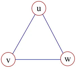
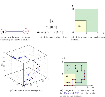
2.17 A multi-agent system consisting of three agents. . . 32

3.1 Pictorial representation of examples of sets . . . 45

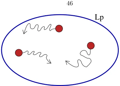
3.2 Pictorial representation of a stable level setLp . . . 46

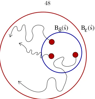
3.3 Pictorial representation of stable equilibrium state in terms ofandδballs around ˆs. 48 3.4 A graphical representation of the proof of Theorem 8. . . 49

3.5 Pictorial representation of asymptotical stability of ˆs. . . 50

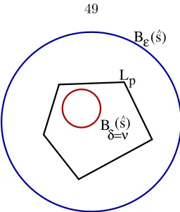
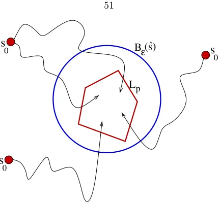
3.6 The system eventually entersLp in Theorem 9. . . 51

3.7 Lpˆ⊆Lp in Theorem 9. . . 51

3.8 Pictorial representation of aL-bounded executionπofAexog with respect to functiong. 53 3.9 Pictorial representation of a 0-bounded executionπofAexog with respect to functiong. 54 4.1 An execution of a multi-agent system consisting of three agentsA1, A2 andA3. . . 58

4.2 An example of shared-state multi-agent system and the corresponding automaton. . . 59

4.3 Generic PVS model of a shared-state multi-agent system. . . 60

4.4 Pictorial representation of the conditions of Theorem 10. . . 63

4.5 Pictorial representation of the conditions of Theorem 11. . . 63

4.6 An execution of a multi-agent system consisting of three agents where at timet, each agent can access past states of other agents.. . . 64

4.7 An execution of a multi-agent system consisting of three agents where at timet, agent A1 reads past states of agentA2 andA3. . . 65

4.8 Pictorial representation of two non-overlapping windows . . . 67

4.9 Pictorial representation of two overlapping windows. . . 68

4.10 Pictorial representation of the message-passing communication model. . . 75

4.11 An execution of a multi-agent system consisting of three agents where at timet, agent A1 receives the two messagesm2 andm3. . . 77

4.12 An execution of a multi-agent system consisting of three agents where agents execute discrete actions concurrently. . . 78

4.13 An execution of a multi-agent system consisting of three agents where agents execute actions concurrently. . . 80

(12)

5.1 Representation of a tree. The Breadth-first traversal ordering isi <BF m <BF j <BF

l <BF k.. . . 94

5.2 Examples ofq(k1,j1)for the tree in Figure 5.1.. . . 95

5.3 The communication graphG= (V, E) corresponding to matrixA whenN= 5. . . 107

5.4 A strictly diagonally dominant rooted forest of the communication graph in Figure 5.3. 108 5.5 Pictorial representation ofLk,3in the case when the system consists of 5 agents . . . 109

6.1 Architecture of the PVS Verification Framework. . . 112

6.2 Predicates and Operators defined in the PVSVectormeta-theory. . . 114

6.3 Predicates and Operators defined in the PVSMatrixmeta-theory. . . 116

6.4 System state. Refer to Figure 6.5 for the definition ofPset. . . 117

6.5 Channel Types Components of the system automaton. . . 117

6.6 Actions of the system. . . 118

6.7 Error values of agenti. . . 121

6.8 Maximum error of agentiwithin its out-going channels and within agent states. . . . 121

6.9 Assumptions on matrixA. . . 122

6.10 Assumptions on the forest of trees. . . 123

8.1 Pictorial representation of a multi-agent system whose goal is to solve a system of non-linear equations.. . . 148

(13)

List of Tables

(14)

Chapter 1

Introduction

In this Chapter, we introduce the main ideas of this Thesis. Definitions and theory are presented in later Chapters.

1.1

Thesis Contributions

This Thesis provides a theory for a new problem space and gives a mechanism to reason about it using the tools of computer science – automata and mechanical theorem proving.

Theory for a new problem domain

The Thesis introduces new theoretical tools for proving properties of multi-agent systems with con-tinuous state spaces, where states change concon-tinuously with time and where agents communicate asynchronously at discrete points over a faulty communication medium. The novel aspects of the problem domain deal with the combination of (a) continuous dynamics of agents and (b) asyn-chronous communication with discrete messages that may be delayed or lost.

(15)

An Example. A simple example of this problem space is a system withN agents,N >2, indexed

0,1, .., N−1, where agents 0 andN−1, called leaders, move in the space in some arbitrary manner,

and the goal of the remaining agents is to form a straight line with equal spacing between agents (seeFigure 2.1). Agents move according to some dynamics – for example with constant velocity or constant acceleration or some other control law. All the agents may be moving at the same time. Agents send messages containing their current positions, and these messages may be delayed or lost. When an agent receives messages, it changes its heading based on the information about other agents. If agents 0 andN−1 are stationary, a question studied in this Thesis is: “Will the system converge to the desired state?”. If agents 0 andN−1 are moving, a question is: “What is a bound (if any) between the actual state of the system and the desired state?” “How do message delay and the motion of the leaders impact the bound?”

Nondeterminism and Control. Nondeterminism is an important aspect of the problems stud-ied in this Thesis. “How should systems in which messages are lost be modeled?” For example, if one set of agents can never communicate with another set of agents because all messages between the two sets are lost, then the two sets cannot collaborate, and nothing interesting can be proven about the combined system. Models in which everyk-th message gets through are too restrictive. Models in this Thesis use an assumption of “fairness” from temporal logic that a message from one set to the other gets through “eventually”. A challenge is to integrate nondeterministic models of communication with agents that change their states continuously. For example, a mobile agent that is moving from one location to another may accelerate for the first half of the movement and deceler-ate for the second half (seeFigure 2.16(b)); or it may move at constant velocity (seeFigure 2.16(a)); or, it may choose some other control law. When this agent receives a message from another agent, the receiver cannot determine when the sender sent the message because the agents do not share a clock; the receiver may need to change direction based on the messages it receives. An agent may receive a message while it is traveling from one location to another, and the precise time and location at which the message will be received cannot be predicted. These models are very general and make weak assumptions, so that it is hard to deduce interesting properties; however, this Thesis presents theorems about convergence and stability of such systems.

(16)

the changing line. The requirement that an agent will receive a message eventually (i.e., in some arbitrary, but finite, time) is too weak because the leaders may move arbitrarily far in arbitrarily long time. Therefore, we introduce the concept of an “epoch” – a bounded time interval during which the fairness constraints are satisfied; in other words instead of merely requiring that some condition holds eventually we require that the condition holds within some time interval ∆, and we present theorems for the distance between the actual state and the goal state as a function of ∆.

Worst-Case Analysis. The Thesis analyzes worst cases rather than average cases. A worst case can be thought of in terms of a competitive game between the system and its environment. The environment knows the algorithm used by the system and the state of the system at all times. The environment takes actions to frustrate the system - for instance to maximize the distance between the actual and desired states of the system. For instance, the environment may choose to delay messages, lose messages, and reorder messages, given its knowledge of the system state. The environment must, however, satisfy the constraints imposed by the fairness assumptions.

Formalization of Systems as Automata and Mechanical Theorem Proving

Proofs of the properties can be completely axiomatic so that a theorem-proving program can check proofs mechanically. Alternatively, proofs can skip some detailed steps. In the latter case, people with knowledge of the underlying mathematical domain can check the proof, but programs may be unable to do so. Most proofs in mathematics are not provided at the level of detail that enable current theorem-proving programs to verify them. We present a theory, based on prior work on automata, which allows proofs to be verified mechanically. Automatic verification can be extremely time consuming, and we do not mechanically verify all the proofs in this Thesis. We do mechanically verify some theorems to demonstrate that the theoretical framework can be used for this purpose. A contribution of this Thesis is an automaton – theoretic representation of multi-agent systems with continuous dynamics in which agents communicate with each other through faulty communication media.

1.2

Multi-Agent Systems

In this Section, we informally describe multi-agent systems. A multi-agent system (MAS) is a collection of agents that interact with each other. Agents may cooperate towards some collective task or they may compete, each trying to achieve its individual goal. Agents may be robots, devices, software components, or, even, people.

(17)

with a subset of the system. Agents in the system may execute their actions concurrently and at different rates.

Many applications may be modeled as multi-agent systems. Homeland security [54], health monitoring [6], and habitat and environmental monitoring ([12, 60]) applications are examples of multi-agent systems. For example, in environmental applications agents may be motes, with some processing capabilities, whose goal is monitoring some quantity of the environment, such as temper-ature. Other examples of multi-agent systems can be found in robotics, where agents are team of robots; examples of these applications are agents playing some game, such as soccer [70] or “capture the flag” [23, 71]. Examples from biology are flocks of birds or shoals of fishes ([20, 10]), where agents are birds or fishes whose goal is to form and maintain a specific spatial pattern.

In this Thesis, we focus on collaborative multi-agent systems where agents interact using very simple nearest-neighbor rules. We consider hybrid systems, i.e., systems where agents may have both discrete and continuous components. For example, we consider a multi-agent system consisting of vehicles whose goal is to reach a specific desired spatial configuration. In this multi-agent system, the variables describing the state of a vehicles can be discrete or continuous. For example, a discrete variable may represent the mode of the vehicle, e.g. straight or maneuvering; this variable can drive the dynamics of the vehicles, e.g. position and acceleration, that are represented using continuous variables.

1.3

Communication Models for Multi-Agent Systems

In this Section, we present two communication models for multi-agent systems. In the first model, agents communicate via shared variables, while in the second model agents communicate by ex-changing messages over an unreliable communication medium.

In a shared-state system, agents share memory and use this memory to communicate with each other. Using this common memory, each agent exposes some variables of its own local state to other agents. Each agent is responsible for its exposed variables, as it can read and write them; an agent can only read the exposed variables of other agents. Examples of these systems are multi-threaded systems, where threads store local variables in the stack memory, while storing exposed variables in the heap memory.

(18)

The same algorithm executed over these two communication models can lead to different final system configurations. When communicating via shared variables, agents update their states using the current state of other agents. When communicating via message-passing, each agent updates its state using the latest received message. This message may contain information from an old copy of the state of some other agent, since messages may be delayed or received out-of-order. As a consequence, properties of configurations of a shared-state multi-agent system may not hold for the corresponding message-passing systems.

(a) A feasible configuration of the load balancing multi-agent system.

(b) Corresponding desired configura-tion of the load balancing multi-agent system.

Figure 1.1: Representation of a feasible and corresponding desired configuration of the load balancing multi-agent system. Nodes represent processors, edges represent dedicated communication between nodes and bars represent workload at each processor. The total amount of workload inFigure 1.1(a) andFigure 1.1(b)is the same.

1.4

Multi-Agent Systems in the Presence of Exogenous

In-puts

In this Section, we introduce the notion of exogenous inputs for multi-agent systems. These inputs are arbitrary quantities injected into the system. When injected, they can change the state of the system.

(19)

of workload; inFigure 1.1(b), we present the corresponding desired configuration where all processors store the same amount of workload. The total workloads inFigure 1.1(a)andFigure 1.1(b)are the same. We first study systems in which we are given an initial workload at each agent and no work is added or completed; the question of interest is: “Can agents interact locally so that the system state converges to the desired state?”. Exogenous inputs change the work at each agent while the load balancing algorithm is executing. New work is added and work may be completed. In this case the system may never converge to the desired state in which all agents have the same workload. The problem of interest is determining a bound (if one exists) of the error given by the distance between the actual state and the desired state.

As another example, we consider a system consisting of a network of sensors that exchange messages in an inaccessible environment. The goal of the system is to track some object traveling across some area. A system without exogenous inputs estimates the location of a stationary object. The movement of the object is modeled by exogenous inputs.

Other examples, include distributed coordination and flocking [34], vehicle formation [25,61,19] and sensor fusion [52,49] systems. In the presence of exogenous inputs, the goal state of the system can change with time. We present conditions that ensure that the system is able to track these time-varying quantities.

1.5

Motivating Example

In this Section, we present theory for proving that a general class of multi-agent systems satisfy their specifications. Agents communicate via message-passing over an unreliable communication medium. We allow for lost, delayed, duplicated, and received out-of-order messages. The goal of agents in these systems is to form and maintain a time-varying regular spatial configuration starting from some arbitrary positions.

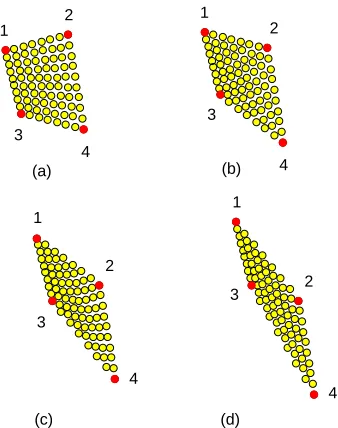
For example, in Figure 1.3 we present a sequence of snapshots of a multi-agent system whose goal is to form and maintain a regular grid. Examples of regular grids are presented inFigure 1.2 and Figure 1.5. This specific system consists of four leader agents and 76 follower agents. The desired configuration is a regular grid with corners given by the four leader agents. In this specific execution, leaders move according to the dynamics presented inFigure 1.4; inFigure 1.6, we present another sequence of snapshots of the same multi-agent systems. In this case, the dynamics of the leaders are presented inFigure 1.7.

(20)

2 1 4 3 1 2 4 3 (b) 1 (a) 1 2 3 2 4 (d) 4 (c) 3

Figure 1.2: Examples of regular grids. The cor-ner agents are depicted as dark filled circles and have identifiers ranging from 1 through 4.

(c) (d) 4 4 2 2 2 1 1 1 1 (b) (a) 4 4 2 3 3 3 3

Figure 1.3: Snapshots of the execution of a multi-agent system whose goal is to form and maintain a time-varying spatial configuration. Leader agents having have identifiers ranging from 1 through 4 and are depicted as dark filled circles. The goal configuration, depicted in Fig-ure 1.2 in the case of snapshots (a)-(d), is a regular grid with extremes given by the leader agents. The dynamics of the four leader agents is presented inFigure 1.4.

(a) (a) (a) (c) (b) (c) (b) (c) (b) (c) (d) (d) (d) (d) (a) (b) Agent 1 Agent 2 Agent 4 Agent 3

(21)

(b) (d) (c) (a) 2 1 2 1

3 4 3 ₄

1 1 2 4 3 4 2 3

Figure 1.5: Examples of regular grids. The cor-ner agents are depicted as dark filled circles and have identifiers ranging from 1 through 4.

(c) (d) 1 1 1 (b) (a) 1 2 2 2 2 3 3 3 3 4 4 4 4

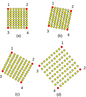
Figure 1.6: Snapshots of an execution of the multi-agent in Figure 1.3. The goal configura-tion, depicted inFigure 1.5 in the case of snap-shots (a)-(d), is a regular grid with extremes given by the leader agents. The dynamics of the leader agents are presented inFigure 1.7.

(a) (b) (c) (d) (a) (c) (d) (a) (b) (c) (d) (a) (b) (c) (d) Agent 4 Agent 3 Agent 2 Agent 1 (b)

(22)

position, because it may receive a message from a neighbor while it is traveling, and this may change its target position. An agent updates its target state using the positions stored in the received messages that are potentially old, corrupted and computed at different times.

As a specific example, we consider the case where the positions of the agents are points on the real line. The system consists of two leader agents andN−1 follower agents. The goal of the follower agents is to form an equi-spaced line with extremes given by the two leader agents. The specific equi-spaced line changes with time, since leader agents can move with arbitrary dynamics. This is the 1-dimensional version of the multi-agent system presented inFigure 1.3and Figure 1.6. In this specific system, we assume that agents have unique identifiers: the identifiers of the leader agents are 0 andN, while the identifiers of the follower agents are in the set{1, . . . , N−1}. Agents exchange messages containing agents locations. Each follower agent keeps the last message that it received from any agent with lower identifier and it also keeps the last message from any agent with higher identifier. The updating rule of the follower agent is very simple. It computes its target position as the weighted average of the values stored in these two last received messages. The weights depend on the identifiers of the senders of these two messages. It then moves towards it according to some dynamics.

Proving the correctness of systems in this class is very challenging. We must prove that the distance between the current configuration of the system and the corresponding time-varying desired configuration is bounded. In this Thesis, we present a strategy for proving correctness of these systems. We next describe the main ideas discussed in this Thesis:

1. We start by proving the correctness of a shared-state multi-agent system where agents instan-taneously update their current position with the newly computed one. In these systems, agents update their positions using the current positions of other agents. We assume that the desired final configuration does not change with time. This defines a shared-state multi-agent system with discrete, instantaneous actions. For this system, we prove that the system eventually reaches the desired configuration.

For example, in the case of the multi-agent system whose goal is forming a equi-spaced line, we have that the leader agents are stationary and, in a nondeterministic fashion, an agent chooses two other agents and updates its location with the weighted average of these other two agents. We refer to this shared-state multi-agent system as the Line-Up multi-agent system.

(23)

3. We then relax the assumption on the communication. Agents do not operate over a perfect communication medium. The medium is unreliable. We allow for messages that can be lost, delayed, duplicated or received out-of-order. Values stored in the messages in transit correspond to potentially old locations of the agents. The proof of correctness of the shared-state system remains valid in the case of message-passing systems. This is not true in general; in this Thesis, we derive conditions on the shared-state systems that ensure it. As shown in this Thesis, this class of multi-agent systems satisfies these conditions.

4. We finally model noise in the transmission and time-varying formations using exogenous inputs. This general system is able to track the time-varying final configuration. This is not true in general; in this Thesis, we derive conditions on the agents protocol in the absence of exogenous inputs and on the exogenous inputs that ensure this property.

1.6

Structure of the Thesis

In this Section, we discuss the structure of the Thesis.

Chapter 2

InChapter 2, we introduce the automaton with timed actions model. We use this model for repre-senting multi-agent systems and exogenous inputs.

An automaton with timed actions consists of a set of states, a set of initial states, a set of timed actions, an enabling predicate and a transition function. In the case of the multi-agent system, the state space of the automaton models the state of its agents and, in case of message-passing communication, the state of the communication medium. The set of actions along with the enabling condition and transition function models the behaviour of the agents of the system. In the case of exogenous inputs, the state space of the automaton models the state space of the multi-agent system and its set of actions models the behaviour of these exogenous injections. We assume that exogenous inputs can modify any agent in the system.

(24)

Chapter 3

In Chapter 3 we discuss properties of automata with timed actions. We use these properties for proving correctness of the corresponding multi-agent systems.

In this Chapter, we introduce the notion of equilibrium state. An equilibrium state is a fixed point of the executions of the automaton. Equilibrium states model goal configurations of multi-agent systems. For example, the goal configuration of the Line-Up multi-agent system is an equilibrium state of the corresponding Line-Up automaton.

In this Chapter, we introduce stability and convergence properties. Informally, an equilibrium state is stable if every execution of the automaton that starts close to the equilibrium state remains close to it. The system converges to an equilibrium state if any fair execution of the automaton that starts close to the equilibrium state converges to it. In this Chapter, we provide sufficient conditions on the automaton that ensure stability and convergence. We also discuss properties of automata in the presence of exogenous inputs. When injecting exogenous inputs, we are interested in the robustness of the system. We model this robustness property with the notion of bounded automaton. An automaton in the presence of exogenous inputs is bounded if eventually-always the distance between the system and the set of equilibrium states of the automaton in the absence of exogenous inputs is bounded.

The material covered in this Chapter has been published in [14]. Our work extends the work of [66] to systems with timed actions, in the special case of metric state space.

Chapter 4

InChapter 4 we discuss stability and convergence properties of multi-agent systems. We consider both shared-state and message-passing multi-agent systems.

We first discuss properties of shared-state multi-agent systems. We model these systems as automata with discrete or timed actions. We prove correctness of these systems using the results ofChapter 3.

(25)

We finally discuss multi-agent systems with concurrent actions. In these systems, agents can execute actions concurrently. For example, in the Line-Up multi-agent system with concurrent actions, multiple agents can move at the same time. We model both shared-state and message-passing systems with concurrent actions and derive conditions that ensure stability and convergence of these systems.

The material of this Chapter has been partially presented in [16] and extends the work of [66,8] where they prove stability and correctness of multi-agent systems with concurrent discrete actions.

Chapter 5

InChapter 5we discuss the correctness of a general class of iterative schemes. The goal of systems in this class is solving a system of linear equations of the formA·x=b. These systems iteratively compute vector xstarting from an initial guess vectorx0. These are decentralized schemes where each agent is responsible for solving a specific variable using a specific equation of the system of linear equations. For example, agenti would be responsible for computing x(i) using as updating rule thei-th equation of the system. We consider both shared-state and message-passing multi-agent systems.

We, first, consider shared-state multi-agent systems. We prove the correctness of schemes in this class using the results in Chapter 3. We require the matrix Ato satisfy specific assumptions. We, then, consider message-passing multi-agent systems. In these systems, agentirepeatedly broadcasts a message containing the current value ofx(i). Agenti uses thei-th equation as its updating rule. In this equation, variablex(i) is the only unknown, since agentiuses the last message received from agentj to representx(j) for allj6=i. We prove correctness of message-passing systems using results ofChapter 4.

In this Chapter, we discuss a linear robot pattern formation protocol that can be modeled as a multi-agent system whose goal is solving a system of equations. This protocol is a special case of the Line-Up multi-agent system. We derive its proof of correctness from the convergence property of systems in this class.

The material covered in this Chapter has been published in [14]. It extend the work of [28] in the linear case, and the work of [18] relaxing some assumptions on the equations in the system.

Chapter 6

(26)

systems [36,46,45,35,38].

In this Chapter, we detail the structure of the framework. It consists of three main libraries. The first library describes the state space, initial states, actions, enabling condition and transition function of the message-passing multi-agent system. The state of the system consists of the state of the agents and the state of the communication medium. The second library encodes the proof of correctness of these systems in PVS. The third library presents auxiliary lemmas on predefined data structures such as vectors and matrices.

When using this framework, the end-user is required to discharge some assumptions on the matrix

A. As an example, we apply our verification framework for proving correctness of the robot pattern formation protocol described inChapter 5.

The material covered in this Chapter has been published in [56, 57]. Our work follows a very large body of literature where theorem provers have been used for modeling [29, 30, 11, 37] and verification [33, 27,44]. A theorem prover is an appropriate tool when modeling nondeterministic systems with dense state spaces. Other tools that rely on exhaustive state space exploration, such as model checkers, may present difficulties when dealing with this issue. However, there are some exceptions. For example, in [31], the author checks the time to reach agreement of a consensus protocol using the UPPAAL model checker [7]. The author is able to reduce the state space of the system using a key compositional property of the protocol.

Chapter 7

InChapter 7we discuss properties of the multi-agent systems in the presence of exogenous inputs. We prove that the system in the presence of exogenous inputs is bounded, if the multi-agent system in the absence of exogenous inputs and the exogenous inputs injected in the system satisfy specific properties. These conditions require the system in the absence of exogenous inputs to execute additive protocols and require the exogenous inputs to be uniformly bounded quantities added to the agents.

(27)

(28)

Chapter 2

Formal Models for Multi-Agent

Systems

In this Chapter, we present formal models for multi-agent systems. We use these models to formally represent multi-agent systems and describe their behaviors.

InSection 2.1we review the automaton model. InSection 2.2we present a new extension of the automaton model, that allows modeling systems with continuous-time actions. In Section 2.3 we introduce a novel notion of fairness for automata. This notion of fairness will be used throughout the Thesis. InSection 2.4we discuss an automaton that models multi-agent systems in the presence of exogenous inputs. Finally, inSection 2.5we relate the main results of this Chapter to the literature.

2.1

Automata

In this Section, we review the automaton model and present an example.

2.1.1

Automaton Model

We refer to [5] for a discussion of the concept of automata. Formally, anautomaton has the following structure.

Definition 1. An automaton is a quintuple (S, S0, A, E, T)consisting of

• nonempty set of states S

• nonempty set of start (initial) statesS0

• a set of actions A

• an enabling predicate E:S×A→ B,

(29)

The set B denotes the set of boolean values,B ={true, f alse}. Fors ∈S anda ∈A, E(s, a) holds if and only if action a can be executed in the states. If this is the case, we say that a is

enabled ins. For convenience, we writes−→a s0 to denote (s, a, s0)∈T.

The semantic of an automaton is defined in terms of its executions; these describe the behavior of the system.

Definition 2. An execution fragment is a possibly infinite alternating sequence of states and actions s0, a0, s1, a1, . . .such that si+1=T(si, ai)andE(si, ai)holds.

An execution fragment is a system execution if s0∈S0.

Given an executionπ of the system, we denote byπ.f statethe first state of the execution. Ifπ

is finite, we denote byπ.lstatethe last state of the execution.

We next introduce the concept of reachability. Given s, s0 ∈S, we say that s0 isreachable from s, if there exists a finite (possibly empty) execution fragment starting from sthat reaches s0. We denote byRF(s) the set of states reachable froms, defined formally as:

Definition 3. Given s∈S, the setRF(s)is defined as

RF(s) ={s0∈S | ∃π:π.f state=s∧π.lstate=s0}

We can extend this definition to a set of states ˆS. The set of reachable states from ˆS is the union of the set of reachable states from its elements. Formally,

Definition 4. Given Sˆ∈S,

RF( ˆS) ={s0∈S| ∃ˆs∈S,ˆ ∃π:π.f state= ˆs∧π.lstate=s0}

We introduce the reachable predicate as follows:

Definition 5. Given s∈S,

r(s)≡(s∈RF(S0))

The predicate holds ifsis reachable from some initial state. Ifr(s) holds, we say thatsisreachable. Automata are used for formalizing discrete-time systems. Actions of the automaton have constant discrete execution times. When an action is executed by the automaton, the clock of the system is advanced by some fixed discrete time. For this reason, these automata are usually called discrete automata.

2.1.2

Line-Up Automaton

(30)

(stored in the vector x0), and, through interactions, their goal is to converge to a configuration where agents are located, in order, at equidistant points on a straight line with extremesx0(0) and

x0(N). Without loss of generality, we present the one-dimensional version of the protocol, where agent positions are real values. Figure 2.1 shows two configurations of the Line-Up multi-agent system when the system consists of ten agents; Figure 2.1(a) represents a generic configuration while Figure 2.1(b) represents the desired final configuration, where all agents are in order and equispaced on the line.

0 1 2 3 4 5 6 7 8 9

(a) Pictorial representation of an initial state of the Line-Up multi-agent system.

0 1 2 3 4 5 6 7 8 9

(b) Pictorial representation of the corresponding goal state.

Figure 2.1: A Line-Up multi-agent system consisting of 10 agents.

Agents update their state in a nondeterministic fashion. Agent i chooses nondeterministically two agentsl, r withl < i < r and sets its new position x0 as the weighted average of the positions ofl, r:

x0= r−i

r−lx(l) + i−l

r−lx(r) (2.1)

where x is the vector of agent positions. We denote this updating rule by avgl,i,r. Figure 2.2

pictorially represents this updating rule for a given example; Figure 2.2(a) represents agents l, i, r

beforeiexecutes the updating rule andFigure 2.2(b)represents the same agents after the execution of the rule. As discussed before, only agent i modifies its position; its new position is a linear combination of the positions ofl, r. Notice that, in the case whenl=i−1 andr=i+ 1, we have thatx0 is the average of the positions ofx(i−1) andx(i+ 1), since r_r−₋i_l = _ri−₋l_l =1₂.

The goal configuration of the Line-Up system is the vector ˆxwhere∀i≤N

ˆ

x(i) =N−i

N x0(0) + i

Nx0(N) (2.2)

l

i r

(a) Configuration of agentsl, iandr.

l i r

(b) Configuration of agentsl, iandr after agenti exe-cutes the updating rule.

(31)

We refer toFigure 2.1(b)for a pictorial representation of the desired goal configuration for a system of 10 agents.

The automaton modeling the Line-Up multi-agent system has the following structure:

• S =_RN+1_{, since the state space of each agent is}

R.

• S0 ={s0}, withs0 =x0,

• A={Ai}i∈I withAi={avgl,i,r}l<i<r,

• E:S×A→true

• T :S×A→S, defined as∀a=avgl,i,r∈A,∀s∈S,

T(s, a) =

s(0), s(1), s(2), . . . ,r−i r−ls(l) +

i−l

r−ls(r), . . . , s(N)

For this model, agents 0 andN are stationary.

As presented inEquation 2.1, the goal configuration of the Line-Up system is the state ˆswhere ∀i≤N

ˆ

s(i) = N−i

N s0(0) + i

Ns0(N) (2.3)

withs0∈S0.

InFigure 2.3, we present a formalization of the system in the PVS theorem prover. The system consists ofN+ 1 agents, withN >0. Each agent has a unique identifier. This is a natural number in the interval [0, N]. In PVS, the type of agent identifiers is I. The state space of each agent is the set of real numbers. The state space of the system is defined by the function S, that maps each agent identifier to a real value. This theory has an input parameter given by the state s0. This parameter stores the initial configuration of the system. The set of initial states is encoded in PVS using the initial state predicate start?. The set of actionsA of the system consists of the actionavg. This action has three parameters; these are identifiers of three agents: i,left,right. As encoded in the enabling condition predicate E, this action can be executed only if agent i is properly contained in the interval [left, right]. When executing this action, the post-state of the action is equal to the pre-state, with the exception of thei-th coordinate. This entry stores the weighted average ofs(left)ands(right). The execution of this action is encoded in PVS by the transition functionT.

2.2

Automata with Timed Actions

(32)

% N u m b e r of a g e n t s of the s y s t e m . N : p o s n a t

% A g e n t I d e n t i f i e r .

% It is a n a t u r a l n u m b e r in the i n t e r v a l [0 , N ]. I : T Y P E = u p t o ( N )

% S t a t e d e f i n i t i o n .

% A s t a t e m a p s e a c h a g e n t i d e n t i f i e r i n t o a r e a l v a l u e . S : T Y P E = [ I - > r e a l ]

% PVS meta - t h e o r y .

% s0 is an i n p u t of the t h e o r y .

% s0 r e p r e s e n t s the i n i t i a l c o n f i g u r a t i o n of the s y s t e m . L i n e U P [ s0 : S ]: T H E O R Y

B E G I N

i , left , r i g h t : VAR I

% A c t i o n set of the s y s t e m . A : D A T A T Y P E

B E G I N

% avg a c t i o n

% its p a r a m e t e r s are left , i , r i g h t avg ( left , i , r i g h t ): avg ?

END A

s : VAR S a : VAR A

% I n i t i a l S t a t e P r e d i c a t e . s t a r t ?( s ): b o o l = ( s = s0 )

% E n a b l i n g P r e d i c a t e . E ( s , a ): b o o l =

C A S E S a OF

% avg is e n a b l e d if left < i < r i g h t

avg ( left , i , r i g h t ): ( left < i ) AND ( i < r i g h t ) E N D C A S E S

% T r a n s i t i o n F u n c t i o n . T ( s , a ): S =

C A S E S a OF

% A g e n t i s e t s its v a l u e to the w e i g h t e d a v e r a g e of % the v a l u e s of l ef t and r i g h t

avg ( left , i , r i g h t ): LET

w _ l e f t : p o s r e a l = ( right - i )/( right - l e f t ) , w _ r i g h t : p o s r e a l = ( i - l e f t )/( right - l e f t ) IN

s W I T H [( i ):= w _ l e f t * s ( l e f t ) + w _ r i g h t * s ( r i g h t )] E N D C A S E S

END L i n e U P

(33)

used for modeling systems with continuous-time dynamics, such as mobile multi-robot systems. We first present the model and discuss it. We then define the concepts of executions and reach-ability for this automaton. We then extend the meaning of the temporal operators always 2 and eventually 3 to this class. We finally present an example and relate this model to other timed system models.

2.2.1

Automaton Model

Informally, an automaton with timed actions is a generalization of the discrete automaton model presented in Section 2.1. An automaton with timed actions has a state space S, a set of initial statesS0 and a set of actions A. Unlike the discrete automaton model, actions have time duration. Formally,

Definition 6. A automaton with time actionsAis a tuple (S, S0, A, E, T)consisting of

• nonempty set of states S,

• nonempty set of start (initial) statesS0,

• a set of actions A,

• an enabling predicate E:S×A→ B,

• a transition functionT :S×A→(_T→S)with

T={[0, τ] |≤τ <∞}

such that ∀s∈S, a∈A,

T(s, a)(0) =s

The duration and behaviour of the actions ofAare encoded in the transition functionT. Parameters ofT are a state inSand an action inA. By construction of the transition function, we have that the same action can have different time duration and behaviour when executed at different states. The transition functionT specifies the behaviour of the action throughout its duration. Given a states

and an actiona,T(s, a) defines a mapping from a closed finite time interval to the state space ofA. The state T(s, a)(0) is equal to states, sinceT(s, a)(0) specifies the behavior of the action at the beginning of the interval. The closed finite interval is lower bounded by some constant >0, i.e. we do not allow for Zeno executions. As an example,Figure 2.4presents a pictorial representation of the behaviour of a timed actiona. The system consists of a single real-valued variable. Whena

(34)

1

0

t

T(s=0,a)(t)

state

time

Figure 2.4: Pictorial representation of behavior of a timed action. The system consists of variable

x, that evolves with constant velocity from value 0 to value 1 for 1 time unit.

with constant velocityv= 1. Mathematically, the behaviour of the timed actionacan be expressed using the functionT as follows: ∀t∈[0,1],T(s, a)(t) =s+v·t, withs= 0 andv= 1.

In our model, the set of actions has a special action, called no-op action. This action advances the time of the automaton, in the case when the execution of the system reaches a state where no action is enabled. We require this action since the execution cannot move forward in time if no action is enabled. This is analogous to the skip action in UNITY [15]. This action is enabled in states∈S if no other action is enabled ins, i.e.

E(s,no-op) = (∀a∈A, a6= no-op, ¬(E(s, a)))

The time duration of this action insis

T(s,no-op) = [0, ]→S

When executed ins, it does not modifys, i.e. ∀t∈[0, ] we have that

T(s,no-op)(t) =s

This action advances the execution of the automaton bytime units.

This model generalizes the discrete automaton model presented in Section 2.1. An automaton Acan be encoded as an automaton with timed actionsAtime. AutomatonAtimehas the same state

space, initial states and actions ofA. Actions ofAcan be modeled as actions in Atime as follows.

(35)

• Stime=S

• S0time=S0

• Atime=A

• ∀s∈Stime, a∈Atime,Etime(s, a) =E(s, a)

• ∀s∈Stime, a∈Atime,T(s, a) : [0,1]→S with

∀t <1 : Ttime(s, a)(t) =s Ttime(s, a)(1) =T(s, a)

2.2.2

Executions and Reachability

In this Section, we extend the concepts of executions and reachability to automata with timed actions. Throughout the Thesis, given an automaton with timed actionsA= (S, S0, A, E, T), given

s∈S, a∈A, we denote byfs,athe functionT(s, a), and byτs,a the right extreme of the domain of fs,a, i.e. fs,a: [0, τs,a]→S; by construction,τs,ais finite. We denote by ends,a the statefs,a(τs,a),

i.e. it is the state resulting into the evaluation of the function fs,a at the right extreme of the

interval. For convenience, we denote (s, a, fs,a)∈T as s a

−→ends,a.

s₀

a

0

s

0, τ

s

1,a1 τ a

0

s

0, τ +

a₀ a₁

s₁ _s

0 a0

= end _,

s₂ _s

1 a1

= end _,

0 _time

state

Figure 2.5: Pictorial representation of an end-state execution fragment. Dark filled circles represent end-states of the execution and arrows represent the execution of the actions. This end-state ex-ecution fragment starts at state s0 and executes actions a0, a1, . . .. When executed from states0, action a0 has time duration τs0,a0. Action a1 has time duration τs1,a1 when executed from state

s1= ends0,a0.

(36)

Definition 7. An end-state execution fragmentπis a possibly infinite alternating sequence of states and actions π=s0, a0, s1, a1. . .such that si+1=endsi,ai, andE(si, ai)holds.

If the execution is finite, i.e. π=s0, a0, s1, a1. . . aN−1, sN, then its time duration isτ=PN_i₌₀−1τsi,ai.

An end-state execution fragment starts from a states0 and executes actiona0 from state s0. The execution ofa0 has a time durationτs0,a0 and end-state equal tos1. In states1, it executes action

a1that has time durationτs1,a1 and end-state equal tos2and so on. If 0 is the time of the execution

πat state s0, we have that the time of πat state s1 isτs0,a0, the time of the execution at states2 is τs0,a0+τs1,a1 and so on. Given πwe denote by t0, t1, . . . the possibly infinite sequence of times withtibeing the time ofπat statesi. This sequence of times can be defined recursively: t0= 0 and

ti =ti−1+τsi,ai. Figure 2.5presents an example of end-state execution fragment; this fragment starts ats0 and executes actionsa0, a1, . . ..

s₀

s₁,a₁

f

a₀ s₀,

f

s₁

a₀ s₀, τ

s₁,a₁ τ a₀ s₀, τ + s₂ 0 a 1 a 2 a 0 _time state

action action action

Figure 2.6: Pictorial representation of the function describing the end-state execution fragment depicted in Figure 2.5. In this specific example, ˆt = 0. Dark filled circles represent end-states of the execution. The curve in the time interval [0, τs0,a0] represents the behavior of action a0 when executed in states0. This behaviour is described by functionfs0,a0. The curve in the time interval [τs0,a0, τs0,a0+τs1,a1] represents the behavior of actiona1when executed in states1. This behavior is described by functionfs1,a1.

In general, given an end-state infinite execution fragment π=s0, a0, s1, a1. . ., and a time ˆt we have thatπcan be represented as a function ˆπ: [ˆt,∞)→S such that∀i∈_N:

(ˆπ(ti) =si)∧(E(ˆπ(ti), ai))∧(∀t∈[ti, ti+1] : ˆπ(t) =fsi,ai(t))

where the infinite sequence of times t0, t1, . . .is recursively defined as t0 = ˆt andti =ti−1+τsi,ai. We next briefly discuss these three conditions: (1) the first condition ensures that si is the state

of the execution at time ti, (2) the second condition ensures that action ai is enabled in state si,

(3) the third condition ensures that action ai is executed in state si and, together with the first

condition, that the post-state of the execution is si+1. For example, Figure 2.6 represents the function corresponding to the end-state execution fragment inFigure 2.5.

(37)

that the function corresponding toπis defined as ˆπ: [ˆt,ˆt+τ]→S, withτ being the time duration of π. In this specific case, we have that the sequence of times is finite, and given byt0, t1, . . . , tN

witht0= ˆtandti=ti−1+τsi,ai. The conditions on the function are the same as the conditions for the case of the infinite execution fragment, and, thus, they are not reported.

We denote byEend−statethe set of all functions corresponding to end-state execution fragments

of the system. Throughout this Thesis, we do not distinguish between execution fragments and their functional representations. We use them interchangeably.

In our model, actions have time duration. For this reason, feasible execution fragments may start during the execution of some action of the fragment. Also, in case of finite fragments, they may end during the execution of some action or they may start and end during the execution of some action. We refer toFigure 2.7,Figure 2.8andFigure 2.9for a pictorial representation of these three cases. The finite fragment in Figure 2.8starts at state s0 and executing actiona0 in states0 reaches states1. It then initiates actiona1starting froms1for onlyt−τs0,a0 time units. It stops before the action is completed at timeτs0,a0+τs1,a1. In our model, this fragment is a valid execution fragment. The fragment inFigure 2.9starts from a states0₀withs0₀=T(s0, a0)(t) andt >0. The fragment starts while actiona0 is executing. Then, it reaches s1 and executesa1, and so on. In our model, also this fragment is a valid execution fragment.

We next introduce the sub-fragment operator.

Definition 8. Given an end-state execution fragment π: ∆→ S and a time interval ∆ˆ, the sub-fragment ofπwith respect to ∆ˆ, denoted bysub(π,∆)ˆ , is a functionπˆ : ˆ∆→S such that

• ∆ˆ is a sub-interval of ∆ and

• πˆ is the restriction ofπ to∆ˆ.

Figure 2.7,Figure 2.8and Figure 2.9are examples of sub-fragments of the end-state execution fragment presented in Figure 2.6. In the sub-fragment depicted in Figure 2.7 the time interval

ˆ

∆ is [t1, t2]; in the sub-fragment depicted in Figure 2.8, ˆ∆ = [0, t]; in the sub-fragment depicted inFigure 2.9, ˆ∆ = [t,∞).

If ˆ∆ is a prefix of ∆, we say that ˆπ is a prefix of π. For example, the execution fragment inFigure 2.8 is a prefix of the end-state execution fragment presented inFigure 2.6since ˆ∆ = [0, t] is a prefix of [0,∞). Instead, if ˆ∆ is a suffix of ∆, we say that ˆπ is a suffix ofπ. For example, the execution fragment inFigure 2.9is a suffix of the end-state execution fragment presented inFigure 2.6 since ˆ∆ = [t,∞) is a suffix of [0,∞).

Given this operator, we next define the notion of execution fragment.

(38)

s₀

a₀ s₀, f s₁ s₂ a 0 s 0, τ _s

1,a1 τ

+ s

1,a1 f a 0 s 0, τ 1

t t2

s₀’

’ s₂

∆^

0 _time

state

Figure 2.7: Pictorial representation of a finite sub-fragment of the end-state execution fragment depicted in Figure 2.6. This sub-fragment has domain ˆ∆ = [t1, t2]. It starts in state s00 with

s00 = T(s0, as)(t1) and it ends in state s02 with s20 = T(s1, a1)(t2−τs0,a0). It executes action a0 starting from time t1, then it executes action a2 for t2−τs0,a0 time units. The dark solid line represents the behavior of the actions in this sub-fragment, while the dashed lines represent the behavior of the actions in the end-state execution fragment presented inFigure 2.6.

Given an execution fragment π, we denote byπ.f statethe first state ofπand π.lstatethe last state ofπ, if the executionπ is finite. Ifπ is a finite execution fragment, then the time interval ˆ∆ is closed and finite. Instead, if πis an infinite end-state execution fragment, then ˆ∆ can be either closed and finite or left-closed and infinite. The function inFigure 2.8is an execution fragment since it is the restriction of the end-state execution fragment presented inFigure 2.6to the interval [0, t]. Similarly, the function inFigure 2.9is an execution fragment since it is restriction of the end-state execution fragment presented inFigure 2.6 to the interval [t,∞).

Given an end-state execution fragment π we denote by Suffix(π) the set of suffix execution fragments of π. If π is an infinite execution fragment, we have that the set Suffix(π) is infinite. Instead, ifπis a finite execution fragment, we have that the set Suffix(π) contains a finite number of execution fragments.

We denote byEthe set of execution fragments and byE∞the set of infinite execution fragments (i.e. E∞⊂ E). By construction,E is the closure ofEend−stateunder the sub-fragment operator. An

execution fragmentπ: ∆→S is an execution, if 0 is the left extreme of ∆ andπ.f state∈S0. We denote byES0the set of executions and byES0,∞ the set of infinite executions.

Given a state s∈S, we next define the set of reachable states froms.

Definition 10. Givens∈S, the set of reachable states fromsis

RF(s) ={s0 | ∃π∈ E : π.f state=s∧π.lstate=s0}

(39)

s₀

a₀ s₀, f

s₁

s₂

a

0

s

0,

τ _s

1,a1 τ

+ s

1,a1 f

a

0

s

0, τ

s₂’

∆^

0 _t _time

state

Figure 2.8: Pictorial representation of a prefix of the end-state execution fragment depicted in Fig-ure 2.6. This prefix has domain ˆ∆ = [0, t]. It starts in state s0 and it ends in state s02 with

s02=T(s1, a1)(t−τs0,a0). It executes actiona0starting from states0, it then executes actiona2for

t−τs0,a0 time units. The dark solid line represents the behavior of the actions in this sub-fragment, while the dashed line represents the behavior of the actions in the end-state execution fragment presented inFigure 2.6.

Definition 11. GivenSˆ∈S, the set of reachable states from the setSˆis

RF( ˆS) ={s0 | ∃ˆs∈S,ˆ ∃π∈ E : π.f state= ˆs∧π.lstate=s0}

2.2.3

Temporal Operators

In this Section, we extend the definitions of the temporal operators always (2) and eventually (3). Before proceeding with these definitions, we review the concept of predicate. A predicateP on the state space of the automaton A is a function that returns a boolean value, i.e. P : S → B. We say that predicate P holds in state s ∈S, if P(s) = true. We next extend this definition to execution fragments and automata. PredicateP holds for an execution fragmentπ, denoted byPπ,

ifP holds at π.f state, i.e. if predicateP holds at the initial state ofπ. A predicateP holds for an automatonAifP holds for all system executions.

The2operator is defined as follows.

Definition 12. Given a predicateP,

• 2P holds for an execution fragmentπ, denoted by2πP, if ∀ˆπ∈Suffix(π) : Pπˆ

• 2P holds for an automatonA= (S, S0, A, E, T), if ∀π∈ ES0,∞ : 2πP

(40)

s

1,a1 f a 0 s 0, f s₀ s₁ s₂

s₁,a₁

τ

a₀ s₀,

τ +

a₀ s₀,

τ s₀_’

∆^

0 _t _time

state

Figure 2.9: Pictorial representation of a suffix of the end-state execution fragment depicted in Fig-ure 2.6. This suffix has interval ˆ∆ = [t,∞). This is an infinite sub-fragment that starts in state

s0₀ with s0₀ = T(s0, a0)(t). It executes action a0 starting from time t, then it executes action a2 and so on. The dark solid line represents the behavior of the actions in this sub-fragment, while the dashed line represents the behavior of the actions in the end-state execution fragment presented inFigure 2.6.

s₀

s

1,a1

f a 0 s 0, f s₁ s₂ a₀ s₀,

τ

s

1,a1 τ

a₀ s₀,

τ + s₀ < s₁ < 0

P

time state

Figure 2.10: Execution fragment where2P holds; predicateP holds insifs∈[ˆs0,sˆ1]. The shaded area represents the region where predicateP holds.

Similarly, the eventually operator is defined as follows.

Definition 13. Given a predicateP,

• 3P holds for an execution fragment π, denoted by3πP, if∃ˆπ∈Suffix(π) : Pˆπ

• 3P holds for an automatonA= (S, S0, A, E, T), if∀π∈ ES0,∞ : 3πP

3 P holds for a possibly infinite execution fragment π if the predicate P holds for some suffix execution fragments ofπ. Therefore,3P holds forπifP holds in some state ofπ. InFigure 2.11, we presents an execution fragment satisfying 3 P and in Figure 2.12, we represent an execution fragment where 3 P does not hold. 3 P holds for an automaton A if it holds for all its infinite executions.

(41)

s₀

s

1,a1

f

a₀ s₀,

f

s₁

s₂

a₀ s₀,

τ

s₁,a₁

τ

a₀ s₀,

τ +

s₀

<s1

<

0

P

time state

Figure 2.11: Execution fragment where3P hold; predicate P holds insifs∈[ˆs0,ˆs1]. The shaded area represents the region where predicateP holds.

s₀

s

1,a1

f

a₀ s₀,

f s₁ s₂ a 0 s 0, τ s

1,a1 τ a 0 s 0, τ + s₀

<s1

<

P

0 _time

state

Figure 2.12: Execution fragment where 3 P does not hold; predicate P holds ins if s ∈[ˆs0,sˆ1]. The shaded area represents the region where predicateP holds.

Lemma 1.

2P ≡(RF(S0)⊆P)

Proof. It follows directly from the definition of2P and reachability.

We next discuss the meaning of the main temporal logic formulas used in this Thesis. These are 32P,2(P ⇒3Q) and2(P ⇒2P).

We start discussing 32P. Informally, 32P holds for an execution if there exists a time t in the execution such that the predicate P holds after timet. Formally, given an executionπ, 32P

(42)

s₀

a₀ s₀,

f

s₁

a₀ s₀,

τ

s₁,a₁

τ

a₀ s₀,

τ + s

1,a1

f

s₂ s₁

<

s₀

<

0

P

time state

Figure 2.13: Execution fragment where 32 P holds; predicate P holds in s if s ∈ [ˆs0,sˆ1]. The shaded area represents the region where predicateP holds.

all its executions. We next formally derive the meaning of this formula:

32P ≡ (∀π∈ ES0,∞ : 3π(2P))

≡ (∀π∈ ES0,∞ : ∃ˆπ∈Suffix(π) : 2πP)

≡ (∀π∈ ES0,∞ : ∃ˆπ∈Suffix(π) : ∀¯π∈Suffix(ˆπ) :P(¯π.f state)) ≡ (∀π:_R≥0→S, π(0)∈S0 : ∃t0≥0 : ∀t≥t0 :P(π(t)))

We next discuss the meaning of the temporal logic formula2(P ⇒3Q). Informally, the formula 2(P ⇒3Q) holds for an execution fragment, if for all states in the execution satisfying P there exists a state later in the execution satisfyingQ. Formally, given an executionπ,2(P ⇒3Q) holds forπ if for all t≥0, such thatP(π(t)), there exists t0 ≥t, such that Q(π(t0)). InFigure 2.14, we present an execution where2(P ⇒3Q) holds. Similarly, the temporal logic formula2(P ⇒3Q) holds for an automatonAif it holds for all its executions. We next formally derive the meaning of this formula:

2(P ⇒3Q) ≡ (∀π∈ ES0,∞ : 2π (P ⇒3Q))

≡ (∀π∈ ES0,∞ : ∀ˆπ∈Suffix(π) : (P ⇒3Q)ˆπ)

≡ (∀π∈ ES0,∞ : ∀ˆπ∈Suffix(π) : (Pˆπ⇒3πˆQ))

≡ (∀π∈ ES0,∞ : ∀ˆπ∈Suffix(π) : (P(ˆπ.f state)⇒ ∃π¯∈Suffix(ˆπ) : Q(¯π.f state))) ≡ (∀π:_R≥0→S, π(0)∈S0 : ∀t≥0 : (P(π(t))⇒ ∃t0≥t : Q(π(t0))))

We finally discuss the meaning of temporal formula 2(P⇒2P). Informally, the formula 2(P ⇒2P) holds for an execution fragment, if for all states in the execution fragment ifP holds in the state then P continues to hold forever. Formally, given an executionπ,2(P ⇒2P) holds

(43)

s₀ a 0 s 0, f s₁ a 0 s 0, τ s 1,a1 τ a 0 s 0, τ + s

1,a1 f s₂ < s₁ s₀ < < s₂ < s₃ 0

Q

P

time state

Figure 2.14: Execution fragment where 2(P ⇒3Q) holds; predicate P holds in s if s ∈ [ˆs0,sˆ1] and predicateQholds insifs∈[ˆs2,sˆ3]. The shaded areas represent the regions where predicateP and predicateQhold.

present two execution where2(P ⇒2P) holds. Similarly, the temporal logic formula2(P ⇒2P) holds for an automatonAif it holds for all its executions. We next formally derive the meaning of this formula:

2(P ⇒2P) ≡ (∀π∈ ES0,∞ : 2π (P⇒2P))

≡ (∀π∈ ES0,∞ : ∀ˆπ∈Suffix(π) : (P ⇒2P)ˆπ)

≡ (∀π∈ ES0,∞ : ∀ˆπ∈Suffix(π) : (Pπˆ⇒2πˆ P))

≡ (∀π∈ ES0,∞ : ∀ˆπ∈Suffix(π) : (P(ˆπ.f state)⇒ ∀¯π∈Suffix(ˆπ) : P(¯π.f state))) ≡ (∀π:_R≥0→S, π(0)∈S0 : ∀t≥0 : (P(π(t))⇒ ∀t0 ≥t : P(π(t0))))

2.2.4

Line-Up automaton with dynamics

In this Section, we present the Line-Up multi-agent system with dynamics and model it using the automaton with timed actions framework. This agent system generalizes the Line-Up multi-agent system presented in Section 2.1.2. The system consists of N + 1 agents whose goal is to converge to a configuration where agents are located, in order, at equidistant points on a straight line with extremes given by the initial positions of agent 0 and agentN.

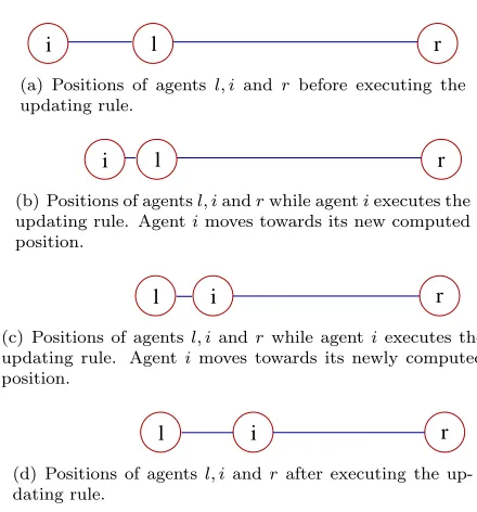
In the Line-Up multi-agent system with dynamics, the updating rule of agenti, presented in Fig-ure 2.15, is defined as follows. Agent i chooses two other agents l, r with l < i < r, it computes its new position x0 using the formula defined in Equation 2.1, and continuously moves from its current location to its destination position x0. We suppose that agent i reaches x0 in finite time. For example, agent i can move towards x0 with constant velocity or it can instantaneously jump from its current position to its newly computed one. The jump dynamics models the protocol of the Line-Up multi-agent system presented inSection 2.1.2.

(44)

l

i r

(a) Positions of agents l, iand rbefore executing the updating rule.

l

i r

(b) Positions of agentsl, iandrwhile agentiexecutes the updating rule. Agentimoves towards its new computed position.

l i r

(c) Positions of agentsl, iand rwhile agentiexecutes the updating rule. Agentimoves towards its newly computed position.

l i r

(d) Positions of agentsl, iandr after executing the up-dating rule.

Figure 2.15: Agent i executes the updating rule and moves from its current position to the newly computed one.

the following structure:

• S =_RN+1_{, since the state space of each agent is}

R.

• S0 ={s0}, withs0 =x0,

• A={Ai}i∈I withAi={avgdl,i,r}l<i<r,

• E:S×A→true

• T :S×A→(_T→S), defined as∀s∈S,∀a≡avg_dl,i,r∈A,

∀j6=i,∀t≤τs,a : (T(s, a)(t))(j) =s(j)

∀t≤τs,a : (T(s, a)(t))(i) =fs,a(t)

withfs,a: [0, τs,a]→S having

fs,a(0) = s(i) fs,a(τs,a) =

r−i r−ls(l) +

i−l r−ls(r)

In this automaton, agents 0 andN are stationary. The remaining agents move toward their destina-tion posidestina-tions computed using the formula inEquation 2.1. The functionfs,amodels the dynamics

(45)

this means that agent i can have different dynamics when starting from different states. In gen-eral, in our model, different agents can have different dynamics and the duration of their actions can be different as well. Examples of feasible dynamics for agent iare presented in Figure 2.16(a) andFigure 2.16(b).

The goal state of the automaton is the same goal state of the automaton presented inSection 2.1.2. We refer toEquation 2.3for its definition.

f_{s ,a}

τ_{s ,a} R

time 0

(a) Agenti moves with constant velocity forτs,atime units.

τ_{s ,a}

f_s_,a

0 R

time

(b) Agent imoves with constant acceleration for τs,a

2 time units, then it moves with constant de-celeration for τs,a

2 time units.