Properties of time averages in a risk management simulation

(1)

Munich Personal RePEc Archive

Properties of time averages in a risk

management simulation

Bell, Peter Newton

7 May 2014

Online at

https://mpra.ub.uni-muenchen.de/55803/

(2)

Properties of time averages in a risk management simulation

Peter N. Bell

Department of Economics, University of Victoria

This research was supported by the Joseph-Armand Bombardier Canada Graduate Scholarship –

Doctoral through the Social Sciences and Humanities Research Council from the Government of

(3)

This paper investigates a simple risk management problem where an investor is forced to hold a

risky asset and then allowed to trade put options on the asset. I simulate the distribution of

returns for different quantities of options and investigate statistics from the distribution. In the

first section of the paper, I compare two types of averages: the ensemble and the time average.

These two statistics are motivated by research that uses ideas from ergodic theory and tools from

statistical mechanics to provide new insight into decision making under uncertainty. In a large

sample setting, I find that the ensemble average leads an investor to buy zero put options and the

time average leads them to buy a positive quantity of options; these results are in agreement with

stylized facts from the literature. In the second section, I investigate the stability of the optimal

quantity under small sample sizes. This is a standard resampling exercise that shows large

variability in the optimal quantity associated with the time average of returns. In the third

section, I conclude with a brief discussion of higher moments from the distribution of returns. I

show that higher moments change substantially with different quantities of options and suggest

that these higher moments deserve further attention in relation to the time average.

(4)

This paper investigates properties of the distribution for returns in a simple risk

management problem. The model was first introduced in Bell (2014), where an agent holds an

endowment of stock and is allowed to trade some quantity of (at-the-money) put options. I

extend the model to consider the ensemble and time averages as described by Dr. Ole Peters. Peters’ work represents an important development in the literature on decision making under uncertainty and it is a pleasure for me to make some small contribution to the discourse.

Introduction

Research by Peters addresses fundamental ideas in economics about decision making

under uncertainty (2011a, 2011b). Recent work (Peters and Gell-Mann, 2014) provides a

comprehensive review of the historical foundations for decision theory and puts forward an

agenda for “Decision Theory 2.0”. It is an exciting time for the literature where we are finding

new solutions to old problems.

The St Petersburg paradox refers to a well-known gamble where a player flips a fair coin

until it turns up “heads” for the first time, then they receive 2N-1 where N is the number of flips.

The gamble has infinite expected value, which puzzled some influential scholars. Peters

provides rich description of different solutions to game throughout history (2011b). One

important solution was proposed by Daniel Bernoulli in the 1700s. Bernoulli suggested that

people value the gamble based on expected utility, rather than expected wealth, and showed that

the expected utility associated with the game was finite. Thus, Bernoulli laid part of the

foundation for subsequent use of utility functions in decision theory, asset pricing, and

mainstream mathematical economics.

Peters (2011a) uses ergodic theory to identify problems with standard solutions to the St

Petersburg paradox and provides a new solution using techniques from statistical mechanics.

This is desirable because it allows us to avoid using an arbitrary utility function. In a report for

Towers Watson (2012), Peters provides an explanation that is accessible to a general audience

and conveys the potential significance of the results. A particularly striking result is Figure 3

(5)

linearly increasing with leverage, but Peters’ method uses a time average, which suggests that

returns have a convex shape in relation to leverage. An investor who maximizes the ensemble

average of returns will take ever more leverage and have large risk of ruin. In contrast, an

investor who maximizes the time average of returns will make more prudent choices. Further

discussion of the implications of a time average for optimal leverage is provided in Peters (2010).

In terms of St Petersburg paradox, an ensemble average of returns suggests an infinite price, but

a time average suggests a finite price; for initial wealth of 102_{, the St Petersburg game is fair if it}

costs approximately 5.0 units of currency (Peters, 2011, p. 2924).

Large Sample Results

Suppose an investor has an endowment of stock and is allowed to trade (at the money)

put options on the stock. What quantity of puts should they buy? I analyze this problem with

several simplifying assumptions, such as zero interest rates. To begin, I specify the data

generating process.

The initial stock price is S, where I assume S=100. The stock price after one time step

(year) follows a geometric Brownian motion, where the returns have zero-mean and 10%

volatility (µ=0 and σ=0.10). I denote the price after one year as S’, where 𝑆′= 100𝑒µ+𝜎𝑍. The

Z denotes a draw of a standard normal random variable (Z~i.i.d. N(0,1)).

The investor trades some quantity of put options that expire after one year. I denote the

quantity of puts as q. The strike of the option is equal to the initial stock price, K=100. I

calculate the option price using Black Scholes formula and denote it as O. I denote the option

payoff at expiry as [𝐾 − 𝑆′]+. The value of the investor’s portfolio after one year is a random

variable, driven by the stock price. The investor can change the distribution of the profit by

changing the quantity of put options they buy. The portfolio value after one year is described by

Equation (1). I assume the investors’ wealth is entirely composed of the asset and, thus,

calculate the returns as in Equation (2).

1. 𝛱(𝑞) = 𝑆′+ 𝑞( [𝐾 − 𝑆′]+− 𝑂)

(6)

𝑞 ∈ {0.00, 0.02, … , 2.00}. For each value of q, I estimate the distribution of returns using 105

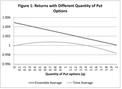
observations. I report the ensemble and time averages for each value of q in Figure 1.

Figure 1 shows the ensemble and time averages for different quantities of put options. I

find that the ensemble average of returns is always decreasing in quantity of put option, which

suggests an investor should not buy any put options. In contrast, the time average of returns has

a convex shape over quantity, which suggests an investor should buy a positive quantity of

options. In particular, the optimal quantity for the time average in Figure 1 is approximately

0.70. Interestingly, this is similar to the optimal quantity identified under the log utility in Bell

(2014).

Although the particular risk management model that I analyze here is unique, the results

confirm some of the stylized facts from Peters’ research. For example: the linear shape of the

ensemble average, the non-linear shape of the time average, and the fact that the time average

leads to more prudent behaviour than the ensemble average. These results are encouraging for

my model and the topic area.

0.996 0.998 1 1.002 1.004 1.006

0

[image:6.612.103.513.142.442.2]

0.1 0.2 0.3 0.4 0.5 0.6 0.7 0.8 0.9 1 1.1 1.2 1.3 1.4 1.5 1.6 1.7 1.8 1.9 2 Quantity of Put options (q)

Figure 1: Returns with Different Quantity of Put

Options

(7)

It is important to explore how results change with different sample sizes because it can

provide insight into the stability or robustness of the distribution of returns and statistics of the

distribution. In what follows, I refer to the optimal quantity as that which maximizes the time

average of returns. I do not consider the ensemble average because the optimal quantity is

generally a corner solution and the time average is the controversial new concept that deserves

attention.

I explore properties of the optimal quantity using a standard resampling procedure. I

specify the sample size and then conduct the optimization exercise 100,000 different times. Each

time I identify an estimate of the optimal quantity. By repeating this exercise with different

sample sizes, I establish properties of the time average in small samples. I use sample sizes

equal to 100, 1,000, 10,000, and 100,000. For each sample size, I report the distribution of the

location of the optimal quantity for a truncated set of q in Table 1.

Table 1: Frequency of Optimal Quantity for Different Sample Sizes

0.00 0.20 0.40 0.60 0.80 1.00 1.20

100 0.41 0.04 0.04 0.04 0.03 0.04 0.41

1,000 0.14 0.09 0.12 0.14 0.13 0.14 0.24

10,000 0.00 0.01 0.11 0.34 0.38 0.14 0.02

100,000 0.00 0.00 0.00 0.38 0.62 0.00 0.00

The columns in Table 1 represent intervals for the quantity of put options. The values in

the columns represent midpoints for the intervals. The rows represent the sample sizes. The

bottom row in Table 1 represents the results for a large sample, which are concentrated around

the optimal quantity (between the 0.60 and 0.80 columns). The results for large sample have

limited variability. The results in the top row of Table 1 represent a small sample and show large

variability. A corner solution (q*=0 or q*1.2) is very common with small samples, and the

large-sample optimum occurs infrequently. This raises some concerns about the behaviour of the

(8)

The analysis so far has focused on two different measures for the first moment of returns,

but what about higher moments? Higher moments reflect important information about the

distribution of returns and I am keen to raise the topic in relation to Peters’ work. To help bring

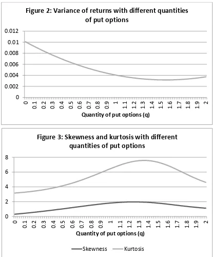
attention to these moments, I show the variance, skewness, and excess kurtosis for different

quantities of options.

0 0.002 0.004 0.006 0.008 0.01 0.012

0

[image:8.612.97.512.212.712.2]

0.1 0.2 0.3 0.4 0.5 0.6 0.7 0.8 0.9 1 1.1 1.2 1.3 1.4 1.5 1.6 1.7 1.8 1.9 2 Quantity of put options (q)

Figure 2: Variance of returns with different quantities

of put options

0 2 4 6 8

0

0.1 0.2 0.3 0.4 0.5 0.6 0.7 0.8 0.9 1 1.1 1.2 1.3 1.4 1.5 1.6 1.7 1.8 1.9 2 Quantity of put options (q)

Figure 3: Skewness and kurtosis with different

quantities of put options

(9)

different quantities of put options. It seems that there is a sweet spot with low variance, positive

skewness, and positive kurtosis in a region around q=1.4. This combination of higher moments

is desirable because it is associated with large, positive returns. It is also quite close to the

optimal quantity (q=1.57) identified under the mean-variance utility function in Bell (2014).

However, this region is quite far from the optimal quantity associated with the time average in

large samples.

Conclusion

This short paper demonstrates the use of the time average for risk management in a

simulation setting. In a large sample setting, I show that the ensemble average decreases linearly

with the quantity of put options, whereas the time average has a convex shape. These different

shapes lead to very different risk management behaviour, which concur with stylized facts

reported in work by Ole Peters (see Towers Watson, 2012).

In the second section of the paper I use resampling techniques to show how the

distribution of the optimal quantity associated with the time average of returns changes with

different sample sizes. For small sample sizes (100 or 1,000), I find large variability in the

optimal quantity. For larger sample sizes (10,000 or 100,000), I find the optimal quantity is

densely concentrated around the optimal quantity. These results raises concerns about behaviour

of the time average in small samples, but suggest the statistic is well behaved in large samples.

In the third section of the paper I show higher moments of the distribution for returns in a

large sample setting. I find that a region around q=1.4 is associated with low variance, positive

skewness, and kurtosis for returns, which are desirable qualities for the distribution of returns. It

is not clear to me how these higher moments are related to the discussion of the time average and

I hope to draw attention to this matter by presenting these results here.

I use geometric Brownian motion to represent the stock price in this paper because this

model is directly analogous to the stochastic differential equations used in Peters’ work.

However, Brownian motion is sometimes referred to as mild randomness and I am keen to

extend the simulations conducted here to so-called wild types of randomness in the future, such

(10)

Bell, P. (2014). Optimal use of put options in a stock portfolio. Unpublished manuscript.

Available from http://mpra.ub.uni-muenchen.de/54871/

Calvet, L. & Fisher, A. (2002). Multifractality in asset returns: theory and evidence. The

Review of Economics and Statistics, 84, 381-406.

Peters, O. (2010). Optimal leverage from non-ergodicity. Quantitative Finance, 11(11),

1593-1602.

Peters, O. (2011a). The time resolution of the St. Petersburg paradox. Philosophical

Transactions of the Royal Society A: Mathematical, Physical and Engineering Sciences,

369(1956), 4913-4931.

Peters, O. (2011b). Menger 1934 Revisited. Manuscript submitted for publication. Available

from http://arxiv.org/abs/1110.1578.

Peters, O. & Gell-Mann, M. (2014). Evaluating gambles using dynamics. Manuscript submitted

for publication. Available from http://arxiv.org/abs/1405.0585.

Towers Watson. (2012). The irreversibility of time: Or why you should not listen to financial

economists. London, UK: Ole Peters.

Wengert, C. (2010). Multifractal Model of Asset Returns (MMAR) [Software]. Available from

(11)

%% Code Appendix -- Properties of Returns Distributions % Written by Peter Bell, May 5 2014

% %

%% Section 1: Specify global parameters for stock and put option. %

clear all;

S=100; K=100; mu=0; sig=0.10;

d1=(1/sig)*(log(S/K)+0.5*sig^2); d2 = d1 - sig; P = K*normcdf(-d2,0,1)-S*normcdf(-d1,0,1);

%% Section 2: Simulate results in large sample %

LargeN=10^5;

s = RandStream.create('mt19937ar','seed',5489);

RandStream.setDefaultStream(s); z=mu+sig*randn(LargeN,1);

S1=S.*exp(z); Pr=zeros(1,1);

for i=1:101

Q=(i-1)/50; P1=Q*(max(K-S1,0)-P); Pr(i,1:LargeN)=(S1+P1)/100; Stats(i,1)=mean(Pr(i,1:LargeN)); Stats(i,2)=geomean(Pr(i,1:LargeN)); Stats(i,3)=var(Pr(i,1:LargeN)); Stats(i,4)=skewness(Pr(i,1:LargeN)); Stats(i,5)=kurtosis(Pr(i,1:LargeN)); end

%% Section 3: Simulate results with resampling

% Please repeat this section and hard-code changes to the following % variable... VarN=10^2, 10^3, 10^4, and 10^5.

%

VarN=10^2; ResampN=10^5; MaxQ=zeros(1,1);

for j=1:ResampN

z=mu+sig*randn(VarN,1); S1=S.*exp(z);

Pr=zeros(1,1);

for i=1:101

Q=(i-1)/50;

P1=Q*(max(K-S1,0)-P); Pr(i,1:VarN)=(S1+P1)/100;

GeomAvg(i,j)=geomean(Pr(i,1:VarN)); end

[rMax iMax] = max(GeomAvg(:,j)); MaxQ(j,1)=(iMax-1)/50;

end

histIndexTwo = 0:0.2:1.2;

[qStarHistLog xOut] = hist(MaxQ(:,1), histIndexTwo);