Comparison of different feature sets for identification of variants in progressive aphasia

Comparison of different feature sets for identification of variants in

progressive aphasia

Kathleen C. Fraser1_{, Graeme Hirst}1_{, Naida L. Graham}2_{, Jed A. Meltzer}3_,

Sandra E. Black4_{, and Elizabeth Rochon}2 1_{Dept. of Computer Science, University of Toronto}

2_{Dept. of Speech-Language Pathology, University of Toronto, & Toronto Rehabilitation Institute} 3_{Rotman Research Institute, Baycrest Centre, Toronto}

4_{LC Campbell Cognitive Neurology Research Unit, Sunnybrook Health Sciences Centre, Toronto} {kfraser,gh}@cs.toronto.edu, {naida.graham,elizabeth.rochon}@utoronto.ca

[email protected], [email protected] Abstract

We use computational techniques to ex-tract a large number of different features from the narrative speech of individuals with primary progressive aphasia (PPA). We examine several different types of fea-tures, including part-of-speech, complex-ity, context-free grammar, fluency, psy-cholinguistic, vocabulary richness, and acoustic, and discuss the circumstances under which they can be extracted. We consider the task of training a machine learning classifier to determine whether a participant is a control, or has the fluent or nonfluent variant of PPA. We first evaluate the individual feature sets on their classifi-cation accuracy, then perform an ablation study to determine the optimal combina-tion of feature sets. Finally, we rank the features in four practical scenarios: given audio data only, given unsegmented tran-scripts only, given segmented trantran-scripts only, and given both audio and segmented transcripts. We find that psycholinguis-tic features are highly discriminative in most cases, and that acoustic, context-free grammar, and part-of-speech features can also be important in some circumstances.

1 Introduction

In some types of dementia, such as primary pro-gressive aphasia, language deficit is a core symp-tom, and the analysis of narrative or conversa-tional speech is important for assessing the extent of an individual’s language impairment. Analy-sis of connected speech has been limited in the past because it is time-consuming and requires ex-pert annotation. However, studies have shown that it is possible for machine learning classifiers to achieve high accuracy on some diagnostic tasks

when trained on features which were automati-cally extracted from speech transcripts.

In this paper, we summarize previous research on the automatic analysis of speech samples from individuals with dementia, focusing in particular on primary progressive aphasia. We discuss in de-tail different types of features and compare their effectiveness in the classification task. We sug-gest some benefits and drawbacks of these differ-ent features. We also examine the interactions be-tween different feature sets, and discuss the rela-tive importance of individual features across fea-ture sets. Because we examine a large number of features on a relatively small data set, we em-phasize that this work is exploratory in nature; nonetheless, our results are consistent with, and extend, previous work in the field.

2 Background

In recent years, there has been growing interest in using computer techniques to automatically detect dementia from speech and language features de-rived from a sample of narrative speech. Some re-searchers have explored ways to use methods such as part-of-speech tagging, statistical parsing, and speech signal analysis to detect disorders such as dementia of the Alzheimer’s type (DAT) (Bucks et al., 2000; Singh et al., 2001; Thomas et al., 2005; Jarrold et al., 2010) and mild cognitive impairment (MCI) (Roark et al., 2011).

Here, we focus on a type of dementia called primary progressive aphasia (PPA). PPA is a sub-type of frontotemporal dementia (FTD) which is characterized by progressive language impairment without other notable cognitive impairment. There are three subtypes of PPA: semantic dementia (SD), progressive nonfluent aphasia (PNFA), and logopenic progressive aphasia (LPA). SD, some-times called “fluent” progressive aphasia, is typi-cally marked by fluent but empty speech, anomia,

deficits in comprehension, and spared grammar and syntax (Gorno-Tempini et al., 2011). In contrast, PNFA is characterized by halting and sometimes agrammatic speech, reduced syntac-tic complexity, word-finding difficulties, and rela-tively spared single-word comprehension (Gorno-Tempini et al., 2011). The third subtype, LPA, is characterized by slow speech and frequent word finding difficulties; this subtype is not included in the current analysis.

Although clear diagnostic criteria for PPA have been established (Gorno-Tempini et al., 2011), there is no one test which can provide a diagno-sis. Classification of PPA into subtypes requires evaluation of spoken output, as well as neuropsy-chological assessment and brain imaging. Quali-tative evaluation of speech often can be done accu-rately by clinicians or researchers, but the ability to do this evaluation can require years of training and experience. Some researchers have performed detailed quantitative characterization of speech in PPA, but the precise characteristics of speech are not yet fully understood and this process is too time-consuming for most clinicians.

Peintner et al. (2008) conducted one of the earli-est automatic analyses of speech from individuals with FTD, including SD and PNFA as well as a behavioural variant. They considered psycholin-guistic features as well as phoneme duration fea-tures extracted from the audio samples. Although they were fairly successful in classifying partici-pants according to their subtype, they did not re-port many details regarding the specific features which were useful or how those features might re-flect the underlying impairment of the speakers.

Pakhomov et al. (2010a) examined FTD speech from an information-theoretic approach. They constructed a language model of healthy control speech, and then calculated the perplexity and out-of-vocabulary rate for each of the patient groups relative to that model. In another study, Pakhomov et al. (2010b) extracted speech and language fea-tures from samples of FTD speech. In a principal components analysis, they discovered four com-ponents which accounted for most of the variance in their data: speech length, hesitancy, empty con-tent, and grammaticality. However, they did not perform any classification experiments.

Fraser et al. (2013a) attempted to classify par-ticipants as either SD patients, PNFA patients, or healthy controls using a large number of language

SD

(N=11) PNFA(N=13) Control(N=16)

Male/Female 8/3 7/6 9/7

Age (yrs) 65.9 (7.1) 64.5 (10.4) 67.8 (8.2) Education (yrs) 17.5 (5.8) 14.0 (3.5) 16.8 (4.3)

Table 1: Demographic information. Numbers are given in the form: mean (standard deviation).

features extracted from manually-transcribed tran-scripts. They distinguished between SD and con-trol participants with very high accuracy, and were also successful at distinguishing between PNFA and control participants. However, their method did not perform as well on the task of classify-ing SD vs. PNFA speakers. In subsequent work (Fraser et al., 2013b), they expanded their feature set to include acoustic features extracted directly from the audio file.

3 Methods 3.1 Data

Twenty-four patients with PPA were recruited through three Toronto memory clinics, and 16 age-and education-matched healthy controls were re-cruited through a volunteer pool. All participants were native speakers of English, or had completed some of their education in English. Exclusion cri-teria included a known history of drug or alcohol abuse and a history of neurological or major psy-chiatric illness. Each patient was diagnosed by a behavioural neurologist and all met current crite-ria for PPA (Gorno-Tempini et al., 2011). Table 1 shows demographic information for each group.

To elicit a sample of narrative speech, partici-pants were asked to tell the well-known story of Cinderella. They were given a wordless picture book to remind them of the story; then the book was removed and they were asked to tell the story in their own words. This procedure, described in full by Saffran et al. (1989), is commonly used in studies of connected speech in aphasia.

The narrative samples were transcribed by trained research assistants. The transcriptions in-clude filled pauses, repetitions, and false starts, and were annotated with the total speech time. Sentence boundaries were marked according to se-mantic, syntactic, and prosodic cues.

3.2 Classification framework

and use them to train a support vector machine (SVM) classifier. We use a leave-one-out cross-validation framework and report the average ac-curacy (i.e. proportion of correctly classified in-stances) across folds. We optimize the complexity parameter and the kernel type in a nested cross-validation loop over the training set. For compar-ison, we also tested a na¨ıve Bayes classifier; how-ever we found that the results were consistently poorer and we do not report them here.

3.3 Features

In the following sections we will describe each of the feature sets that we use and explain how the features are computed, and we will discuss some of the potential advantages and disadvantages as-sociated with each set. In particular, we discuss what types of data are necessary for the extraction of these features. The data types are: unsegmented transcripts, segmented transcripts, and audio.

3.3.1 Part-of-speech features

Different categories of words may be selectively impaired in different types of dementia. In PPA, individuals with SD tend to be more impaired with respect to nouns than verbs, and may replace nouns with pronouns or circumlocutory phrases. In contrast, individuals with PNFA may have more difficulty with verbs and may even demonstrate agrammatism, which can result in the omission of grammatical morphemes and function words. Thus, it is often useful to compare the relative fre-quencies with which words representing the differ-ent parts-of-speech (POS) are produced in a sam-ple, as in Table 2. Similar features have been re-ported in computational studies of MCI (Roark et al., 2011), FTD (Pakhomov et al., 2010b), and DAT (Bucks et al., 2000). Numerous POS taggers exist, although we use the Stanford tagger here (Toutanova et al., 2003).

3.3.2 Complexity features

Changes in linguistic complexity may accompany the onset of dementia, although some studies have found a decrease in complexity (e.g. Kemper et al. (2001)) while others have found an increase (e.g. Le et al. (2011)).

The features in Table 3 vary in their ease of computation. Mean word length can be calculated from an unsegmented transcript, while mean sen-tence length requires only sensen-tence boundary seg-mentation. Other measures, such as Yngve depth

Nouns # nouns / # words Verbs # verbs / # words

Noun-verb ratio # nouns / # verbs Noun ratio # nouns / (# nouns + # verbs) Inflected verbs # inflected verbs / # verbs Determiners # determiners / # words Demonstratives # demonstratives / # words Prepositions # prepositions / # words Adjectives # adjectives / # words Adverbs # adverbs / # words

Pronoun ratio # pronouns / (# nouns + # pronouns) Function words # function words / # words Interjections # interjections / # words

Table 2: Part-of-speech features.

Max depth maximum Yngve depth of each parse tree, averaged over all sentences

Mean depth mean Yngve depth of each node in the parse tree, averaged over all sentences Total depthtotal sum of the Yngve depths of each node

in the parse tree, averaged over all sentences Tree height height of each parse tree, averaged over

all sentences

MLS mean length of sentence MLC mean length of clause MLT mean length of T-unit

Subordinate conjunctions number of subordinate conjunctions

Coordinate conjunctions number of coordinate con-junctions

Subordinate:coordinate ratio ratio of number of sub-ordinate conjunctions to number of cosub-ordinate conjunctions

Mean word length mean length, in letters, of each word in the sample

Table 3: Complexity features.

(Yngve, 1960), require full parses of the sentences (we use the Stanford parser (Klein and Manning, 2003) and Lu’s Syntactic Complexity Analyzer (Lu, 2010)).

3.3.3 CFG features

Although many of the complexity features above are derived from parse trees, in this section we present a set of features that take into account the context-free grammar (CFG) labels on each of the nodes. CFG features have been previously used to assess the grammaticality of sentences in an artificial error corpus (Wong and Dras, 2010) and to distinguish human from machine transla-tions (Chae and Nenkova, 2009). However, this is the first time such features have been applied to speech from participants with dementia.

NP→NNSNoun phrases consisting of only a plural noun

VP → VBN PP Verb phrases consisting of a past-participle verb and a prepositional phrase ROOT→INTJ Trees consisting of only an

interjec-tion

Phrase type proportion Length of each phrase type (noun phrase, verb phrase, or prepositional phrase), divided by total narrative length Average phrase type length Total number of words in

a phrase type, divided by the number of phrases of that type

Phrase type rate Number of phrases of a given type, divided by total narrative length

Table 4: CFG features.

Um Frequency of filled pauseum

Uh Frequency of filled pauseuh

NID Frequency of words Not In Dictionary (e.g. para-phasias, neologisms)

Verbal rate Number of words per minute Total words Total number of words produced

Table 5: Fluency features.

3.3.4 Fluency features

Park et al. (2011) found that listeners’ judgements of fluency were affected by a number of different variables, and the three most discriminative fea-tures were “speech rate, speech productivity, and audible struggle.” For our list of fluency features (Table 5), we include only those features which could be extracted from the transcripts alone (as-suming the total speech time is given). We count pauses filled byumanduhseparately, as research has suggested that they may indicate different cog-nitive processes (Clark and Fox Tree, 2002).

The number of words in a sample could be eas-ily generated using the word count feature in most text-editing software (although we first exclude filled pauses and NID tokens), and the verbal rate can subsequently be calculated directly. The other three features are easily calculated using string matching and an electronic dictionary.

3.3.5 Psycholinguistic features

Some types of dementia are characterized by im-pairments in semantic access. Such imim-pairments may be sensitive to psycholinguistic features such as lexical frequency, familiarity, imageability, and age of acquisition (Table 6). We use the SUBTL frequency norms (Brysbaert and New, 2009) and the combined Bristol and Gilhooly-Logie norms (Stadthagen-Gonzalez and Davis, 2006; Gilhooly and Logie, 1980) for familiarity, imageability, and

Frequency Frequency with which a word occurs in some corpus of natural language

Familiarity Subjective rating of how familiar a word seems

Imageability Subjective rating of how easily a word generates an image in the mind

Age of acquisition Subjective rating of how old a per-son is when they first learn that word

Light verbs Number of occurrences ofbe,have,come,

go, give, take, make, do, get, move, andput, normalized by total number of verbs

Table 6: Psycholinguistic features.

age of acquisition (see Table 6). We compute the average of each of these measures for all content words, as well as for nouns and verbs separately.

Another measure that fits into this category is the frequency of occurrence of light verbs, which an impaired speaker may use to replace a more specific verb. We use the same list of light verbs as Breedin et al. (1998), given in Table 6.

One challenge associated with psycholinguis-tic features is finding norms which provide ade-quate coverage for the given data. Fraser et al. (2013a) reported that the SUBTL frequency norms had a coverage of above 90% on their data, but the Bristol-Gilhooly-Logie norms had a coverage of only around 30%.

3.3.6 Vocabulary richness features

Individuals experiencing semantic difficulty may use a limited range of vocabulary. We can mea-sure the vocabulary richness or lexical diversity of a narrative sample using a number of different metrics (see Table 7). Type-token ratio has been a popular choice, perhaps due to its simplicity; however it is sensitive to the length of the sample. Bucks et al. (2000) were the first to apply Honor´e’s statistic and Brun´et’s index to the study of demen-tia, and found significant differences between in-dividuals with DAT and healthy controls. Cov-ington and McFall (2010) proposed a new mea-sure called the moving-average type-token ratio (MATTR), which is independent of text length. This feature was later applied to aphasic speech in a study by Fergadiotis and Wright (2011), and was found to be one of the most unbiased indicators of lexical diversity in impaired speakers.

Honor´e’s statistic NV−0.165

/whereVis the number of word types andNis the number of word tokens. Brun´et’s index 100logN/(1−V1/V)whereV1is the

number of words used only once,V is the total number of word types, andNis the number of word tokens.

Type-token ratio (TTR) V/N whereV is the num-ber of word types andNis the number of word tokens.

Moving-average type-token ratio (MATTRw) TTR calculated over a moving window of size w, and averaged over all windows.

Table 7: Vocabulary richness features.

3.3.7 Acoustic features

What we call acoustic features are extracted di-rectly from the audio file. We consider the fea-tures given in Table 8. Acoustic feafea-tures have been shown to be useful when automatically detecting conditions such as Parkinson’s disease, in which changes in speech are common (Little et al., 2009; Tsanas et al., 2012). Acoustic features have also been examined in studies of DAT (Meil´an et al., 2014), FTD (Pakhomov et al., 2010b), and PPA (Fraser et al., 2013b, whose software we use here). An obvious benefit to acoustic features is that they do not require a transcription, and can be cal-culated immediately given an audio sample. The corresponding drawback is that they tell us noth-ing about the lnoth-inguistic content of the narrative.

4 Experiments

We report the results of three experiments explor-ing the discriminative power of the different fea-tures. We first compare the classification accura-cies using each individual feature set. We then per-form an ablation study to determine which com-bination of feature sets leads to the highest clas-sification accuracy. We also look at individual features across sets and discuss which ones are the most discriminative, particularly in situations where data might be limited.

4.1 Individual comparison of accuracy by set

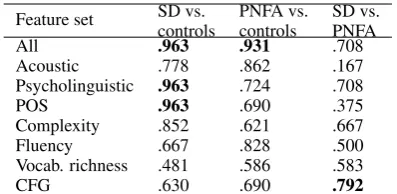
The accuracies which result from using each fea-ture set individually are given in Table 9. The highest accuracy across the three tasks is achieved in distinguishing SD participants from controls. An accuracy of .963 can be achieved using all the features together, or using the psycholinguis-tic or POS features alone. This is consistent with the semantic impairments that are observed in SD.

Total duration of speech Total length of all non-silent segments

Phonation rate Total duration of speech / total dura-tion of the sample (including pauses)

Mean pause duration Mean length of pauses>0.15 ms

Short pause count # Pauses>0.15 ms and<0.4 ms Long pause count # Pauses>0.4 ms

Pause:word ratio Ratio of silent segments longer than 150 ms to non-silent segments

F0:3mean Mean of the fundamental frequency and the

first three formant frequencies

F0:3variance Variance of the fundamental frequency

and the first three formant frequencies Mean instantaneous power Measure related to the

loudness of the signal

Mean 1st ACFMean first autocorrelation function Max 1st ACFMaximum first autocorrelation function Skewness Measure of lack of symmetry, associated

with tense or creaky voice

Kurtosis Measure of the peakedness of the signal ZCR Zero-crossing rate, can be used to distinguish

between voiced and unvoiced regions

MRPDE Mean recurrence period density entropy, a measure of periodicity

Jitter Measure of the short-term variation in the pitch (frequency) of a voice

Shimmer Measure of the short-term variation in the loudness (amplitude) of a voice

Table 8: Acoustic features.

The measures of vocabulary richness do not distin-guish between the SD and control groups, suggest-ing it is the words themselves, and not the number of different words being used, that is important.

In the case of PNFA participants vs. controls, we find that the highest accuracy is achieved ing all the features, and the second highest by us-ing only acoustic features. This is not surprisus-ing, considering that the acoustic features include mea-sures of pausing and phonation rate, which can detect the characteristic halting speech of PNFA. The third best accuracy is achieved using the flu-ency features, which also fits with this explana-tion. However, we might have expected that the complexity and CFG features would be more sen-sitive to the grammatical impairments of PNFA.

fea-Feature set SD vs._controls PNFA vs._controls SD vs._PNFA

All .963 .931 .708

Acoustic .778 .862 .167

Psycholinguistic .963 .724 .708

POS .963 .690 .375

Complexity .852 .621 .667

Fluency .667 .828 .500

Vocab. richness .481 .586 .583

CFG .630 .690 .792

Table 9: Classification accuracies for each feature set individually using a SVM classifier. Bold indi-cates the highest accuracy for each task.

tures are actually higher than the results using all features. This demonstrates that classifier perfor-mance can be adversely affected by the presence of irrelevant features, especially in small data sets.

4.2 Combining feature sets

In the previous section we examined the feature sets individually; however, one type of feature may complement the information contained in an-other feature set, or it may contain redundant in-formation. To examine the interactions between the feature sets, we perform an ablation study. Starting with all the features, we remove each fea-ture set one at a time and measure the accuracy of the classifier. The feature set whose removal causes the smallest decrease in accuracy is then re-moved permanently from the experiment, the rea-soning being that the most important feature sets will cause the greatest decrease in accuracy when removed. In some cases, we observe that the clas-sification accuracy actually increases when a set is removed, which suggests that those features are not relevant to the classification (at least in combi-nation with the other sets). In the case of a tie, we remove the feature set whose individual classifica-tion accuracy on that task is lowest. The procedure is then repeated on the remaining feature sets, con-tinuing until only one set remains.

The results for SD vs. controls are given in Ta-ble 10a. The best result, 1.00, is achieved by combining the psycholinguistic and POS features. This is unsurprising, since each of those feature sets perform well individually. Curiously, the same result can also be achieved by also including the complexity, vocabulary richness, and CFG fea-tures, but not in the intermediate stages between those two optimal sets. We attribute this to the in-teractions between features and the small data set. For PNFA vs. controls, shown in Table 10b, the

(a) SD vs. controls.

Removed Remaining Features Accuracy A+P+POS+C+F+VR+CFG .963

F A+P+POS+C+VR+CFG .963

A P+POS+C+VR+CFG 1.00

VR P+POS+C+CFG .926

CFG P+POS+C .926

C P+POS 1.00

POS P .963

(b) PNFA vs. controls.

Removed Remaining Features Accuracy A+P+POS+C+F+VR+CFG .931

VR A+P+POS+C+F+CFG .931

C A+P+POS+F+CFG .931

POS A+P+F+CFG .931

CFG A+P+F .966

F A+P .966

P A .862

(c) SD vs. PNFA.

Removed Remaining Features Accuracy A+P+POS+C+F+VR+CFG .708

POS A+P+C+F+VR+CFG .750

VR A+P+C+F+CFG .833

F A+P+C+CFG .833

A P+C+CFG .792

C P+CFG .917

P CFG .792

Table 10: A=acoustic, P=psycholinguistic, POS=part-of-speech, C=complexity, F=fluency, VR=vocabulary richness, CFG=CFG production rule features. Bold indicates the highest accuracy with the fewest feature sets.

best result of .966 is achieved using a combina-tion of acoustic and psycholinguistic features. In this case the removal of the fluency features, which gave the second highest individual accuracy, does not make a difference to the accuracy. This sug-gests that the fluency features contain similar in-formation to one of the remaining sets, presum-ably the acoustic set.

In the case of SD vs. PNFA, we again see that the best accuracy can be achieved by combining two feature sets, as shown in Table 10c. Us-ing psycholUs-inguistic and CFG features, we can achieve an accuracy of .917, a substantial im-provement over the best accuracy for this task in Table 9. In fact, in all three cases we see that us-ing a carefully selected combination of feature sets can result in better accuracy than using all the fea-ture sets together or using any one set individually.

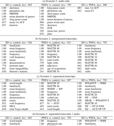
4.3 Best features for incomplete data

features are the most discriminative across feature sets. We approach this as a practical consideration: given the data that a researcher has, and limited re-sources, what are the best features to measure? We consider the following four scenarios:

1. Given audio files only. This scenario often arises because it is relatively easy to record speech, but difficult to have it transcribed. Only acoustic features can be extracted. 2. Given basic transcriptions only (no audio).

We assume there is no sentence segmentation and the time is not marked (e.g. as in the out-put of automatic speech recognition). Thus, we can measure psycholinguistic, POS, and vocabulary measures. We can also measure the fluency features except for verbal rate, as well as mean word length and subordi-nate/coordinate conjunctions from the com-plexity set. Without sentence boundaries, we cannot parse the transcripts.

3. Given fully segmented transcripts (no audio). We can measure all features except for acous-tic features.

4. Given audio and fully segmented transcripts. We can measure all features.

For each scenario, we rank the available fea-tures by theirχ2_{value and choose the top 10 only}

as input to the SVM classifier (see Manning et al. (2008) for a complete explanation ofχ2_feature

se-lection). We only include features ifχ2_{>0, so in}

cases where there are very few relevant features, fewer than 10 features may be selected. Because we perform cross-validation, the selected features may vary across different folds. In the tables that follow, we present the features ranked by the num-ber of folds in which they appear (i.e. a feature with the value 1.00 was selected in every fold). Due to space constraints, only the top 10 ranked features are shown.

The results for Scenario 1 are given in Ta-ble 11a. For the SD vs. controls and PNFA vs. controls, the most highly ranked features tend to be related to fluency and rate of speech, as well as voice quality (skewness and MRPDE). How-ever, when distinguishing between the two patient groups, the acoustic features are essentially use-less. In most cases, we see thatnoneof the acous-tic features had a non-zeroχ2_{value, and thus the}

classifier could not be properly trained.

For Scenario 2 (Table 11b), the results for SD vs. controls show that within the psycholinguistic

and POS feature sets, features relating to familiar-ity and frequency are very important, as well as nouns and demonstratives. In the PNFA vs. con-trols case, we see that a number of the vocabulary richness features are selected, which is in contrast to the previous two experiments. However, it ap-pears that only the MATTR feature is important (with varying window lengths), so when we con-sidered only full feature sets, that information was obscured by the other, irrelevant features in that set. The SD vs. PNFA case shows a mix of fea-tures from the previous two cases.

For Scenario 3 (Table 11c), we add the com-plexity and CFG features. These features do not have a large effect in the SD vs. controls case, but a few CFG features are selected in the PNFA vs. controls and SD vs. PNFA cases.

In Scenario 4 (Table 11d), we consider all fea-tures. In the SD vs. controls case this increases the accuracy. However, for PNFA vs. controls and SD vs. PNFA, the classification accuracy actually decreases, relative to Scenario 3. When the num-ber of features increases, the potential to overfit to the training data fold also increases, and it seems likely that that is occurring here. Nonetheless, we expect that the features which are selected in every fold are still highly relevant. These features are unchanged between Scenarios 3 and 4 in the SD vs. controls and SD vs. PNFA case, however in the PNFA vs. controls case, the acoustic features are now ranked more highly than some of the vocabu-lary richness and CFG features from Scenario 3.

5 Discussion

While it may be tempting to calculate as many features as possible and use them all in a classi-fier, we have shown here that better results can be achieved by choosing a small, relevant subset of features. In particular, psycholinguistic features such as frequency and familiarity were useful in all three classification tasks. Acoustic features were useful in discriminating patients from controls, but not for discriminating between the two PPA sub-types. We also found that MATTR was relevant in some cases, although the other vocabulary rich-ness features were not, and that the CFG features were more useful than traditional measures of syn-tactic complexity. POS features were useful only in distinguishing between SD and controls.

(a) Scenario 1: audio only.

SD vs. control, Acc: .852 PNFA vs. control, Acc: .793 SD vs. PNFA, Acc: .500

1.00 skewness 1.00 long pause count .083 max 1st ACF

1.00 phonation rate 1.00 phonation rate .042 mean F3

1.00 MRPDE 1.00 short pause count

1.00 mean duration of pauses 1.00 MRPDE

.037 long pause count 1.00 mean duration of pauses .037 mean 1st ACF .966 pause:word ratio

.037 kurtosis .793 skewness

.793 ZCR

.345 mean inst. power .035 jitter

(b) Scenario 2: unsegmented transcripts.

SD vs. control, Acc: .926 PNFA vs. control, Acc: .621 SD vs. PNFA, Acc: .792

1.00 familiarity 1.00 MATTR 50 1.00 familiarity

1.00 noun frequency 1.00 MATTR 40 1.00 noun frequency

1.00 noun familiarity 1.00 MATTR 30 1.00 noun familiarity

1.00 frequency 1.00 frequency 1.00 MATTR 20

1.00 verb frequency 1.00 MATTR 20 .708 MATTR 10

1.00 nouns .931 total words .208 MATTR 30

1.00 demonstratives .759 light verbs .042 MATTR 50

.778 pronoun ratio .690 adjectives .042 MATTR 40

.667 noun imageability .241 age of acquisition .042 light verbs

.630 Honor´e’s statistic .241 MATTR 10 .042 verbs

(c) Scenario 3: segmented transcripts.

SD vs. control, Acc: .926 PNFA vs. control, Acc: .897 SD vs. PNFA, Acc: .792

1.00 word length 1.00 MATTR 50 1.00 WHADVP→WRB

1.00 familiarity 1.00 MATTR 40 1.00 familiarity

1.00 noun frequency 1.00 WHNP→WP 1.00 noun familiarity

1.00 noun familiarity 1.00 frequency 1.00 noun frequency

1.00 frequency 1.00 MATTR 20 1.00 MATTR 20

1.00 demonstratives 1.00 verbal rate 1.00 NP→NNS

.889 nouns .966 MATTR 30 1.00 SBAR→WHADVP S

.852 verb frequency .827 S1→INTJ .667 MATTR 10

.630 MLS .483 total words .500 NP→DT JJ NNS

.630 total Yngve depth .414 word length .458 SQ→AUX NP VP

(d) Scenario 4: segmented transcripts + audio.

SD vs. control, Acc: .963 PNFA vs. control, Acc: .793 SD vs. PNFA, Acc: .750

1.00 word length 1.00 frequency 1.00 WHADVP→WRB

1.00 familiarity 1.00 phonation rate 1.00 familiarity

1.00 noun frequency 1.00 MRPDE 1.00 noun familiarity

1.00 noun familiarity 1.00 verbal rate 1.00 noun frequency 1.00 frequency 1.00 mean duration of pauses 1.00 MATTR 20

1.00 demonstratives .897 MATTR 50 1.00 NP→NNS

.963 phonation rate .897 WHNP→WP 1.00 SBAR→WHADVP S

.741 verb frequency .897 MATTR 20 .625 MATTR 10

.593 nouns .690 MATTR 40 .500 NP→DT JJ NNS

.333 MLS .690 MATTR 30 .458 SQ→AUX NP VP

Table 11: Classification accuracies and top 10 features for four different data scenarios.

Psychological studies are typically on the or-der of only tens to possibly hundreds of partic-ipants, while machine learning researchers often tackle problems with thousands to millions of data points. We have chosen techniques appropriate for small data sets, but acknowledging the potential weaknesses of machine learning methods when training data are limited, these findings must be considered preliminary. However, we also believe that this is a promising approach for future

ap-plications, including automated screening for lan-guage impairment, support for clinical diagnosis, tracking severity of symptoms over time, and eval-uating therapeutic interventions.

Acknowledgments

References

Steven Bird, Ewan Klein, and Edward Loper. 2009. Natural language processing with Python. O’Reilly Media, Inc. Sarah D. Breedin, Eleanor M. Saffran, and Myrna F.

Schwartz. 1998. Semantic factors in verb retrieval: An effect of complexity.Brain and Language, 63:1–31. Marc Brysbaert and Boris New. 2009. Moving beyond

Kuˇcera and Francis: A critical evaluation of current word frequency norms and the introduction of a new and im-proved word frequency measure for American English.

Behavior Research Methods, 41(4):977–990.

R.S. Bucks, S. Singh, J.M. Cuerden, and G.K. Wilcock. 2000. Analysis of spontaneous, conversational speech in dementia of Alzheimer type: Evaluation of an objective technique for analysing lexical performance. Aphasiol-ogy, 14(1):71–91.

Jieun Chae and Ani Nenkova. 2009. Predicting the fluency of text with shallow structural features: case studies of ma-chine translation and human-written text. InProceedings of the 12th Conference of the European Chapter of the As-sociation for Computational Linguistics, pages 139–147. Association for Computational Linguistics.

Herbert H. Clark and Jean E. Fox Tree. 2002. Using uh and um in spontaneous speaking. Cognition, 84(1):73–111. Michael A. Covington and Joe D. McFall. 2010. Cutting

the Gordian knot: The moving-average type–token ratio (MATTR).Journal of Quantitative Linguistics, 17(2):94– 100.

Gerasimos Fergadiotis and Heather Harris Wright. 2011. Lexical diversity for adults with and without apha-sia across discourse elicitation tasks. Aphasiology, 25(11):1414–1430.

Kathleen C. Fraser, Jed A. Meltzer, Naida L. Graham, Carol Leonard, Graeme Hirst, Sandra E. Black, and Elizabeth Rochon. 2013a. Automated classification of primary progressive aphasia subtypes from narrative speech tran-scripts. Cortex.

Kathleen C. Fraser, Frank Rudzicz, and Elizabeth Rochon. 2013b. Using text and acoustic features to diagnose pro-gressive aphasia and its subtypes. InProceedings of Inter-speech.

K.J. Gilhooly and R.H. Logie. 1980. Age-of-acquisition, im-agery, concreteness, familiarity, and ambiguity measures for 1,944 words. Behavior Research Methods, 12:395– 427.

M.L. Gorno-Tempini, A.E. Hillis, S. Weintraub, A. Kertesz, M. Mendez, S.F. Cappa, J.M. Ogar, J.D. Rohrer, S. Black, B.F. Boeve, F. Manes, N.F. Dronkers, R. Vandenberghe, K. Rascovsky, K. Patterson, B.L. Miller, D.S. Knopman, J.R. Hodges, M.M. Mesulam, and M. Grossman. 2011. Classification of primary progressive aphasia and its vari-ants.Neurology, 76:1006–1014.

William Jarrold, Bart Peintner, Eric Yeh, Ruth Krasnow, Harold Javitz, and Gary Swan. 2010. Language ana-lytics for assessing brain health: Cognitive impairment, depression and pre-symptomatic Alzheimer’s disease. In Yiyu Yao, Ron Sun, Tomaso Poggio, Jiming Liu, Ning Zhong, and Jimmy Huang, editors,Brain Informatics, vol-ume 6334 ofLecture Notes in Computer Science, pages 299–307. Springer Berlin / Heidelberg.

Susan Kemper, Marilyn Thompson, and Janet Marquis. 2001. Longitudinal change in language production: Ef-fects of aging and dementia on grammatical complex-ity and propositional content. Psychology and Aging, 16(4):600–614.

Dan Klein and Christopher D. Manning. 2003. Accurate unlexicalized parsing. InProceedings of the 41st Meeting of the Association for Computational Linguistics, pages 423–430.

Xuan Le, Ian Lancashire, Graeme Hirst, and Regina Jokel. 2011. Longitudinal detection of dementia through lex-ical and syntactic changes in writing: a case study of three British novelists. Literary and Linguistic Comput-ing, 26(4):435–461.

Max A. Little, Patrick E. McSharry, Eric J. Hunter, Jennifer Spielman, and Lorraine O. Ramig. 2009. Suitability of dysphonia measurements for telemonitoring of Parkin-son’s disease. Biomedical Engineering, IEEE Transac-tions on, 56(4):1015–1022.

Xiaofei Lu. 2010. Automatic analysis of syntactic complex-ity in second language writing. International Journal of Corpus Linguistics, 15(4):474–496.

Christopher D. Manning, Prabhakar Raghavan, and Hinrich Sch¨utze. 2008. Introduction to Information Retrieval. Cambridge University Press.

Juan Jos´e G. Meil´an, Francisco Mart´ınez-S´anchez, Juan Carro, Dolores E. L´opez, Lymarie Millian-Morell, and Jos´e M. Arana. 2014. Speech in Alzheimer’s disease: Can temporal and acoustic parameters discriminate de-mentia? Dementia and Geriatric Cognitive Disorders, 37(5-6):327–334.

Serguei V.S. Pakhomov, Glen E. Smith, Susan Marino, An-gela Birnbaum, Neill Graff-Radford, Richard Caselli, Bradley Boeve, and David D. Knopman. 2010a. A com-puterized technique to asses language use patterns in pa-tients with frontotemporal dementia.Journal of Neurolin-guistics, 23:127–144.

S.V. Pakhomov, G.E. Smith, D. Chacon, Y. Feliciano, N. Graff-Radford, R. Caselli, and D. S. Knopman. 2010b. Computerized analysis of speech and language to identify psycholinguistic correlates of frontotemporal lobar degen-eration. Cognitive and Behavioral Neurology, 23:165– 177.

Hyejin Park, Yvonne Rogalski, Amy D. Rodriguez, Zvinka Zlatar, Michelle Benjamin, Stacy Harnish, Jeffrey Ben-nett, John C. Rosenbek, Bruce Crosson, and Jamie Reilly. 2011. Perceptual cues used by listeners to discriminate fluent from nonfluent narrative discourse. Aphasiology, 25(9):998–1015.

Bart Peintner, William Jarrold, Dimitra Vergyri, Colleen Richey, Maria Luisa Gorno Tempini, and Jennifer Ogar. 2008. Learning diagnostic models using speech and lan-guage measures. InEngineering in Medicine and Biol-ogy Society, 2008. EMBS 2008. 30th Annual International Conference of the IEEE, pages 4648–4651.

Brian Roark, Margaret Mitchell, John-Paul Hosom, Kristy Hollingshead, and Jeffery Kaye. 2011. Spoken language derived measures for detecting mild cognitive impairment.

Eleanor M. Saffran, Rita Sloan Berndt, and Myrna F. Schwartz. 1989. The quantitative analysis of agrammatic production: procedure and data. Brain and Language, 37:440–479.

Sameer Singh, Romola S. Bucks, and Joanne M. Cuerden. 2001. Evaluation of an objective technique for analysing temporal variables in DAT spontaneous speech. Aphasiol-ogy, 15(6):571–583.

Hans Stadthagen-Gonzalez and Colin J. Davis. 2006. The Bristol norms for age of acquisition, imageability, and fa-miliarity.Behavior Research Methods, 38(4):598–605. Calvin Thomas, Vlado Keselj, Nick Cercone, Kenneth

Rock-wood, and Elissa Asp. 2005. Automatic detection and rating of dementia of Alzheimer type through lexical anal-ysis of spontaneous speech. InProceedings of the IEEE International Conference on Mechatronics and Automa-tion, pages 1569–1574.

Kristina Toutanova, Dan Klein, Christopher Manning, and Yoram Singer. 2003. Feature-rich part-of-speech tagging with a cyclic dependency network. InProceedings of the 2003 Conference of the North American Chapter of the Association for Computational Linguistics: Human Lan-guage Technologies, pages 252–259.

Athanasios Tsanas, Max A. Little, Patrick E. McSharry, Jen-nifer Spielman, and Lorraine O. Ramig. 2012. Novel speech signal processing algorithms for high-accuracy classification of Parkinson’s disease. IEEE Transactions on Biomedical Engineering, 59(5):1264–1271.

Sze-Meng Jojo Wong and Mark Dras. 2010. Parser features for sentence grammaticality classification. In Proceed-ings of the Australasian Language Technology Association Workshop, pages 67–75.