Inside out : a shift in perspective for building exergy analysis

Inside out: a shift in perspective

for building exergy analysis

Valentina Bonetti

University of Strathclyde, Glasgow, UK, [email protected]

Abstract:

In many countries, our lives are lived under a roof. The indoor space is constantly growing and its thermal con-ditions are kept relatively stable, within comfort requirements, by a variety of passive strategies and mechanical systems. Despite the many energy-efficiency programmes and conservation efforts, the inevitable consequence of the rise in complexity of the built environment is its increasing energy consumption, which poses urgent sustain-ability concerns. Within this scenario, many optimisation methods are attempted in building design. Among them, exergy analysis - with its roots in thermal power plants - provides a quantification of energy quality and a deeper insight into the causes of inefficiencies. However, buildings are substantially different from machines and some fundamental aspects of their exergy analysis are controversial, such as the impact of the reference-state selection on a dynamic study, or the practical benefits of achieving high exergy efficiencies. Exergy assessments are com-plex and do not currently hold a prominent role in building design. Nonetheless, second-law approaches preserve their attractiveness and many possible methods are still unexplored. After acknowledging the thermodynamic dif-ferences between buildings and power machines and their particular aims, a simplified theoretical framework (built on the current methods) is proposed and formally compared to a state-of-the-art dynamic exergy analysis. The indoor environment is recognised as the fulcrum of all building energy interactions and the reference to assess energy quality. A case study shows the quantitative differences between the proposed idea and the classical ap-proach for the first fundamental steps of the building energy chain from the exergy demand to the emission system. Keeping the design focus on exploiting the local exergy budget, rather than minimising consumption, contributes towards flexible and low-cost sustainable buildings for integrated energy systems. Substantial further research, as-sisted by virtual representations and real-world testing, is required to explore meanings and practical implications of the proposed perspective.

Keywords:

Exergy, building, reference state, dynamic analysis, low-cost.

1. Introduction

The second law of thermodynamics originated from the study of steam engines, and current exergy methods derive from thermal plant analysis [1]. Exergy is the maximum achievable work that can be obtained by bringing the system into equilibrium with a reference environment whitout interacting with other systems [2], and it is claimed to be the quantification of energy quality. The criteria for the selection of the reference environment, which should be based on the purpose of the analysis [3], also originated from thermal plant assessments. There are at least two main problems in transferring the exergy methods from thermal plant analysis to buildings: the aim of buildings is not work production, and the processes occurring in buildings are very close to the reference state conditions and they are seldomly stationary.

The second problem of building exergy analysis is its current complexity and the high sensitivity to the reference selection when the situation is not stationary (the vast majority of the cases), which makes the chances of a wider adoption in architectural design1 fairly limited. Any way of reducing the com-plexity of dynamic analysis while preserving a reasonable correctness (in engineering terms) should be constructively evaluated. In this context, a major role is played by the reference-state choice, still a highly-controversial topic, especially in the dynamic case [6]. The ambient air temperature is generally adopted as the dynamic reference state, but some criticisms have not been resolved (for example [7]).

This study, after acknowledging the potential benefits and criticalities of building exergy analysis, attempts to overcome the two main issues expressed above by proposing a simplified theoretical framework based on the specific needs of the built environment. A different point of view that redefines the meaning of energy quality is the main proposal of this work, and only a few sample calculations are presented to convey ideas in a simple manner.

2. A reference state based on indoor comfort

In the current exergy literature, the word "cold" denotes thermal energy below the reference state temper-atureT0, and the word "warm" (or sometimes "hot") indicates a state which temperature is greater than the referenceT0 [8]. These definitions are somehow in conflict with the common use of the terms cold and warm, which refer to our thermal comfort rather than an external temperature; the original mean-ing spontaneously prevails in our mind, creatmean-ing confusion when a different interpretation is enforced. Two alternative approaches could resolve this conflict: using different words for exergy, or linking the reference state to our thermal comfort, so the terms cold and warm mantain an association with their original meaning. The main idea of this article is that adopting a fixed reference state based on indoor thermal comfort is a simple and robust selection, not only more intuitive than other choices - because it mantains the original significance of the terms warm and cold - but also convenient and relevant for building design.

Even if "thermal comfort" is not a clear-cut definition, because it depends on many variables and it is a range of conditions rather than a single value, the least diverse quantities of any building simulation model around the globe are still the thermostat set-points. In order to test the idea in a simple way, the coarsest possible definition of indoor thermal comfort is considered in this research: a dry-bulb air temperature of 20◦C for the presented winter case and 24◦C for a summer case₂.

Therefore, the proposed fixed reference stateT0,f i xed and the variable reference stateT0,variable (widely adopted in literature) under comparison in this study are respectively:

T0,f i xed =20◦C ≈ 293K, T0,variable =Tambient . (1)

The temperatureTambient is defined as the time-variant outdoor dry-bulb air temperature of the weather file used in the dynamic energy simulation software, as suggested by the current literature [6]. This article if focused on discussing the convenience of the proposed fixed reference state in a particular case study in winter conditions, but the considerations that can be deducted appear to be rather general.

1As intended by Herbert: a "synthesis of artistic and scientific creativity and invention, resulting in architectural potential for the adaptation of the environment to defined human purposes" [5].

3. Basic exergy equations

This study is focused on the exergy stored in the construction elements defining a thermal zone, the exergy carried by air flows (ventilation and ideal HVAC system) and the zone "exergy demand". Although many other exergy fluxes, such as radiative and convective exchanges of internal surfaces, can be calculated in a building, the ideas of this article are better visualised by means of these simpler quantities.

3.1. Exergy storage

The exergy stored in a portion of matter of uniform properties is expressed per unit volume by the following equation, in which the subscript n indicates a generic node:

exn= cnρn

(Tn−T0) −T0ln

Tn

T0

≈ cnρn(Tn−T0) 2

2T0

, (2)

withcnspecific heat, ρndensity andTntemperature of matter, andT0reference temperature [9]. Equation (2) is clearly positive for any value of node and reference temperatures, since any state different from the reference can theoretically produce work, but the stored exergy assumes different meanings depending on their relationship:

ifTn >T0it is called "warm exergy"; ifTn <T0it is called "cool exergy";

ifTn=T0the exergy stored is null and the node is at the reference state.

Only in order to distinguish cool and warm exergy values, the sign functionsgnis applied to (2):

exn ≈ sgn(Tn−T0) ·

cnρn(Tn−T0)2 2T0

. (3)

This is why in the graphs of Section 4 (Figures 2, 3, 4 and 5) a cool exergy is shown as negative (in blue) and a warm exergy storage appears as positive (red), even if both are actually positive. The value ofexn is then multiplied by the volume of each layer to obtain the actual storage.

3.2. Exergy of air flow and air heating or cooling systems

The exergy carried by air at a volume flow rate ofVÛ and temperatureTair, with specific heat at constant pressurecp,air and density ρair, is calculated in a similar way:

Û

E xair = cp,airρairVÛ

(Tair−T0) −T0ln

Tair

T0

. (4)

The total exergyE xairtransported in a period[t1,t2]is obtained by integrating (4) betweent1andt2.

3.3. Exergy demand

(exergy is not conserved). Instead, a "quality factor"3is associated with the energy demand derived from the energy analysis, and their product gives the exergy demand. There are different ways to define the quality factor of the energy demand of a building; in this study, the "simple" and "detailed" exergy demand expressions recommended by [6] in combination with the variable reference - as presented in 3.3.1 - are compared to the exergy demand based on the fixed reference state as presented in 3.3.2.

3.3.1. Simple and detailed exergy demand based on the variable reference

The "simple" exergy demand is calculated on the assumption that all the energy is provided at room temperature, and thus the quality factor simply results:QF = 1−T0/Tr oom, in whichT0is the recommended reference state andTr oom the indoor air temperature.

The "detailed" exergy demand, more accurate, is divided into two components: E xdem,vent is the part attributed to an ideal pre-heating of the ventilation air and the remaining partE xdem,heat is the exergy of the total loads minus the part that is preheated through the ventilation (Qdem,heat =Qdem,total−Qdem,vent)4. Each component is calculated according to:

E xdem,vent =Qdem,vent ·

1− T0

Tpr eheat −T0

lnTpr eheat

T0

, (5)

E xdem,heat = Qdem,heat·

1− T0

Tr oom

, (6)

where the reference temperatureT0is - in the dynamic case - the variable outdoor air temperature,Qdem,total andQdem,ventthe instantaneous loads andQdem,heattheir difference, andTpr eheatis the temperature at which the air is preheated.

3.3.2. Active exergy demand based on the fixed reference

If based on the fixed reference stateT0,f i xed proposed in this study, the simple exergy demand and both components of the detailed exergy demand defined in Section 3.3.1 result null. The exergy demand calculated with the fixed reference state based on comfort is null at comfort temperature by definition. This just means that the ideal minimum exergy demand of any building is zero and, in case of non-null thermal loads, the required energy is delivered reversibly at the comfort state temperature by a very large surface at a very slow rate. Quality is given by the ability of acting faster with smaller surfaces.

The definition of a heating or cooling system, even an ideal one, is needed in order to calculate a more pragmatic "active exergy demand": without an active system, the building is not actually "capable of asking" for exergy (which is the ultimate goal of bioclimatic design, where comfort is guaranteed by passive systems importing exergy from the outdoor environment). The "active exergy demand" based on the fixed reference is therefore not unique and it is dependent on the combination of the building envelope and operation with the following step of the building energy chain, the emission system, as shown in Section 4.4.2.

3The quality factor is the ratio between the exergy of a system and its energy, or, in other words, the fraction of exergy in a certain quantity of energy. It depends on the type of energy: in the case of heat exchanged at constantT for example,

QF=1−T0/T, whereT0is the reference-state temperature.

4. Case study

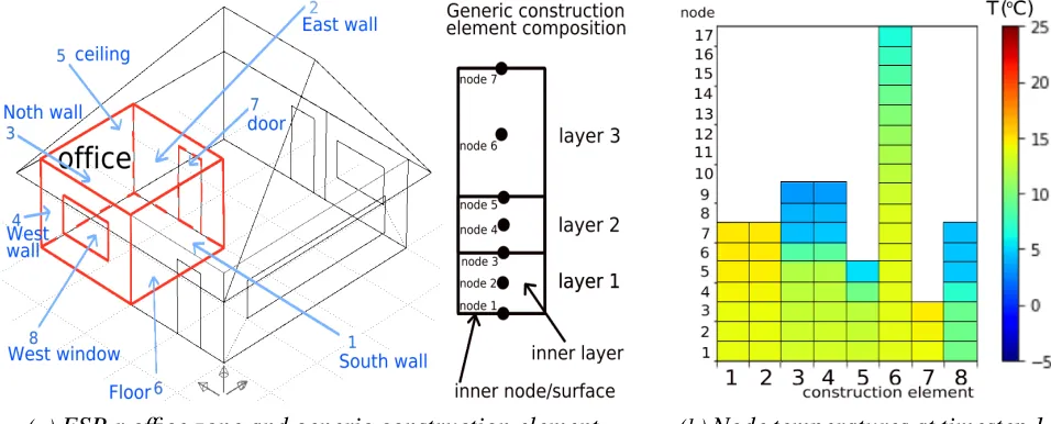
For the sake of clarity, only a limited amount of data is presented, just enough to convey the main idea of this study. The case study is a simple three-zone building, and only one zone (the office in Fig. 1) is analised. The weather file is the "default UK Climate" of the dynamic software ESP-r; three typical winter days are simulated (6th to 8th of February of the climate data) and mainly the calculations for day 3 are shown as a typical winter daily scenario.

The software ESP-r uses a finite-volume approach, which makes it possible to calculate the temperature values of nodes within constructions for each timestep. The construction elements surrounding the office zone are subdivided in a different number of layers (from one of the internal door to eight of the floor); each layer is composed of three nodes and the nodes of contiguous layer surfaces are shared. Therefore, if nlayer s is the number of layers of the particular construction element, the number of nodes for each element is 2·nlayer s +1 as shown in Fig. 1a.

(a)ESP-r office zone and generic construction element. (b)Node temperatures at timestep 1.

Fig. 1. The case study: office zone and node temperatures at first timestep; node 1 = inner surface.

The heating loads are covered by an ideal Constant Air Volume (CAV) system, with two possible settings:

maximum air temperatureTC AV,max = 30◦C and constant air rateVÛC AV =0.04m3/s; maximum air temperatureTC AV,max = 50◦C and constant air rateVÛC AV =0.02m3/s.

The CAV temperature varies up toTC AV,maxdepending on the zone loads and the air rate remains constant. The system is activated from 7am to 6pm of each day and the building is left in a free-floating mode outside of these periods.

4.1. Exergy stored in construction layers

The exergy stored in each layer of the construction elements surrounding the office zone is calculated according to (2) for each timestep. For the sake of simplicity, the central temperature of each layer (corresponding to the temperature of the central node) is used in the equation as the temperature of the entire layer. A better approach would be considering the exergy of each control volume (node) instead of the exergy stored in the entire layer and calculating the volumetric portion of each layer that is attributed to the shared interface nodes; however, for the aims of this study such accuracy is not necessary5.

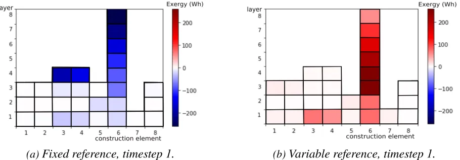
The values of exergy are highly affected by the choice of the reference state. Figure 2 shows the differences for a snapshot taken at the first timestep, which is the same timestep of the node temperatures already presented in Fig. 1b, where is easy to verify that all the nodes are below 15◦C. The exergy storage based on a fixed reference stateT0 =T0,f i xed =20◦C is classified as "cool exergy" for every node (in blue in Fig. 2a), whilst the opposite holds true for the "warm" exergy storage of Fig. 2b calculated with the variable reference, which value isT0=T0,variable[1]=2.2◦C at the first timestep.

(a)Fixed reference, timestep 1. (b)Variable reference, timestep 1.

Fig. 2. Exergy stored in construction layers (Wh), office zone.

The inner layers of the construction elements (considering here only the innermost layer for each element, numbers 1 on the bottom of the graphs in Figs.2a and 2b) interact with the indoor environment directly, and thus the exergy stored within these layers provides an idea of their dynamic behaviour and impact on indoor comfort for the next few time steps. If, for example, "cool exergy" is stored in the inner layer of a wall at the timestept∗, the layer is supposed to have a "cooling effect" on the indoor environment (providing its surface and the zone conditions allow the heat exchange) which rate and duration in time depend on the exergy quality factor and the entity of the storage. This is actually true in the case of the exergy calculated with the fixed reference state (at timestep 1 the indoor walls are below the zone temperature, so they have a cooling effect and represent a load for the heating system), but not for the exergy storage based on the variable reference: at timestep 1 cold walls are supposed to provide a "warm" contribution to the zone (because warmer than the outdoor environment), which in reality is not possible.

A qualitative idea of the trends of inner-layer exergy storage for the entire duration of the simulation is provided in Fig. 3. Figure 3a shows the exergy storage based on a fixed reference state: the inner layers of the partition walls61 and 2 have a negligible impact in terms of storage (because their temperature is very close to the reference but also because of their lightweight construction), whilst the inner layers of the rest of the constructions have a moderate cooling effect. The exergy storage based on the variable reference,

shown in Fig. 3b, tells a different story: the partition walls 1 and 2 still have an almost null impact (mainly due to their low mass construction) but the inner layers of the other elements provide a "warm storage" at every timestep, with a higher variablility (the peak value, in absolute terms, is approximately six times bigger than the one predicted by the fixed reference). Since the temperatures of the nodes of the inner layers remain below the indoor temperature for the entire period of the simulation, the fixed-reference exergy values are the ones that describe the situation as expected (cold rather than warm storage).

(a)Exergy calculated with the fixed reference (b)Exergy calculated with the variable reference

Fig. 3. Exergy stored in construction inner layers (layer 1 of each construction element), office zone.

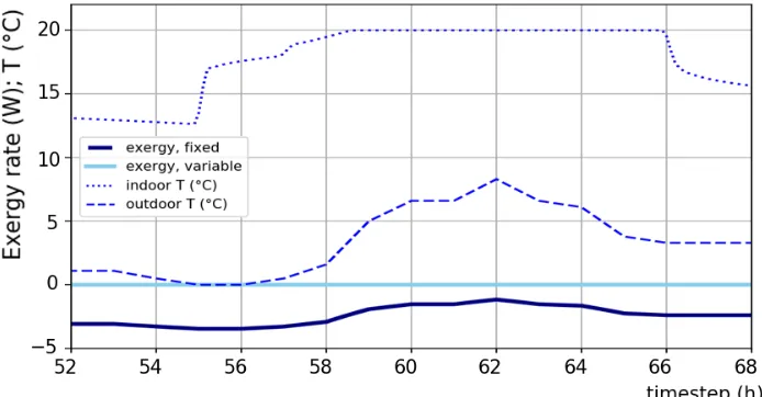
A more quantitative visualisation of the inner-envelope exergy storage is provided by the sum of all the exergy stored in the inner layers of the thermal zone for each timestep (sum of only the layers 1 of the eight construction elements). Figure 4a reports the fluctuation of the overall inner exergy storage in time for day 3 of the simulation, calculated with the fixed reference. It shows how the cool exergy stored in the envelope diminishes during the periods of active heating and internal gains (hours 55 to 66, corresponding to 7am to 6pm) and is moderately influenced by the outdoor climate (a slow cool exergy increase is observed between 00am and 7am -52h to 55h- and after 6pm, caused by the heat transfer on the outer side of the layer).

(a)Exergy calculated with the fixed reference (b)Exergy calculated with the variable reference

The values calculated with a variable reference state, reported in Fig. 4b, are instantaneously affected by the outdoor temperature: the warm exergy increases during a period when the inner layers actually become colder, only because the outdoor temperature is decreasing at a faster rate, and the entire trend shadows the outdoor temperature variations (observable in Fig. 5 of Section 4.2).

The other layers of the construction elements are obviously still important, as they determine the conditions of the inner layers and a relevant amount of their exergy will be transmitted either to the indoor or the outdoor space on the longer term. It is worth observing that the definition of "inner layer" is rather vague in this study because it just derives, for the sake of simplicity, from the geometric model subdivision of the construction elements, which does not contemplate any thermal criteria in its design [10]. A deeper effort on the definition of a more meaningful inner layer size should be made in further investigations.

4.2. Exergy of fresh air intake

Different terminology is used by different authors to indicate the outdoor air entering the zone. ESP-r defines "infiltration air" as the sum of all naturally-induced air flows and mechanical ventilation coming from outside the building, and "ventilation" the air movement between different thermal zones; various other sources use the term "ventilation" to indicate intentional intake of outdoor air and "infiltration" for unintentional fluxes of the same air. In this study, the second terminology is used because clearer to a wider audience, and thus "ventilation and infiltration" indicates the sum of all fresh air intake from the outdoor environment; the movement between zones is simply called "air from other zone".

In the case-study model, the rate of fresh air intake of the office zone (Vzone = 48m3) is fixed at 0.3 air changes per hour (ACH), which implies a volumetric flow rate of:

Û

V = ACH·Vzone/3600s =0.3·1/h·48m3· (1/3600)s/h= 0.004m3/s .

The properties of air are considered constant at cp,air = 1006 J/(kgK) and ρair = 1.2 kg/m3. These values are substituded in (4) to obtain the graph in Fig. 5.

Fig. 5. Exergy of the fresh air intake, fixed and variable reference; indoor and outdoor T (office, day 3).

4.3. Exergy of the air heating system

The heating loads of the case study are covered by the ideal Constant Air Volume (CAV) system described in Section 4, and two possible settings are explored. The exergy rate of the CAV flow is calculated with (4). The variable temperature of the heating system, CAV T, is provided by the ESP-r software and is reported in Fig. 6 for both settings. The second option, illustrated in Fig. 6b, has a higher temperature (and thus exergy factor) than the first option of Fig. 6a in every timestep, but a lower air flow rate. When the maximum temperature is lowered to 30◦C, the system is slower in reaching a comfortable indoor temperature even with a doubled air flow rate.

Since the CAV air temperature is higher than both the comfort and outdoor temperature, all the calculated exergy flows are positive, correctly representing a warm exergy contribution to the zone for both the fixed and variable reference state. If the variable reference is adopted, the system with the lowest exergy factors is particularly affected by the variation of the outdoor temperature: the variable-reference exergy line of Fig. 6a clearly mirrors the outdoor temperature trend, and a lighter mirroring effect is also visible in the case of the variable-reference curve of the higher-exergy system in Fig. 6b. These effects are not observable in the fixed-reference curves, which reflect only the CAV temperature trends.

(a)CAV T max30◦C, Const. flow rate0.04m3/s (b)CAV T max50◦C, Const. flow rate0.02m3/s

Fig. 6. Exergy flow of Constant Air Volume (CAV) system, 8th of February (day 3), office zone.

The total exergy contribution over the assessed period of day 3 ([52h,68h]) is calculated by integrating (4). The values obtained for the two CAV options are:

for the CAV with max 30◦C at constant flow rate of 0.04m3/s:

E xC AV30,f i xed = 46.47W h, E xC AV30,variable =481.1W h; for the CAV with max 50◦C at constant flow rate of 0.02m3/s:

E xC AV50,f i xed = 133.4W h, E xC AV50,variable =478.3W h.

4.4. Energy and exergy demand

Exergy calculations derive from the energy analysis. The influential terms of the daily energy balance (related to day 3 of the case study) are presented in Fig. 7a. The total heating loads and the sum of ventilation and infiltration are also shown as instantaneous values in Fig. 7b because they are required for the "detailed exergy demand" based on the variable reference state, as defined in 3.3.1. The heating-system data, required for the active exergy demand defined in 3.3.2, can be found in Section 4.3.

(a)Causal breakdown of energy balance (kWh) (b)Total heating and vent.+infiltration loads (W)

Fig. 7. Energy overall balance and detailed heating and ventilation plus infiltration loads (day 3, office).

4.4.1. Simple and detailed exergy demand based on the variable reference

The simple exergy demand defined in Section 3.3.1 is the product of the quality factor of energy at indoor air temperature Tr oom and the energy demand (in this case the total heating load of the day 3). The value must be obtained by integration, because the reference (and thus the quality factor) is the outdoor temperature, different at every time step:

Simple exergy demand: E xdem,vent =

∫

day3(Instant tot heatingloads) ·

1− T0

T_{r oom}

dt =208W h. The detailed exergy demand is divided in two components: E xdem,vent is the part attributed to an ideal pre-heating of the ventilation air and the remaining part E xdem,heat is the exergy of the total loads minus the part that is preheated by the ventilation (Qdem,heat = Qdem,total −Qdem,vent), as presented in Section 3.3.1. Tpr eheat coincides in this case with the zone air temperatureTr oom. The detailed exergy demand for day 3 (8th of February), obtained by integration of the instantaneous values in Fig. 8, is composed of:

Exergy demand to heat ventilation air up to the zone temperature: E xdem,vent =21.6W h; Exergy demand to supply heat as heat at zone temperature: E xdem,heat =166W h.

4.4.2. Active exergy demand based on the fixed reference

Fig. 8. Simple and detailed exergy demand, instantaneous values (office zone, day 3).

Section 3.3.2, is based on the HVAC system response. In the case study, the emission-system exergy demand on day 3 coincides with the quantities calculated in Section 4.3 with the fixed reference:

E xdem,emission(C AV30◦C,0.04m3s−1)= 46.47W h;

E xdem,emission(C AV50◦C,0.02m3s−1)= 133.4W h.

Not surprisingly, different values of the active exergy demand can be found depending on the HVAC system. An ideal system demanding less exergy can always be found, since the minimum theoretical demand is null, but this is not necessarily the design target.

5. Conclusions and future work

If "warm" exergy is simply what is above fixed indoor comfort conditions and "cool" exergy what is below, understanding exergy becomes remarkably simpler. More complex definitions could be certainly be thought of, maybe based on an ideal comfortable building (contemplating a range of temperatures for the zone air, a range for the interior surfaces, a range of humidity and other human comfort parameters, and probably a significant average of these ranges) but the impact on the comparison between the fixed and the variable reference state frameworks would me marginal.

A fixed reference state for the dynamic exergy analysis of buildings is not only more robust from a theoretical point of view, but also very intuitive if related to indoor comfort. The null exergy quality of the indoor air is not an obstacle for the analysis, and an "active exergy demand" can be defined in relation to the HVAC systems. The warm and cool exergy of outdoor sources can be assessed and then exploited for the passive design of the envelope as well as by active systems.

Acknowledgments

The author thanks the Engineering and Physical Sciences Research Council U.K. (EPSRC, Grant No.1586601) and the Building Research Establishment (BRE Trust, UK) for the financial support.

Nomenclature

ACH air changes per hour, 1/h

c specific heat, J/(kg K)

ESP-r building performance simulation tool

ex specific exergy, J/kg

E x exergy, J Û

E x exergy rate, W

HVAC heating, ventilation and air-conditioning

Q generic heat transfer, J or Wh, as indicated

t time variable, s or h, as indicated

T temperature, K or◦C, as indicated

V volume, l Û

V volumetric rate,m3/s

ρ density, kg/m3

Subscripts:

air generic air

dem demand

emission building HVAC emission

f i xed fixed reference state

heat of heat supply at constant T

n node

var variable reference state vent of ventilation and infiltration

zone building thermal zone 0 reference state

1,2 generic states 1 and 2

References

[1] Kotas TJ. The exergy method of thermal plant analysis. Anchor Brendon Ltd, Tiptree, Essex; 1985. [2] Sciubba E, Wall G. A brief commented history of exergy from the beginnings to 2004. International

Journal of Thermodynamics. 2007;10(1):1–26.

[3] Gaggioli R. The Dead State. International Journal of Thermodynamics. 2012;15(4):191–199. [4] Gaudreau K, Fraser RA, Murphy S. The Tenuous Use of Exergy as a Measure of Resource Value or

Waste Impact. Sustainability. 2009;1:1444–1463.

[5] Herbert G. The Architectural Design Process. British Journal of Aesthetics. 1966;6(2):152–171. [6] Schmidt D, Torio H. ECBCS Annex 49: Low Exergy Systems for High-Performance Buildings and

Communities. Fraunhofer IBP; 2011.

[7] Pons M. On the reference state for exergy when ambient temperature fluctuates. International Journal of Thermodynamics. 2009;12(3):113–121.

[8] Shukuya M, Hammache A. Introduction to the concept of exergy, for a better understanding of low-temperature heating and high-temperature cooling systems; 2002.