A non parametric ACD model

Munich Personal RePEc Archive

A non parametric ACD model

Cosma, Antonio and Galli, Fausto

University of Luxembourg, University of Salerno

27 February 2014

A non parametric ACD model

Antonio Cosma

Fausto Galli

Abstract

We carry out a non parametric analysis of financial durations. We make use of

an existing algorithm to describe non parametrically the dynamics of the process in

terms of its lagged realizations and of a latent variable, its conditional mean. The

devices needed to effectively apply the algorithm to our dataset are presented. On

simulated data, the non parametric procedure yields better estimates than the ones

delivered by an incorrectly specified parametric method. On a real dataset, the non

parametric estimator seems to mildly overperform with respect to its parametric

counterpart. Moreover the non parametric analysis can convey information on the

nature of the data generating process that may not be captured by the parametric

specification. In particular, once intraday seasonality is directly used as an

explana-tory variable, the non parametric approach provides insights about the time-varying

nature of the dynamics in the model that the standard procedures of

deseasonaliza-tion may lead to overlook.

Keywords: non parametric, ACD, trade durations, local-linear.

JEL Classification: C14, C41, G10

1

Introduction

An important object of analysis in the econometrics of financial market microstructure

is represented by waiting times between particular financial events, such as trades, quote

updates or volume accumulation. The statistical inspection of the durations between these

events reveals the presence of a series of stylized facts (for instance clustering and

overdis-persion) which are rather common features in financial data. For instance, they can be

comparable with the clustering and fat tails displayed by the variance of financial returns.

The traditional econometric approach to duration analysis needs therefore to be extended,

to allow models to fit and reproduce these peculiarities.

With this aim, the autoregressive conditional duration (ACD) model was originally

introduced by Engle and Russell (1998), combining elements from the ARCH literature

and of duration analysis. The main structure of this model is composed by a random

variable (the so called baseline duration), whose distribution follows a law characterized

by a positive support (such as an exponential or a Weibull), multiplied by a deterministic

conditional duration, which in the seminal specification was a linear function of lagged

values of the observations and of the conditional duration itself.

This first specification of the ACD model has been followed by a rich family of

para-metric extensions, developing along two main lines: the functional form of the conditional

duration and the one of the conditional duration.

Among the first line of extensions (which abound in the literature), one can remark

the log-ACD proposed by Bauwens and Giot (2000), where the conditional duration takes

an exponential form, the asymmetric ACD, by Bauwens and Giot (2003), characterized

by the presence of a threshold in the conditional duration and the Box-Cox trasformation

proposed by Fernandes and Grammig (2006). Other interesting extensions are the ones of

an element of randomness in the conditional duration, that in the previous specifications

was deterministically modelled. For a review of several of these model variants one can see

Pacurar (2008) or Hautsch (2011).

The second line of extensions pertains to the conditional duration and have consisted in

the use of different distribution laws, characterized by different degrees of parametrization

and generality. Among the most commonly adopted densities one can remark the Weibull,

the gamma, the lognormal, the Burr (encompassing the Weibull), the generalized gamma

(encompassing the Weibull and the Gamma) and the generalized F (encompassing the

Burr). Mixture of distributions have been put forward as well (see De Luca and Zuccolotto

(2006) or Luca and Gallo (2008)).

In the ACD literature, this variety of parametric specifications has only partially been

matched by attempts to provide semiparametric expressions for the conditional duration,

which have the advantage to be robust to misspecification. A number of semiparametric

point process specifications have been proposed, see for instance by Wongsaart, Gao, and

Allen (2010), Brownlees, Cipollini, and Gallo (2012) or Gerhard and Hautsch (2007).

The aim of this work is to introduce an even more generic, fully non parametric form

for the ACD family model, where the conditional duration is expressed as a function

of the lagged observation and of its own past, and it is non parametrically estimated.

Moreover, the hypotheses of the model that we propose are not particularly strict even

on the functional form of the distribution of the conditional duration, that is implicitly

estimated in a non parametric way, yielding a more generic form than any parametric

one employed in the literature. This could be helpful because, as it has been noticed

by Bauwens, Grammig, Giot, and Veredas (2004), more complex specifications of the

conditional duration do not seem to provide substantial improvements in the goodness of fit,

The main difficulty of estimating ACD models in a fully non parametric way resides in

the unobservability of one or some regressors. In order to overcome this difficulty, various

solutions have been proposed in the literature on GARCH models, which share many

com-monalities with ACD ones. Hafner (1997), proposes to replace the unobservable regressor

with a function of several lagged values of the observations only. This approach yields an

easy approximated model, but because of the large number of regressors it is

computa-tionally heavy and severely suffers from the curse of dimensionality. Another interesting

solution comes from Franke and Muller (2002) and Franke, Hardle, and Kreiss (2004), who

employ a deconvolution kernel estimator, that relies strongly on normality of the

innova-tions (which means that it would be hardly adaptable to an ACD framework) and has a

rather slow rate of convergence. A solution more easily adaptable to the ACD structure

consists instead in the iterative scheme proposed by B¨uhlmann and McNeil (2002). Under

a central, and albeit rather restrictive, contraction hypothesis, the estimation algorithm

can be proven to be consistent and to have a rate of estimation accuracy of the order of a

usual bivariate non parametric regression technique, which means that it performs better

than the deconvolution kernel and does not represent an approximation.

The advantages of the specification and estimation technique that are proposed in

this work, and that rely strongly on the results of B¨uhlmann and McNeil (2002), are, in

principle, rather significant. Apart from the great flexibility that it guarantees for the

conditional duration functional form, this specification is also less prone to suffer from an

incorrect hypothesis on the distribution of the conditional duration, as the only hypothesis

it relies on is that its realisations are independent and have mean equal to one. On the

other hand, its main cost is that the exact role played by an independent variable in the

model cannot be summarized in a single vector of parameters, and this limits the scope

for inference.

and properties of the specification and of the estimation techniques that are used, a Monte

Carlo experiment is conducted in section 3 on a series of simulated processes, to compare

the performance of the non parametric estimator and of the ML one employed in parametric

formulations under both correct and incorrect specification, section 4 is characterized by

the estimation of a financial dataset that is commonly used in the ACD literature, followed

by some forecast accuracy comparisons. Section 4 also presents an presents the evaluation

of the shocks impact curve calculated on the basis of a non parametric estimation and the

results of joint estimation of the conditional duration and of the seasonality effects. Section

5 concludes.

2

The Theoretical framework

2.1

The Model

We introduce in this section the ACD model in the form that can be usually found in the

literature, and then rewrite it in a way that will allow us to estimate it non parametrically.

Let {Xt} be a nonnegative stationary process adapted to the filtration {Ft, t ∈ Z_{}, with}

Ft=σ({Xs;s ≤t}), and such that:

Xt=ψtǫt,

ψt=f(Xt−1, . . . , Xt−p, ψt−1, . . . , ψt−q), (1)

wherep, q ≥0 and where {ǫt}is aniid nonnegative process with mean 1 and finite second

moment. We assume f(·) to be a strictly positive function. Since f(·) is Ft−1-measurable,

parameterizations of (1) have been introduced, the first one being the linear specification:

ψt=ω+αψt−1+βXt−1, (2)

being followed by more complicated functional forms allowing also for nonlinearity in the

response of the conditional mean to the realizations of Xt or in the autoregressive part.

Most of the generalizations have been introduced in order to provide more flexibility in

fitting the stylized facts of financial duration data, but not always have proven to be

sufficiently general to tackle data series differing in their features. In our setup, f(·) is

allowed to be any function of the past realizationXt−1 and of the lagged conditional mean

ψt−1. Moreover, parametric specifications of the ACD family often make use of highly

parameterized functions for the distributions of the innovations ǫt, while here we only

ask for the mean of the ǫt’s to be one and for the variance to be finite. We expect our

estimation to outperform parametric models in the case were the ‘real’ f shows some

accentuated nonlinearity like in the threshold models:

ψt=h(ψt−1, Xt−1) +

X

i

βiI[Xt₋₁∈Bi]ψt−1,

where Bi are disjoint subsets of R+ and h(x) again a strictly positive function.

In order to estimate f, we rewrite (1) in the additive form:

Xt =f(Xt−1, ψt−1) +ηt, (3)

ηt=f(Xt−1, ψt−1)(ǫt−1).

ηt is a white noise, since E(ηt) = E(ηt|Ft−1) = 0 and E(ηsηt) =

f2_(X

t−1, ψt−1)(E(ǫ2t)−1). Thus, formally, f(Xt−1, ψt−1) could be estimated by

regress-ing Xt on f(Xt−1, ψt−1). In practice, the ψ’s are unobserved variables. To overcome the

problem, we adapt the recursive algorithm suggested by B¨uhlmann and McNeil (2002).

2.2

The estimation procedure

The algorithm is built as follows. Let {Xt; 1 6 t 6 n} be the data set. We assume that

that the data generating process is of the type described by (1) with p=q = 1. The steps

of the algorithm are indexed by j.

Step 1. Choose the starting values for the vector of the n conditional means. Index these

values by a 0: {ψt,0}. Set j = 1.

Step 2. Regress non parametrically {Xt; 2 6 t 6 n} on {Xt−1; 2 6 t 6 n} and on the

conditional means computed in the previous step: {ψt−1,j−1; 2 6 t 6 n}, to obtain

an estimate ˆfj of f.

Step 3. Compute {ψˆt,j = ˆfj(Xt−1,ψˆt−1,j−1); 2 6 t 6 n}; remember to choose some sensible

value for ˆψ1,j, that cannot be computed recursively.

Step 4. Increment j, and return to step two to run a new regression using the{ψt}computed

in Step 3.

A further improvement of the algorithm can often be achieved by averaging the estimates

obtained in the last steps, when the algorithm becomes more stable.

A justification and theoretical discussion of the algorithm can be found in B¨uhlmann

and McNeil (2002). We state here from the work just cited the main theorem that allows

need some notation. From now on kYk denotes the L2 norm of Y: kYk2 =E(Y2). Let:

˜

ft,j(x, ψ) = E(Xt|Xt−1 =x,ψˆt−1,j−1 =ψ),

˜

ψt,j = ˜ft,j(Xt−1,ψˆt−1,j−1);

That is, ˜ψt,j is the true conditional expectation of Xtgiven the value of ˆψt−1,j−1 estimated

at the previous step of the algorithm. So the quantity:

∆t;j,n ≡ψ˜t,j−ψˆt,j, j = 1,2, . . . , t=j+ 2, . . . , n,

gives us the estimation error introduced at the j-th step solely due to the estimation of

f. In the non parametric language, k∆k is the stochastic component of the risk of the

estimator ˆψt,j of E(Xt|Xt−1, ψt−1,j−1).

Theorem 1 (Theorems 1 and 2 in B¨uhlmann and McNeil (2002)) Assume that:

1. sup_x∈R|f(x, ψ)−f(x, ϕ)|6D|ψ−ϕ| for some0< D < 1, ∀ψ, ϕ∈ R+.

2. E|ψt|2 _≤C

1, E|ψt,0|2 ≤C2, max2≤t≤nE|ψˆt,0|2 ≤C3, C1,2,3 <∞,

kψj −ψj,0k<∞, kψˆj,0−ψj,0k<∞ ∀j.

3. E({ψ˜t,j −ψt,j}2) 6 G2E({ψˆt−1,j−1 −ψt−1,j−1}2) for some 0 < G < 1, for t = j +

2, j+ 3, . . . and j = 1,2, . . .

4. ∆n= sup. j>2

max

j+2≤t≤nk∆t;j,nk →0, as n→ ∞ for j = 1,2, . . . , t=j+ 2, . . . , n .

Then, if {Xt}t∈N is as in (1) with p=q= 1, and choosing m_n =C{−log ∆n}:

max

mn+26t6n

The theorem tells us that if all the assumptions hold, then the upper bound on the

quadratic risk of the estimates of the {ψt} is of the same order as ∆n, that is the error

of a one step non parametric regression to estimate ψt,j from (Xt−1, ψt−1). That is, in

a bivariate non parametric regression with an appropriate choice of the kernel function

and of the smoothing parameter, and assuming for instance that f(Xt−1, ψt−1) is twice

continuously differentiable, the convergence rates are O(n−1/3_{). A practical choice of m}

n

of about 3 log(n) is suggested by the authors.

We briefly discuss the assumptions of the theorem. For more insights, refer to B¨uhlmann

and McNeil (2002). First let us write:

kψˆt,j −ψtk ≤ kψˆt,j −ψ˜t,jk+kψ˜t,j −ψt,jk+kψt,j −ψtk. (4)

The first two components of the risk (4) are the usual quadratic risk of an estimator ˆψt,j

of ψt,j. The additional componentkψt,j−ψtkis due to the fact that we do not observe ψt.

Assumption 1 controls this last part of the risk. If there were no estimation error in passing

from one step to the following of the algorithm, Assumption 1 jointly with the recursive

form of the algorithm would be enough to assure the convergence ofψt,m to the true value

ψt. Assumption 2 is technical and is needed to give an upper bound to the estimation error

of the first step of the algorithm. Assumption 3 is used to control the second component

of (4). It can be written in the following way:

kψ˜t,j−ψt,jk=kE(Xt|Xt−1,ψˆt−1,j−1)−E(Xt|Xt−1, ψt−1,j−1)kso Assumption 3 is a

contrac-tion property of the conditional expectation with respect to

kψˆt−1,m−1 − ψt−1,j−1k. It is again a technical property that B¨uhlmann and McNeil are

obliged to impose on the process in order to prove the consistency of the estimates

2.3

The practical implementation

In our application to simulated and real data we use the following settings. For the initial

values of the {ψt} to use in the first step of the algorithm, we choose a vector of random

draws from an exponential distribution with expectation equal to the unconditional mean of

the data series {Xt}. B¨uhlmann and McNeil (2002) suggest using a parametric estimate,

to be improved in the following steps of the algorithm. Since our goal is to compare

parametric with non parametric estimates, we think that challenging the non parametric

procedure by giving dull initial values would make the competition fairer, and the results

more reliable. Moreover the algorithm basically gives the same outcome in both cases, that

is when providing the random draws or the parametric estimate as starting values. We

can say that the algorithm is quite insensitive to changes in the choice of the initial values,

providing that these are sensible.

As far as the choice of the non parametric technique is concerned, we use the

locally-weighted smoother (LOESS), developed in Cleveland (1979). A good introduction to this

fitting approach is provided in Hastie and Tibshirani (1990).

The main idea is to perform a local polynomial least squares fit in a neighborhood of

a point x0. The design points entering the local regression are chosen like in thek-nearest

neighbour method, and the value of the function at each design point is weighted with a

tri-cube kernel. The degree of smoothing is determined by the percentage of the data points

(also called span) entering the local regression. Concerning the degree of the polynomial,

we follow the suggestion of Cleveland and use a value of 1, obtaining therefore a weighted

extension of a local linear smoothing.

The reliance on nearest neighbours in alternative to a symmetric, area-based (like in the

case of standard kernel smoothing), criterion as a method of selection of the neighborhood

of interest seems to be particularly useful given the particular features of our data. In

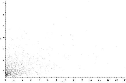
at the j-th step of the algorithm, ψt−1,j. As can be seen in Figure (1), they form a non

uniform random design in the xψ plane and are visibly more dense in the region next to

the axes, drawing in the xψ plane a ”falling star” pattern. So we need a method which is

capable to adapt the neighborhood of interest to the local density of predictors. Moreover,

the presence of a boundary in the domain (both the regression are nonnegative) should be

taken care of by the fact that the bias of the local linear estimator does not depend on the

marginal density of the predictors.

A practical rule for the choice of the span (that is, of the percentage of points of our

data included in the neighborhood of interest) is needed. As an efficient and fast method

to compute estimates of the MSE of our estimator we follow Hastie and Tibshirani (1990)

and use generalized cross validation (GCV). It can be proved that minimizing GCV is

asymptotically equivalent to minimize the mean square error. It each loop (and in the

final averaged smoothing), we therefore use the span that minimizes the quantity

GCV = n−

P

(xt−ψˆt,j)2

(n−trL)2 , (5)

where nis the sample size, ˆψt,j is the predictor ofxtcorresponding to the loopj and L

is the smoother matrix, that is the matrix that premultiplied to the predictors, yields the

estimates. The quantitytrLplays a role analogous to the number of degrees of freedom in

a standard linear regression.

Finally, it can be remarked from equation 3 that the regression has a conditionally

heteroskedastic error that calls for a weighted fit. Obviously, the true weights would

depend on the function we are estimating and are unknown. We therefore replace them

in each loop with the estimates of the conditional durations that were computed in the

3

Estimation of simulated processes

In this section we perform an assessment of the performance of the non parametric

speci-fication via a comparison with the estimates of a linear ACD model on different simulated

series. The first simulated series is characterized by an asymmetry in the conditional mean

equation, which has the following form:

f(xt−1, ψt−1) = 0.2 + 0.1xt−1+ (0.3I[xt

−160.5]+ 0.85

I_[xt

−1>0.5])ψt−1, (6)

and the conditional duration is Weibull distributed, with scale parameter such that its

mean is equal to one. The size of the generated sample is of 5000 observations. We

simulate 100 series from model (6). The simulated series are estimated by ML with a

linear ACD(1,1) specification and by the non parametric smoother described in Section

2.2 8 basic iterations and performing a final smooth based on the arithmetic mean of the

last K = 4 iterations. The performance of the parametric and non parametric estimators

are compared by computing two widely used measures of estimation errors. The first one

is the Mean Square Error (MSE), based on a quadratic loss function:

M SE= 1

nM M X l=1 n X i=1

( ˆψil−ψil)2, (7)

where i= 1, . . . , n= 5000 denotes thei−th estimated conditional mean within the series,

and l = 1, . . . , M = 100 labels the 100 series simulated from (6).

The second measure is the Mean Absolute Error (MAE):

M AE = 1

nM M X l=1 n X i=1

|ψˆil−ψil|. (8)

model, with no asymmetric component in the specification of the conditional mean

equa-tion. The functional form is of the conditional mean is

f(xt−1, ψt−1) = 0.1 + 0.1xt−1+ 0.75ψt−1, (9)

and the conditional distribution and the sample size are the same as in the first group

of simulated series. The settings of the parametric and non parametric estimators do not

change from the first example. In particular, we estimate a parametric ACD(1,1) model

which this time is correctly specified.

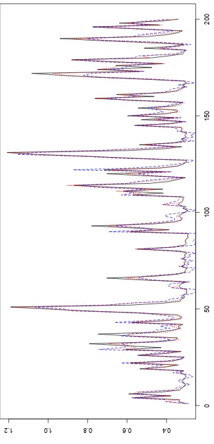
Figure 2 displays in a 200 data window an example of the evolution of the simulated

ψ (hence the true dgp), and of the ones estimated parametrically and non parametrically.

We can remark that the parametric estimator seems to overreact, and make big mistakes in

a small number of points. This characteristic had already been captured by the difference

between the MSE and TMSE of the parametric estimator.

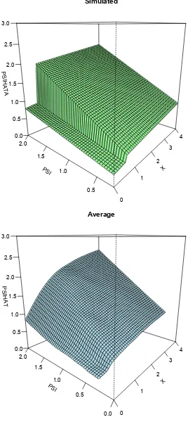
Figure 3 shows the surfaces generated from the nonlinear model in equation 6f(xt−1, ψt−1)

in their simulated version and in the one estimated non parametrically. The abrupt change

in the slope of f = ˆψt(xt−1, ψt−1) as a function of ψt−1 for x ≤ 0.5 and x > 0.5 is quite

visible in the bottom part of the estimated surface (near the origin), where data are very

dense and the bandwidth is rather small. Farther from the origin, observations in the

support become more sparse and the result is somewhat more smoothed. In any case, it

is clear that the slope increases as x increases. To complete the analysis on this group

of simulations, we give in table 1 an example of how the span minimizing the generalized

cross validation criterion evolves with the steps of the algorithm. It is rather visible that

the main loop converges quite early to a stable value.

both indices show that the the non parametric estimator overperforms the parametric one.

Both MSE and MAE decrease at each loop and further drop after the final averaging.

When instead the series is simulated starting from the linear ACD model, the parametric

estimator is correctly specified and, unsurprisingly, obtains the lowest MSE and MAE.

The non parametric estimator though seems quite able to select a large span and its errors

remain in the same order of magnitude. We don’t show the charts of the reconstructed

surfaces in this case as they appear to be rather uninformative flat planes.

4

Estimation of a financial data set

In this section, the non parametric specification of the ACD model is tested on a set of

financial data. The estimated series consists in a set of volume and price durations of

the following stocks traded in 1997 in the New York Stock Exchange: Boeing, Disney and

IBM. Trade, price and volume durations are considered.

4.1

Evidence on deseasonalized data

As noticed already in the seminal paper by Engle and Russell (1998), strong intraday

seasonality is present in tick-by-tick data, as durations have a tendency to be shorter on

average at the beginning and closing of trading sessions. It is therefore common to remove

seasonality by means of a non parametric regression (spline, Nadaraya-Watson, Fourier

series...) of raw durations on the time of the day and to fit data by ACD models once

they are deseasonalized. In this round of estimations, durations are adjusted by dividing

them by the estimated daily cyclical component computed by averaging the variable over

thirty minute intervals for each day in our sample. This is equivalent to assuming that

the trading day is divided in thirteen 30 minute bins (from 9h30 to 16h), and that each

practice, as each variable changes throughout the trading day. Assuming that such changes

happen gradually, cubic splines are then used on the thirty minute intervals to smooth the

time-of-day functions.

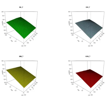
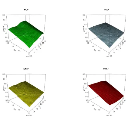
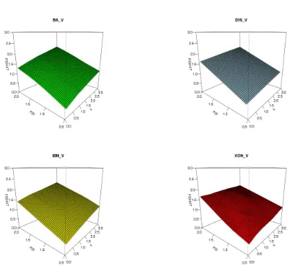
Figures 4, 5 and 6 present the surfaces estimated non parametrically with 10 loops and

a final average of the last 4.

The visual analysis suggests us some conclusions. First, some nonlinearity is present in

almost all surfaces, though it never reaches the extreme features of the discontinuity in data

simulated in the previous section. Second, some datasets, notably Disney volume but, to

lesser degree, Boing price and IBM trade durations, the surface is almost linear. This is also

supported by the very high values of the spans minimizing the generalized cross validation

(0.999, 0.995 and 0.981 respectively). In other datasets, the nonlinearities appear more

marked. Third, in these cases, the real data generating process in the conditional mean

equation seems to put a low weight on the lagged observation Xt−1, and the dependence

of ψt on ψt−1 appear to diminish with growing X. This is a reasonable feature. Let

us think about a regime switching model, dependent on whether the market speeds up

or slows down. When the market speeds up (short durations), we are more likely to

observe bunching in the data, that is, there is a bigger autocorrelation component in the

conditional mean equation, and so a stronger dependence of ψt onψt−1. When the market

cools down, we observe less clustering in the duration data, and the conditional duration

in the conditional mean is weaker.

We now proceed to compare the forecasting performances of the non parametric and

parametric estimators. We split the sample in two parts: the first 90% of the observations

are used for estimation, the 10%, for evaluation. Using the result of the estimation on the

first part of the sample, we use the conditional duration for time t estimated both

in table 4, along with the percentage gains obtained by non parametric estimation. We

also test for the significance of differences in forecast accuracy by performing a Diebold

and Mariano (1995) with respectively an asolute loss function for MAE and a squared one

fore MSE. In the table, percentage gains between parentheses are not significant at a 5%

level.

The non parametric estimator seems to yield an improvement in one-step-ahead forecast

accuracy in almost all cases, though only a few of them appear to be significant. Only

in the case of Disney volume durations the parametric ACD model has smaller, but not

significantly, forecast errors.

4.2

Empirical application: evaluation of the shocks impact curve

Engle and Russell (1998) noticed that the ACD model had the tendency to overpredict

after very long or very short durations. This would make a model with a concave shocks

impact function (the ACD one is linear) better suited as a forecasting tool. The desirability

for this feature was explicitely acknowledged in the subsequent literature and the Box-Cox

transformation-based ACD family of specifications proposed by Fernandes and Grammig

(2006) indeed show concavity in the shape of the curve. The model proposed in this paper

has not an a-priori form for the shock impact curve given that, depending on the resulted

estimated surface, the the response of the expected conditional duration to a shock in the

baseline duration can vary. As an experiment, we estimate our model with the same data

(quote durations for the IBM stock) used in Fernandes and Grammig (2006) and compute

the resulting shocks impact curve by fixing ψi−1 at 1 and letting ǫt−1 vary in order to

evaluate its impact on the value of the expected conditional duration ψi.

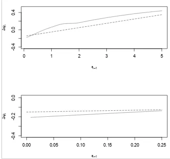
Figure 7 displays the curve resulting from the non parametric estimation along with the

one resulting from the estimation of a parametric ACD model. The result seems to confirm

benefit from its better flexibility and to produce a slightly concave response curve. It can

be noticed too that the concavity resulting from our estimator seems less pronounced than

the one observed in the estimations of the modes proposed by Fernandes and Grammig

(2006), this at least on the basis of a simple visual evaluation.

4.3

Inclusion of the time of the day as a covariate

The maximum likelihood estimation of linear ACD models on deseasonalized data can

be seen as a de facto semiparametric two-step procedure, where a first non parametric

deseasonalization is followed by the fully parametric estimation of the ACD model proper.

The literature offers some exceptions to this practice: Rodr´ıguez-Poo, Veredas, and Espasa

(2008), Brownlees and Gallo (2011) and Bortoluzzo, Morettin, and Toloi (2010). Yet,

this standard practice does not take into account a possible time-dependence of the ACD

parameters. The risk of this approach could be of missing some of the information contained

in the data and therefore providing suboptimal fit and forecasts if the object of analysis

are the original seasonality-affected observations.

In this subsection we exploit the flexibility of the non parametric ACD estimator and

include in the formula for the conditional duration the time of the day as an explanatory

variable. In this setup, equation 3 becomes

Dt=f(Dt−1, ψt−1, τt) +ηt, (10)

with

ηt =f(Dt−1, ψt−1, τt)(ǫt−1),

does not require major changes in the recursive procedure asτt is fully observable and can

be treated as an exogenous covariate. The practical implementation too is easily achieved

as the LOESS function in R accomodates a set of three explanatory variables instead of the

two used with deseasonalized data. In order to make forecasts comparable, we multiplied

parametric ACD one-step-ahead predictions with the same values of the estimated diurnal

effect used to deseasonalize the raw data before estimation.

Table 5 reports a comparison between forecast absolute and quadratic errors of

para-metric and non parapara-metric estimators. Like in the case of deseasonalized data, many

forecasting accuracies differences do not seem significant at the 5% level for price and

vol-ume durations. The joint estimation of seasonality seems instead to yield better forecasts

in the case of trade durations, possibly due to the larger sample size of these data sets

suggesting the presence of curse-of-dimensionality effect that penalizes the results for short

data series.

A visual account of the evolution of the non parametrically estimated surface is

pro-vided by figure 8, which displays contour plots of the estimated surface of Boing volume

durations computed at 30 minutes intervals from 9:30 am to 16 pm. The shape of the

estimated conditional duration is clearly varying during the day. Moreover contour lines

seemingly tend to shift gradually from one time period to the following one, suggesting a

clear pattern of time dependency of the parameters of the model. Analogous time patterns

of the estimated surface are present for all other durations of all stocks. This evidence

clearly suggests that the standard practice of separating the estimations of the seasonality

component and the conditional duration function risks to miss the opportunity of

exploit-ing significant information present in the data. Even in fully parametric specification it

may be therefore beneficial to include some form of interaction between time of the day

5

Conclusion

The non parametric specification of the ACD model encompasses most of the parametric

forms so far introduced to study high frequency transaction data, the only exception being

constituted by the models with two stochastic components, such as the SCD. The model can

be easily estimated by standard non parametric techniques, though a recursive approach

is necessary to deal with the fact that some regressors are not directly observable. The

simulated examples show that in the presence of asymmetry in the specification of the

conditional mean equation the non parametric estimator easily outperforms the symmetric

parametric one. An estimation of a financial data set does show a marginally better

performance of the non parametric model in terms of forecasting power. When diurnal

seasonality is included in the model and jointly estimated with the conditional duration

surface, the forecast accuracy gain of the non parametric estimator improves for some

stocks. Still, though not providing a specification test for parametric models, the non

parametric analysis can be useful as a benchmark in the choice of the right parametric

specification. The graphical study of the dependence of the conditional mean on its lags

that we carried out can give valuable information on the kind of parametric specification to

choose. Also comparing the predicting performances of the non parametric and parametric

estimators can help evaluating ex post the choice of the parametric specification.

A final word can be spent for what could be a further use of this estimation strategy

in empirical analysis. Though the advantages of using a consistent estimator that is

en-compassing most of the specifications currently used would allow for several applications,

we think that it could be beneficial to include in the regression of market microstructure

variable, such as volume, prices, bid-ask spread or, if available dummies about the arrival

the subject of a non parametric or eventually, a semiparametric analysis. We leave this

development for further research.

References

Bauwens, L., and P. Giot(2000): “The logarithmic ACD model: an application to the

bid-ask quote process of three NYSE stocks,”Annales d’Economie et de Statistique, 60,

Special Issue, ”Financial Market Microstructure”, 117–149.

(2003): “Asymmetric ACD models: introducing price information in ACD models

with a two state transition model,”Empirical Economics, 28(4), 709–731.

Bauwens, L., J. Grammig, P. Giot, and D. Veredas (2004): “A comparison of

financial duration models with density forecasts,” International Journal of Forecasting,

20, 589–609.

Bauwens, L., and D. Veredas (2004): “The stochastic conditional duration model:

a latent factor model for the analysis of financial durations,”Journal of Econometrics,

119(2), 381–412.

Bortoluzzo, A. B., P. A. Morettin, and C. M. Toloi (2010): “Time-varying

autoregressive conditional duration model,” Journal of Applied Statistics, 37(5), 847–

864.

Brownlees, C. T., F. Cipollini, and G. M. Gallo (2012): “Multiplicative error

models,”Handbook of Volatility Models and Their Applications. New Jersey: Wiley.

Brownlees, C. T., and G. M. Gallo(2011): “Shrinkage estimation of semiparametric

B¨uhlmann, P., and A. J. McNeil (2002): “An algorithm for nonparametric GARCH

modelling,” Computational Statistics and Data Analysis, 40, 665–683.

Cleveland, W.(1979): “Robust locally weighted regresson and smoothing scatterplots,”

Journal of the American Statistical Association, 74(368), 829–836.

De Luca, G., and P. Zuccolotto (2006): “Regime-switching Pareto distributions for

ACD models,”Computational Statistics & Data Analysis, 51(4), 2179–2191.

Diebold, F. X., and R. S. Mariano(2002): “Comparing predictive accuracy,”Journal

of Business & economic statistics, 20(1).

Engle, R., and G. Gonzalez-Rivera(1991): “Semiparametric ARCH Models,”

Jour-nal of Business and Economic Statistics, 9, 345–360.

Engle, R., and J. R. Russell (1998): “Autoregressive conditional duration: a new

approach for irregularly spaced transaction data,”Econometrica, 66, 1127–1162.

Fernandes, M., and J. Grammig (2006): “A family of autoregressive conditional

du-ration models,”Journal of Econometrics, 130(1), 1–23.

Franke, J., W. Hardle,andJ. Kreiss(2004): “Non parametric estimatio in a

stochas-tic volatility model,” Recent advances and trends in Nonparametric Statistics.

Franke, J. H., and M. Muller (2002): “Nonparametric estimation of GARCH

pro-cesses,”Applied Quantitative Finance, pp. 367–383.

Gerhard, F.,andN. Hautsch(2007): “A dynamic semiparametric proportional hazard

Hastie, T.,and R. Tibshirani(1990): Generalized additive models. Chapman and Hall.

Hautsch, N. (2011): Econometrics of financial high-frequency data. Springer.

Luca, G. D., and G. M. Gallo (2008): “Time-varying mixing weights in mixture

autoregressive conditional duration models,” Econometric Reviews, 28(1-3), 102–120.

Pacurar, M. (2008): “Autoregressive conditional duration (ACD) models in finance: A

survey of the theoretical and empirical literature,”Journal of Economic Surveys, 22(4),

711–751.

Rodr´ıguez-Poo, J. M., D. Veredas, and A. Espasa (2008): “Semiparametric

esti-mation for financial durations,” in High frequency financial econometrics, pp. 225–251.

Springer.

Wongsaart, P., J. Gao, and D. E. Allen (2010): “An alternative semiparametric

regression approach to nonlinear duration modeling: theory and application,” in

Nonlinear Linear

Loop

1 0.831 0.999

2 0.206 0.999

3 0.708 0.999

4 0.597 0.999

5 0.612 0.999

6 0.736 0.999

7 0.612 0.999

8 0.623 0.999

9 0.622 0.999

10 0.622 0.999

Average 0.621 0.999

Table 1: Evolution of the GCV-selected bandwidth in an estimation of a series of 5000 simulated nonlinear and linear ACD observations.

Nonlinear Linear

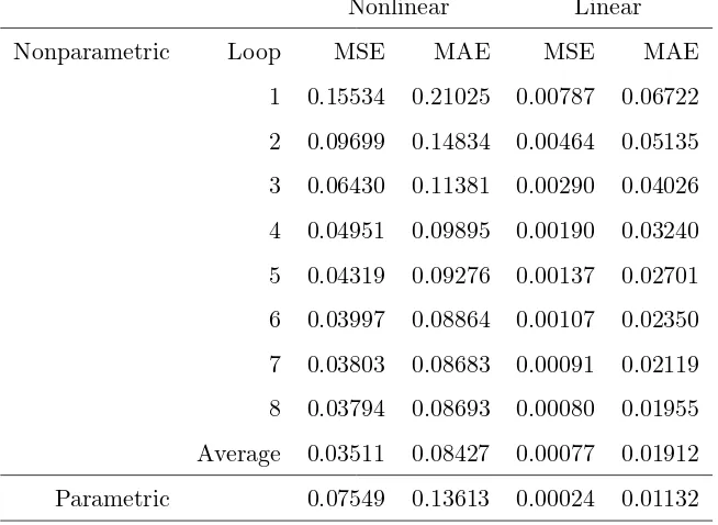
Nonparametric Loop MSE MAE MSE MAE

1 0.15534 0.21025 0.00787 0.06722

2 0.09699 0.14834 0.00464 0.05135

3 0.06430 0.11381 0.00290 0.04026

4 0.04951 0.09895 0.00190 0.03240

5 0.04319 0.09276 0.00137 0.02701

6 0.03997 0.08864 0.00107 0.02350

7 0.03803 0.08683 0.00091 0.02119

8 0.03794 0.08693 0.00080 0.01955

Average 0.03511 0.08427 0.00077 0.01912

1000 obs 5000 obs 10000 obs

Nonlinear Linear Nonlinear Linear Nonlinear Linear

Loop MSE MAE MSE MAE MSE MAE MSE MAE MSE MAE MSE MAE

1 0.060 0.120 0.0025 0.033 0.044 0.099 0.00054 0.015 0.042 0.098 0.00036 0.013

2 0.058 0.115 0.0028 0.036 0.037 0.088 0.00063 0.016 0.034 0.084 0.00039 0.013

3 0.057 0.114 0.0032 0.038 0.034 0.084 0.00072 0.017 0.030 0.078 0.00040 0.013

4 0.056 0.113 0.0036 0.040 0.032 0.082 0.00074 0.018 0.028 0.076 0.00042 0.014

5 0.056 0.113 0.0035 0.040 0.031 0.081 0.00074 0.017 0.027 0.074 0.00046 0.014

6 0.055 0.112 0.0035 0.040 0.031 0.081 0.00077 0.018 0.026 0.073 0.00045 0.014

7 0.057 0.113 0.0035 0.040 0.030 0.080 0.00078 0.018 0.026 0.073 0.00044 0.014

8 0.055 0.112 0.0036 0.040 0.030 0.080 0.00074 0.017 0.026 0.074 0.00044 0.014

9 0.056 0.113 0.0037 0.041 0.030 0.080 0.00077 0.018 0.026 0.073 0.00046 0.014

10 0.057 0.114 0.0038 0.040 0.030 0.080 0.00079 0.018 0.026 0.073 0.00049 0.014

avg 0.054 0.112 0.0033 0.038 0.030 0.080 0.00074 0.017 0.026 0.072 0.00045 0.014 par 0.086 0.143 0.0012 0.025 0.077 0.138 0.00024 0.011 0.074 0.135 0.00016 0.009

0 1 2 3 4 5 6 7 8 9 10 11 12 13 14 1

2 3 4 5 6 7

!

x

0

50

100

150

200

0.4

0.6

0.8 1.0

1.2

MSE MAE

Type Obs Stock Par Nonpar % Par Nonpar %

Trade 75435 Boeing 1.417 1.416 (0.02) 0.772 0.768 0.41

61630 Disney 1.426 1.425 (0.06) 0.818 0.816 (0.10)

136020 Ibm 1.240 1.240 (0.02) 0.742 0.741 0.17

74170 Exxon 1.275 1.274 (0.08) 0.771 0.771 (0.02)

Price 8682 Boeing 1.750 1.738 (0.58) 0.821 0.806 1.86

5985 Disney 1.362 1.360 (0.11) 0.765 0.761 (0.50)

18878 Ibm 1.305 1.301 (0.21) 0.754 0.749 (0.59)

12974 Exxon 2.243 2.107 6.44 0.849 0.831 2.04

Volume 4261 Boeing 0.415 0.409 1.31 0.483 0.478 1.01

3450 Disney 0.355 0.356 (-0.42) 0.465 0.465 (-0.09)

9684 Ibm 0.413 0.379 (0.18) 0.457 0.457 (0.46)

5597 Exxon 0.413 0.412 (0.29) 0.488 0.485 (0.56)

0 _{1 2} 3 ₄ 5

-0.4

0.0

0.4

!_i!1

!

!i

0.00 0.05 0.10 0.15 0.20 0.25

-0.4

-0.2

0.0

!_i!1

!

!i

Stats MSE MAE

Type Obs Mean Stdev Stock Par Nonpar % Par Nonpar %

trade 75435 32 42 Boeing 1584 1581 (0.22) 25 25 0.33

61630 39 50 Disney 2351 2351 (0.01) 32 32 (0.12)

136020 18 22 Ibm 438 437 0.22 13 13 0.42

74170 33 40 Exxon 1487 1485 0.17 25 23 (0.06)

price 8682 274 434 Boeing 160962 163029 (-1.28) 226 224 (0.82)

5985 396 555 Disney 273336 263796 3.49 309 308 0.44

18878 127 172 Ibm 24133 25915 0.83 98 97 0.74

12974 184 307 Exxon 85822 86463 (-0.75) 158 161 (-1.68)

volume 4261 560 463 Boeing 147635 150132 (-1.69) 275 275 (-0.22)

3450 690 499 Disney 190170 192158 (-1.04) 325 324 (0.30)

9684 249 207 Ibm 28009 27879 (0.46) 116 115 (0.66)

5597 428 343 Exxon 86696 87806 (-1.28) 212 211 (0.34)

hour 9.5 hour 10 hour 10.5

hour 11 hour 11.5 hour 12

hour 12.5 hour 13 hour 13.5

hour 14 hour 14.5 hour 15

hour 15.5 hour 16