New Highly Accurate Iterative Method of Third Order
Convergence for Finding The Multiple Roots of Nonlinear
Equations
N. A. A. Jamaludin1, N. M. A. Nik Long ∗1,2, and F. Ismail 1,2
1Department of Mathematics, Faculty of Science, Universiti Putra Malaysia, 43400 Serdang, Selangor, Malaysia
2Institute for Mathematical Research, Universiti Putra Malaysia, 43400 Serdang, Selangor, Malaysia
∗Corresponding author:[email protected]
We present a new third order convergence iterative method for mmultiple roots of nonlinear equation. The proposed method requires one evaluation of function and two evaluations of the first derivative of function. In numerical tests exhibit that the present method provides provides high accuracy numerical result as compared to other methods. The stability of the dynamical behaviour of iterative method is investigated by displaying the basin of attraction. Basin of attraction displays less black points which give us wider choices of initial guess in computation. Keywords: Basin of attraction, Multi-point iterative methods, Multiple roots, Nonlinear equations, Order of convergence.
I.
Introduction
Solving nonlinear equation accurately is one of the most important task in numerical analysis. The well-known Newton’s method for finding multiple roots,x∗ is written as
xk+1=xk−m
f(xk)
f0(xk)
. (1)
where m is multiplicity of roots. This method was developed by Schr¨oder and Stewart (1998), which converges quadratically. In recent years, some modification of Newton’s method for multiple roots with third order convergence have been developed and analyzed. Examples are Dong (1982), Dong (1987), Ferrara et al. (2015), Heydari et al. (2010), Homeier (2009), Sharifi et al. (2015) and Victory Jr and Neta (1983). All of those methods require the mul-tiplicity, m, to be known. Parida and Gupta (2008), Soleymani and Babajee (2013) and Yun (2009) developed the iterative methods with the unknown m. Chun et al. (2009), Hansen and Patrick (1976), Neta (2008) and Osada
(1994) developed the iterative methods which require the evaluation of second derivative of function.
In this paper we deal with the iterative meth-ods of third order convergence to find the mul-tiple roots x∗, of non-linear equation, with known multiplicity, m. Our proposed method is free from the evaluation of second derivative,
f00 of function.
II.
Construction of method
Osada (1994) proposed the third order one-point iterative method for finding the multiple roots of nonlinear equation,f(x) = 0 as
xk+1 =xk−
1
2m(m+ 1)
f(xk)
f0(x
k)
+1
2(m−1)
2f0(xk)
f00(x
k)
. (2)
multiple roots as
yk =xk−
2m m+ 2
f(xk)
f0(xk)
, (3)
where m is the multiplicity of multiple roots. With the help of Taylor’s series, we obtain
f00(xk)∼=
(m+ 2)f0(xk) [f0(xk)−f0(yk)]
2mf(xk)
. (4)
Substitute (4) into (2) and incorporate with (3), we have
yk =xk−
2m m+ 2
f(xk)
f0(x
k)
,
xk+1 =xk−
m(m+ 1)f(xk)
2f0(xk)
+ (m−1)
2mf(x
k)
(m+ 2) (f0(xk)−f0(yk))
.
(5)
The scheme in (5) is not in stable state as third order convergence. In order to archive the stable third order convergence, we write
yk= xk−
2m m+ 2
f(xk)
f0(xk)
,
xk+1 = xk−
m(m+ 1)f(xk)
αf0(x
k)
+ β(m−1)
2mf(x
k)
(m+ 2) (f0(x
k)−f0(yk))
,
(6)
where α and β are free disposable parameters. For simple root case, wherem= 1, method (6) becomes one point iterative Newton’s method, with the first step is void.
III.
Convergence Analysis
In this section, we describe a choice of param-eters α and β in order to get the third-order convergence for our scheme (6).
Theorem 1. Let x∗ ∈D be a multiple roots of a sufficiently smooth function f :D⊆R →R
defined on an open interval D with the multi-plicity m > 1, which includes x0 as an initial
approximation ofx∗. Then, the iterative meth-ods defined by (6) has third order convergence when
(
α = −−m2(m+2)2mm+mm(mm(+1)−4+m(m+2)),
β = m−m(m+2)1−m(4(mmm−(m1)+2)2 −m(m+2)m)2,
with the error term en+1 = 2(m
m−(q)m)c2 1e3n mqq−m3qm +
O(e4n).
Proof. Let en:=xn−x∗, en,y:=yn−x∗, ci:= m!
(m+i)!
fm+i(x∗)
fm(x∗) , c0 = 1, p=m+1, q=m+2, r= m−1. Using the fact that f(x∗) = 0, Taylor expansion of f atx∗ yields
f(xn) =emn 1 +c1en+c2e2n+c3e3n
+O(e4n) (7) and
f0(xn) =er(m+enpc1+e2n(q)c2
+e3n (m+ 3)c3+O(e4n)
). (8)
Thus
en,y =yn−x∗=
men
q +
2c1e2n
m(q)
+ −2(p)c
2
1+ 4mc2
e3n m2(q) +O(e
4
n). (9)
Forf(yn) we have
f(yn) =emn,y 1 +c1en,y+c2e2n,y+c3e3n,y
+O(e4n,y). (10)
Substituting (7)-(10) into (6) gives the error term as
en+1 =D1en+D2e2n+D3e3n+O(e4n),
where
D1 = 1−
1 2m
1 +m1
α +
2r2β mq−mmq2−m
! ,
(11)
D2 =
1 2m(−
p mα +
p2 m2α −
2r2β mq−mmq2−m
+2r
2qr m2p)qm+mm(4−mpq) β
m2(mmq−mqm)2 )c1,
(12)
D3 =
c21V + 2c2m(mmq−mqm)S
V =−m3mp2q4+m3pq3m(2 + 3m+m2
+ 2r2αβ)−mmq2m(3m2p2q2+ 4r2(−4
−2m+ 3m3+m4)αβ) +m2mqm(3mp2q3
+ 2r2(−16 +m(−8 +mp(4 +m)))αβ)
and
S =m2mpq3+m2q2m 2 + 3m+m2+ 2r2αβ
−2mmqm mpq2+r2(−4 +mq)αβ .
To obtain the third convergence order, it is nec-essary to choose Di= 0 (i= 1,2), which yield
α=− 2m
mp
−m2qm+mm(−4 +mq)
and
β =−m
−mqr(mmq−mqm)2
4r2 ,
and the error terms becomes
en+1 =
2 (mm−(q)m)c21e3n mqq−m3qm +O(e
4
n)
which completes the proof.
IV.
Numerical Analysis
Consider the following iterative methods of third order convergence
1. Chun et al.’s method (CBN) in (Chun et al., 2009) is given by
xk+1 =xk
−m (2γ−1)m+ 3−2γ
2
f(xk)
f0(x
k)
+γ(m−1)
2
2
f0(xk)
f00(x
k)
−m
2(1−γ)
2
f(xk)2f00(xk)
(f0(x
k))3
, (14)
whereγ =−1.
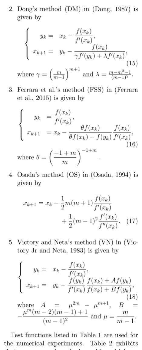
2. Dong’s method (DM) in (Dong, 1987) is given by
yk = xk−
f(xk)
f0(xk)
,
xk+1 = yk−
f(xk)
γf0(y
k) +λf0(xk)
,
(15) whereγ =mm−1m+1 and λ= m(m−m−1)2−21.
3. Ferrara et al.’s method (FSS) in (Ferrara et al., 2015) is given by
yk =
f(xk)
f0(x
k)
,
xk+1 =xk−
θf(xk)
θf(xk)−f(yk)
f(xk)
f0(xk)
,
(16)
whereθ=
−1 +m m
−1+m .
4. Osada’s method (OS) in (Osada, 1994) is given by
xk+1=xk−
1
2m(m+ 1)
f(xk)
f0(x
k)
+1
2(m−1)
2f0(xk)
f00(x
k)
. (17)
5. Victory and Neta’s method (VN) in (Vic-tory Jr and Neta, 1983) is given by
yk= xk−
f(xk)
f0(x
k)
,
xk+1 = yk−
f(yk)
f0(x
k)
f(xk) +Af(yk)
f(xk) +Bf(yk)
,
(18) where A = µ2m − µm+1, B =
−µ
m(m−2)(m−1) + 1
(m−1)2 and µ= m m−1.
and approximated computational order of con-vergence (ACOC) are defined, respectively, as (Grau-S´anchez et al., 2010)
COC ≈ ln|(xn+1−x
∗)/(x
n−x∗)|
ln|(xn−x∗)/(xn−1−x∗)|
(19)
and
ACOC≈ ln|(xn+1−xn)/(xn−xn−1)|
ln|(xn−xn−1)/(xn−1−xn−2)| .
(20)
V.
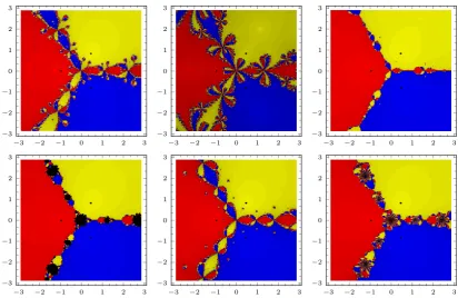
Basin of attraction
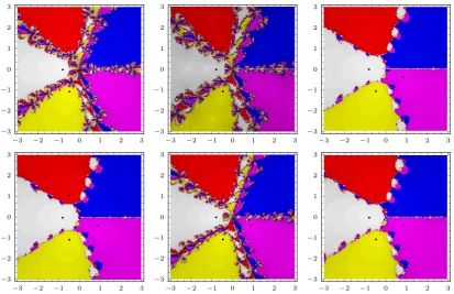
In this section we investigate the stability of the dynamical behaviour of iterative methods by utilizing the basin of attraction in complex plane. Let a square D ⊂ C and we choose the initial guess, z0 ∈ D. We assign the grid
300 ×300 point and set the square D with [−3.0,3.0]×[−3.0,3.0]. In basin of attraction we assign the different colour to different roots. The intensity of colour corresponding to the number of iteration needed to converge; region with the brighter colour require less number of iterations to converge to the roots, x∗ as com-pared to the darker colour. If the initial guess
x∗ is chosen in the black region, the numeri-cal convergence will not be archived even after 100 iterations with minimum tolerance>10−3. Table 3 shows the list of test functions with the complex roots used to generate basin of attrac-tion.
Figures 1-5 show the comparison of the dy-namical behaviour of the iterative methods listed in Table IV.. Its clearly seen that our newly developed iterative method provides less black points and larger brighter region as com-pared to others, which means the choice of ini-tial guess is vast.
Conclusion
We developed a new iterative method to obtain multiple roots of the nonlinear equation. The proposed method requires one evaluations of function and two evaluation of the first deriva-tive of function, and it is free from second derivative. Numerical performances exhibit that our method provides faster convergence and higher accuracy as compared to other methods with the same order of convergence. Basin of attraction displays that the proposed scheme contains less black points which gives us more choices of initial guess.
Acknowledgements
This project is supported by the Universiti Putra Malaysia under Putra Grant vot no: 9567900
References
[1] Changbum Chun, Hwa Ju Bae, and Beny Neta. New families of nonlinear third-order solvers for finding multiple roots.
Computers and Mathematics with Appli-cations, 57(9):1574–1582, 2009.
[2] C Dong. A basic theorem of constructing an iterative formula of the higher order for computing multiple roots of an equa-tion. Mathematics Numerical Sinica, 11: 445–450, 1982.
[3] Chen Dong. A family of multipoint iterative functions for finding multiple roots of equations. International Journal of Computer Mathematics, 21(3-4):363– 367, 1987.
[5] Miquel Grau-S´anchez, Miquel Noguera, and Jos´e Manuel Guti´errez. On some computational orders of convergence.
Applied Mathematics Letters, 23(4):472– 478, 2010.
[6] Eldon Hansen and Merrell Patrick. A family of root finding methods. Nu-merische Mathematik, 27(3):257–269, 1976.
[7] M Heydari, S M Hosseini, and G B Logh-mani. Convergence of a family of third-order methods free from second deriva-tives for finding multiple roots of nonlin-ear equations. World Applied Sciences Journal, 11(5):507–512, 2010.
[8] Herbert H H Homeier. On Newton-type methods for multiple roots with cu-bic convergence. Journal of Computa-tional and Applied Mathematics, 231(1): 249–254, 2009.
[9] B Neta. New third order nonlinear solvers for multiple roots. Applied Mathematics and Computations, 202(1):162–170, 2008.
[10] Naoki Osada. An optimal multiple root-finding method of order three. Jour-nal of ComputatioJour-nal and Applied Math-ematics, 51(1):131–133, 1994.
[11] P.K. Parida and D.K. Gupta. An improved method for finding mul-tiple roots and it’s multiplicity of nonlinear equations in r. Applied Mathematics and Computation, 202(2): 498 – 503, 2008. ISSN 0096-3003. doi: https://doi.org/10.1016/j.amc.2008.02.030.
URLhttp://www.sciencedirect.com/science/article/pii/S0096300308001240.
[12] E Schr¨oder and G W Stewart. On infinitely many algorithms for solving equations. Translation of paper by E. Schr¨oder, UMIACS-TR-92-121, 1998.
[13] S Sharifi, M Ferrara, N M A Nik Long, and M Salimi. Modified Potra-Pt´ak method to determine the multiple zeros
of nonlinear equations. arXiv preprint arXiv:1510.00319, 2015.
[14] F Soleymani and D K R Babajee. Com-puting multiple zeros using a class of quartically convergent methods. Alexan-dria Engineering Journal, 52(3):531–541, 2013.
[15] H D Victory Jr and B Neta. A higher order method for multiple zeros of non-linear functions. International Journal of Computer Mathematics, 12(3-4):329– 335, 1983.
[16] Beong In Yun. A derivative free it-erative method for finding multiple roots of nonlinear equations. Ap-plied Mathematics Letters, 22(12): 1859 – 1863, 2009. ISSN 0893-9659. doi: https://doi.org/10.1016/j.aml.2009.07.013.
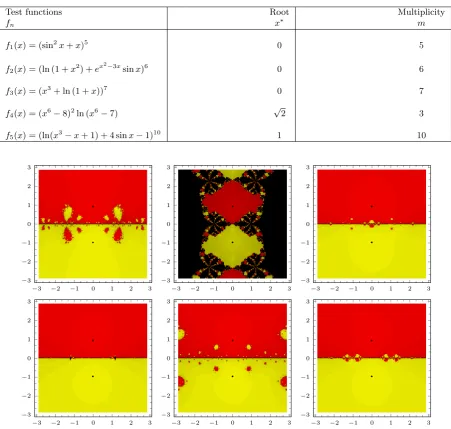
Table 1: List of Test Functions
Test functions Root Multiplicity
fn x∗ m
f1(x) = (sin2x+x)5 0 5
f2(x) = (ln (1 +x2) +ex 2−3x
sinx)6 0 6
f3(x) = (x3+ ln (1 +x))7 0 7
f4(x) = (x6−8)2ln (x6−7)
√
2 3
f5(x) = (ln(x3−x+ 1) + 4 sinx−1)10 1 10
−3 −2 −1 0 1 2 3 −3
−2 −1 0 1 2 3
−3 −2 −1 0 1 2 3 −3
−2 −1 0 1 2 3
−3 −2 −1 0 1 2 3 −3
−2 −1 0 1 2 3
−3 −2 −1 0 1 2 3 −3
−2 −1 0 1 2 3
−3 −2 −1 0 1 2 3 −3
−2 −1 0 1 2 3
−3 −2 −1 0 1 2 3 −3
−2 −1 0 1 2 3
Figure 1: Basin of attraction of Present Method, CBN, DM, FSS, OS, VN for test function
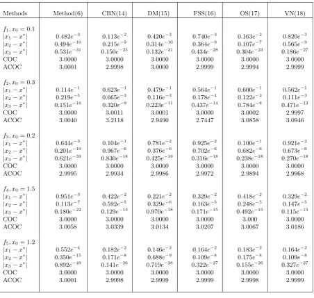
Table 2: Error, COC and ACOC of iterative methods
Methods Method(6) CBN(14) DM(15) FSS(16) OS(17) VN(18)
f1, x0= 0.1
|x1−x∗| 0.482e−3 0.113e−2 0.420e−3 0.740e−3 0.163e−2 0.820e−3 |x2−x∗| 0.494e−10 0.215e−8 0.314e−10 0.364e−9 0.107e−7 0.565e−9 |x3−x∗| 0.531e−31 0.150e−25 0.132e−31 0.434e−28 0.304e−23 0.186e−27
COC 3.0000 3.0000 3.0000 3.0000 3.0000 3.0000
ACOC 3.0001 2.9998 3.0000 2.9999 2.9994 2.9999
f2, x0= 0.3
|x1−x∗| 0.114e−1 0.623e−1 0.479e−1 0.564e−1 0.600e−1 0.562e−1 |x2−x∗| 0.219e−5 0.665e−3 0.116e−3 0.178e−4 0.122e−2 0.111e−3 |x3−x∗| 0.151e−16 0.320e−9 0.223e−11 0.437e−14 0.784e−8 0.471e−12
COC 3.0000 3.0011 3.0001 3.0000 3.0002 2.9997
ACOC 3.0040 3.2118 2.9490 2.7447 3.0858 3.0946
f3, x0= 0.2
|x1−x∗| 0.644e−3 0.104e−1 0.781e−2 0.925e−2 0.100e−1 0.921e−2 |x2−x∗| 0.201e−10 0.967e−6 0.376e−6 0.702e−6 0.682e−6 0.673e−6 |x3−x∗| 0.621e−33 0.830e−18 0.425e−19 0.316e−18 0.238e−18 0.270e−18
COC 3.0000 3.0000 3.0000 3.0000 3.0000 3.0000
ACOC 2.9995 2.9934 2.9986 2.9972 2.9894 2.9968
f4, x0= 1.5
|x1−x∗| 0.951e−3 0.422e−2 0.221e−2 0.329e−2 0.418e−2 0.329e−2 |x2−x∗| 0.113e−7 0.592e−5 0.329e−6 0.163e−5 0.248e−5 0.147e−5 |x3−x∗| 0.180e−22 0.129e−13 0.970e−18 0.171e−15 0.492e−15 0.115e−15
COC 3.0000 3.0000 3.0000 3.0000 3.000 3.0000
ACOC 3.0058 3.0339 3.0134 3.0207 3.0067 3.0186
f5, x0= 1.2
|x1−x∗| 0.552e−4 0.182e−2 0.146e−2 0.164e−2 0.183e−2 0.164e−2 |x2−x∗| 0.350e−15 0.171e−8 0.688e−9 0.109e−8 0.175e−8 0.109e−8 |x3−x∗| 0.892e−49 0.141e−26 0.719e−28 0.322e−27 0.155e−26 0.327e−27
COC 3.0000 3.0000 3.0000 3.0000 3.0000 3.0000
ACOC 3.0001 2.9998 2.9999 2.9999 2.9998 2.9999
Table 3: List of test functions and their roots
Test problem Root
pn(z) x∗
p1(z) = (z+1z)5 ±i
p2(z) = (z3−1)10 1, −0.5±0.866025i
p3(z) = (z3+ 1)3 −1, 0.5±0.866025i
p4(z) = (2z4−z)8 0, −0.39685±0.687365i, 0.793701
p5(z) = (z5−z2+ 1)15 −0.808731,
−3 −2 −1 0 1 2 3 −3
−2 −1 0 1 2 3
−3 −2 −1 0 1 2 3 −3
−2 −1 0 1 2 3
−3 −2 −1 0 1 2 3 −3
−2 −1 0 1 2 3
−3 −2 −1 0 1 2 3 −3
−2 −1 0 1 2 3
−3 −2 −1 0 1 2 3 −3
−2 −1 0 1 2 3
−3 −2 −1 0 1 2 3 −3
−2 −1 0 1 2 3
Figure 2: Basin of attraction of Present Method, CBN, DM, FSS, OS, VN for test function
p2(z).
−3 −2 −1 0 1 2 3 −3
−2 −1 0 1 2 3
−3 −2 −1 0 1 2 3 −3
−2 −1 0 1 2 3
−3 −2 −1 0 1 2 3 −3
−2 −1 0 1 2 3
−3 −2 −1 0 1 2 3 −3
−2 −1 0 1 2 3
−3 −2 −1 0 1 2 3 −3
−2 −1 0 1 2 3
−3 −2 −1 0 1 2 3 −3
−2 −1 0 1 2 3
Figure 3: Basin of attraction of Present Method, CBN, DM, FSS, OS, VN for test function
−3 −2 −1 0 1 2 3 −3
−2 −1 0 1 2 3
−3 −2 −1 0 1 2 3 −3
−2 −1 0 1 2 3
−3 −2 −1 0 1 2 3 −3
−2 −1 0 1 2 3
−3 −2 −1 0 1 2 3 −3
−2 −1 0 1 2 3
−3 −2 −1 0 1 2 3 −3
−2 −1 0 1 2 3
−3 −2 −1 0 1 2 3 −3
−2 −1 0 1 2 3
Figure 4: Basin of attraction of Present Method, CBN, DM, FSS, OS, VN for test function
p4(z).
−3 −2 −1 0 1 2 3 −3
−2 −1 0 1 2 3
−3 −2 −1 0 1 2 3 −3
−2 −1 0 1 2 3
−3 −2 −1 0 1 2 3 −3
−2 −1 0 1 2 3
−3 −2 −1 0 1 2 3 −3
−2 −1 0 1 2 3
−3 −2 −1 0 1 2 3 −3
−2 −1 0 1 2 3
−3 −2 −1 0 1 2 3 −3
−2 −1 0 1 2 3
Figure 5: Basin of attraction of Present Method, CBN, DM, FSS, OS, VN for test function