Search Space Properties for Learning a Class of Constraint based Grammars

Search Space Properties for Learning a Class of Constraint-based

Grammars

Smaranda Muresan

School of Communication and Information Rutgers University

4 Huntington St, New Brunswick, NJ, 08901

[email protected]

Abstract

We discuss a class of constraint-based grammars, Lexicalized Well-Founded Grammars (LWFGs) and present the theoretical underpinnings for learning these grammars from a representative set of positive examples. Given several assumptions, we define the search space as a complete grammar lattice. In order to prove a learnability theorem, we give a general algorithm through which the top and bottom elements of the complete grammar lattice can be built.

1 Introduction

There has been significant interest in grammar induction on the part of both formal languages and natural language processing communities. In this paper, we discuss the learnability of a re-cently introduced constraint-based grammar for-malism for deep linguistic processing, Lexical-ized Well-Founded Grammars (LWFGs) (san, 2006; Muresan and Rambow, 2007; Mure-san, 2011). Most formalisms used for deep lin-guistic processing, such as Tree Adjoining Gram-mars (Joshi and Schabes, 1997) and Head-driven Phrase Structure Grammar (HPSG) (Pollard and Sag, 1994) are not known to be accompanied by a formal guarantee of polynomial learnabil-ity. While stochastic grammar learning for sta-tistical parsing for some of these grammars has been achieved using large annotated treebanks (e.g., (Hockenmaier and Steedman, 2002; Clark and Curran, 2007; Shen, 2006)), LWFG is suited to learning in resource-poor settings. LWFG’s learning is a relational learning framework which characterizes the importance of substructures in the model not simply by frequency, as in most pre-vious work, but rather linguistically, by defining a

notion ofrepresentative examplesthat drives the acquisition process.

LWFGs can be seen as a type of Definite Clause Grammars (Pereira and Warren, 1980) where: 1) the Context-Free Grammar backbone is extended by introducing apartial ordering

re-lation among delexicalized nonterminals

(well-founded), 2) nonterminals are augmented with strings and their syntactic-semantic representa-tions; and 3) grammar rules have two types of constraints: one for semantic composition and one for ontology-based semantic interpretation (Muresan, 2006). In LWFG every stringwis as-sociated with a syntactic-semantic representation called semantic molecule h

b

. We call the tuple

(w, h_b)asyntagma:

(big table,0 B B B B B B @

h

2

6 4

cat np head X

nr sg

3

7 5

b

D

X1.isa = big,X.Y=X1,X.isa=table E

1

C C C C C C A )

The language generated by a LWFG consists of syntagmas, and not strings.

There are several properties and assumptions that are essential for LWFG learnability: 1) par-tial ordering relation on the delexicalized nonter-minal set (well-founded property); 2) each string has its linguistic category known (e.g.,npfor the phrase big table); 3) LWFGs are unambiguous; 4) LWFGs are non-terminally separable (Clark, 2006). Regarding unambiguity, we need to em-phasize that unambiguity is relative to a set of syntagmas (pairs of strings and their syntactic-semantic representations) and not to a set of natu-ral language strings. For example, the sentenceI

saw the man with a telescopeis ambiguous at the

string level (P P-attachment ambiguity), but it is unambiguous if we consider the syntagmas asso-ciated with it.

In this paper, for clarity of presentation, we make abstraction of the semantic representation and grammar constraints, and discuss the theo-retical underpinnings of Well-Founded Grammars (WFGs), which have all the properties of LWFGs that assures polynomial learnability. By defin-ing the operational and denotational semantics of WFGs, we are able to formally define the repre-sentative set of WFGs. Giving several assump-tions, we define the search space for WFG learn-ing as a complete grammar lattice by definlearn-ing the least upper bound and the greatest lower bound operators. The grammar lattice preserves the parsing of the representative set. We give a the-orem showing that this lattice is a complete gram-mar lattice. In order to give a learnability theorem, we give a general algorithm through which the top and the bottom elements of the complete grammar lattice can be built. The theoretical results ob-tained in this paper hold for the LWFG formalism. This theoretical result proves that the practical al-gorithms introduced by Muresan (2011) converge to the same target grammar.

2 Well-Founded Grammars

Well-Founded Grammars are a subclass of Context-Free Grammars where there is a partial ordering relation on the set of non-terminals. Definition 1. A Well-Founded Grammar (WFG)

is a 5-tuple,G=hΣ, NG,, P, Siwhere:

1. Σis a finite set of terminal symbols.

2. NG is a finite set of nonterminal symbols,

whereNG∩Σ =∅.

3. is a partial ordering relation on the set of

nonterminalsNG

4. Pis the set of grammar rules,P =PΣ∪PG,

PΣ∩PG=∅, where:

a) PΣ is the set of grammar rules whose

right-hand side are terminals, A → w,

where A _∈ NG and w ∈ Σ (empty string

cannot be derived). We denotepre(NG) ⊆

NG the set of pre-terminals, pre(NG) =

{A_|A_∈NG, w∈Σ, A→w∈PΣ}.

b) PG is the set of grammar rules A →

B1. . . Bn, where A ∈ (NG −pre(NG)),

Bi ∈ NG. For brevity, we denote a rule by

A _→ β, whereA _∈ (NG−pre(NG)), β ∈

N_G+. For every grammar ruleA→ β ∈PG

there is a direct relation between the

left-hand side nonterminalAand all the

nonter-minals on the right-hand sideBi ∈ β (i.e.,

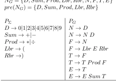
Σ =_{0,1,2,3,4,5,6,7,8,9,+,₋,_∗,_÷,(,)_} NG={D, Sum, P rod, Lbr, Rbr, N, F, T, E}

pre(NG) ={D, Sum, P rod, Lbr, Rbr}

PΣ PG

D→0|1|2|3|4|5|6|7|8|9 N →D

Sum→+|− N →N D

P rod_{→ ∗|÷} F _→N

Lbr_→( F _→Lbr E Rbr

Rbr_→) T _→F

T _→T P rod F E_→T

E_→E Sum T

Figure 1: A WFG for Mathematical Expressions

A Bi, or Bi A). If for all Bi ∈ β

we have that A Bi and A 6= Bi, the

grammar rule A _→ β is an ordered

non-recursive rule. Each nonterminal symbol

A _∈ (NG −pre(NG)) is a left-hand side

in at least one ordered non-recursive rule. In addition, the empty string cannot be derived from any nonterminal symbol and cycles are not allowed.

5. S _∈NGis the start nonterminal symbol, and

∀A_∈NG, S A(we use the same notation

for the reflexive, transitive closure of).

Besides the partial ordering relations , in WFGs the set of production rules P is split in PΣ andPG. For learning,PΣ is given, while the grammar rules inPGare learned.

In Figure 1 we give a WFG for Mathematical Expressions that will be used as a simple illus-trative example to present the formalism and the foundation of the search space for WFG learning. Every CFG G = _hΣ, NG, PΣ ∪ PG, Si can be efficiently tested to see whether it is a Well-Founded Grammar.

The derivation in WFGs is called ground

derivation and it can be seen as the bottom

up counterpart of the usual derivation. Given a WFG, G, the ground derivation relation, ∗⇒G, is defined as: A→w

A∗⇒Gw (A → w ∈ PΣ), and Bi∗⇒Gwi, i=1,...,n A→B1...Bn

A∗⇒Gw w=w1...wn

(w∈Σ+_).

The language of a grammarGis the set of all strings generated from the start symbol S, i.e., L(G) = {w|w ∈ Σ+, S ∗⇒G w}. The set of all

stringsgenerated bya grammarG isLw(G) =

notation, the set of strings generated bya

nonter-minal A of a grammar Gis Lw(A) = {w|w ∈

Σ+_{, A ∈ N}

G, A ∗⇒G w}, and the set of strings generated bya rule A _→ β of a grammar G is Lw(A → β) = {w|w ∈ Σ+,(A → β) ∗⇒G w}, where(A_→β)∗_⇒Gwdenotes the ground deriva-tionA∗_⇒Gwobtained using the ruleA_→βin the last derivation step. For a WFGG, we call a set of substringsEw ⊆Lw(G)a sublanguage ofG. Operational Semantics of WFGs. It has been shown that the operational semantics of a CFG corresponds to the language of the grammar (Wintner, 1999). Analogously, the operational se-mantics of a WFG,G, is the set of all strings gen-erated by the grammar,Lw(G).

Denotational Semantics of WFGs.As discussed in literature (Pereira and Shieber, 1984; Wint-ner, 1999), the denotational semantics of a gram-mar is defined through a fixpoint of a transforma-tional operator associated with the grammar. Let I _⊆Lw(G)be a subset of all strings generated by a grammarG. We define theimmediate derivation operator TG: 2Lw(G) → 2Lw(G), s.t.: TG(I) = {w∈Lw(G)|if(A→B1. . . Bn)∈PG ∧Bi ∗⇒G wi ∧ wi ∈ I then A ∗⇒G w}. If we denote TG ↑ 0 = ∅and TG ↑ (i+ 1) = TG(TG ↑ i), then we have that fori = 1, TG ↑ 1 = TG(∅) = {w ∈ Lw(G)|A ∈ pre(NG), A ∗⇒G w}.This cor-responds to the strings derived from preterminals, i.e.,w_∈ Σ. TGis analogous with the immediate consequence operator of definite logic programs (i.e., no negation) (van Emden and Kowalski, 1976; Denecker et al., 2001). TGis monotonous and hence the least fixpoint always exists (Tarski, 1955). This least fixpoint is unique, as for def-inite logic programs (van Emden and Kowalski, 1976). We have lf p(TG) = TG ↑ ω, where ω is the minimum limit ordinal. Thus, the denota-tional semantics of a grammar Gcan be seen as the least fixpoint of the immediate derivation op-erator. An assumption for learning WFGs is that the rules corresponding to grammar preterminals, A→w∈PΣ, are given, i.e.,TG(∅)is given.

As in the case of definite logic programs, the denotational semantics is equivalent with the op-erational one, i.e., Lw(G) = lf p(TG) . Based onTGwe can define theground derivation length

(gdl)for strings and theminimum ground

deriva-tion length (mgdl) for grammar rules, which are

key concepts in defining the representative setER of a WFG.

gdl(w) = min

w∈TG↑i (i)

mgdl(A_→β) = min

w∈Lw(A→β)

(gdl(w))

2.1 Properties and Principles for WFG Learning

In this section we present the main properties of WFGs, discussing their importance for learning. 1) Partial ordering relation (well-founded). In WFGs, the partial ordering relation on the nonterminal set NG allows the total ordering of grammar nonterminals and grammar rules, which allows the bottom-up learning of WFGs. WFG rules can be ordered or non-ordered, and they can be recursive or non-recursive. In addition, from the definition of WFGs, every non-terminal is a left-hand side in at least one ordered non-recursive rule, cycles are not allowed and the empty string cannot be derived, properties that guarantee the termination condition for learning. 2) Category Principle. Wintner (Wintner, 1999) calls observables for a grammarG all the deriv-able strings paired with the non-terminal that de-rives them: Ob(G) = _{hw, A_i|w _∈ Σ, A _∈ NG, A ∗⇒G w}, i.e., w ∈ Lw(A). We call w

a constituent and A its category. For example,

we can say that 1+1 is a constituent having the categoryexpression (E),1*1is a constituent hav-ing the category term (T), and 1 is a constituent having the categories digit(D), number (N),

fac-tor (F), term (T), expression (E). The Category

Principle for WFGs states thatthe observables are

known a-priori. When learning WFGs, the input

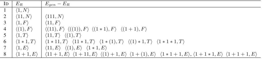
to the learner are observables hw, Ai. The cate-gory is used by the learner as the name of the left-hand side (lhs) nonterminal of the learned gram-mar rule. The Category Principle is met for natu-ral language, where observables (i.e., constituents and their linguistic categories) ca be identified: e.g.,hformal proposal, NPi,hvery loud, ADJPi. 3) Representative Set of a WFG (ER). Given an unambiguous1 _{Well-Founded Grammar G, a}

set of observables ER is called a representa-tive set ofG iff for each rule (A _→ β) _∈ PG there is a unique observable hw, Ai ∈ ER s.t.

1_{A WFGGis unambiguous if every string inL(G)has}

ID ER Egen−ER

1 h1, Ni

2 h11, N_{i h}111, N_i

3 h1, F_{i h}11, F_i

4 h(1), Fi h(11), Fi h((1)), Fi h(1∗1), Fi h(1 + 1), Fi

5 h1, T_{i h}11, T_{i h}(1), T_i

6 h1∗1, Ti h1∗11, Ti h11∗1, Ti h1∗(1), Ti h(1)∗1, Ti h1∗1∗1, Ti

7 h1, E_{i h}11, E_{i h}(1), E_{i h}1_∗1, E_i

8 h1 + 1, Ei h11 + 1, Ei h1 + 11, Ei h(1) + 1, Ei h1 + (1), Ei h1∗1 + 1, Ei,h1 + 1∗1, Ei h1 + 1 + 1, Ei

Figure 2: Examples for Learning the WFG in Figure 1

gdl(w) = mgdl(A _→ β), where w _∈ Lw(G). The nonterminal A is the category of the string w. ER contains the most simple strings ground derived by the grammarGpaired with their cat-egories. From this definition it is straightforward to show that |E_R| = _|P_G|. The partial ordering relation on the nonterminal set induces a total or-der on the representative setERas well as on the set of grammar rulesPG.

For the WFG induction, the representative set ER will be used by the learner to generate hy-potheses (i.e., grammar rules). The category will give the name of the left-hand side nonterminals (lhs) of the learned grammar rules. An exam-ple of a representative set ERfor the mathemat-ical expressions grammar from Figure 1 is given in Figure 2. For generalization the learner will use a generalization set of observables Egen = {hw, A_i|A_∈NG∧A⇒∗Gw}, whereER⊆Egen. An example of a generalization setEgenfor learn-ing the WFG from Figure 1 is given in Figure 2. 4) Semantics of a WFG reduced to a general-ization setEgen. Given a WFG Gand a gener-alization set Egen (not necessarily of G) the set S(G) = {hw, Ai|hw, Ai ∈ Egen ∧ A ∗⇒G w} is called the semantics of Greduced to the gen-eralization set Egen. In other words, S(G) will contain all the pairshw, Ai in the generalization set whose stringswcan be ground-derived by the grammarG,w _∈Lw(G). Given a grammar rule rA ∈PG, we callS(rA) = {hw, Ai|lhs(rA)=A∧ hw, A_{i ∈}E_gen∧rA∗⇒Gw}the semantics ofrA re-duced toEgen. The cardinality ofSis used during learning as performance criterion.

5) ER-parsing-preserving. We present the

rule specialization step and the rule

general-ization step of unambiguous WFGs, such that

they are ER-parsing-preserving and are the in-verse of each other. The property ofER -parsing-preserving means that both the initial and the

spe-cialized/generalized rules ground-derive the same stringwof the observablehw, Ai ∈ER. Therule specialization step:

A→αBγ B→β A→αβγ

is ER-parsing-preserving, if there exists hw, A_{i ∈}ERandrg ⇒∗Gwandrs∗G

0

⇒ w, whererg =A →αBγ , rB=B →β,rs=A →αβγ and rg ∈ PG,rB ∈ PG∩PG0,r_s ∈ P_G0 . We write

rg rB

` rs.2 The rule generalization step, which is also ER-parsing-preserving, is defined as the inverse of the rule specialization step and denoted byrs

rB

a rg.

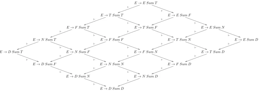
Since hw, Ai is an element of the representa-tive set,w is derived in the minimum number of derivation steps, and thus the rule rB is always an ordered, non-recursive rule. Examples ofER -parsing-preserving rule specialization steps are given in Figure 3, where all rules derive the same representative example1+1. In the derivation step E _→ N Sum D N→_`D E _→ D Sum D the ordered, non recursive rule rB = N → D is used. If the recursive rule N → N D were used, we would obtain a specialized rule E _→ N D Sum Dwhich does not preserve the pars-ing of the representative example1+1.

From both the specialization and the general-ization step we have thatLw(rg)⊇Lw(rs).

The goal of the rule specialization step is to ob-tain a new target grammarG0fromGby special-izing a rule ofG (G _{`</sub>r G0). Extending the no-tation to allow for the transitive closure of rule specialization, we have thatG <sub>`}∗ G0, and we say that the grammarG0isspecializedfrom the gram-mar G, using a finite number of rule specializa-tion steps that areER-parsing-preserving. Simi-larly, the goal of the rule generalization step is to

E→E Sum T `

uu

kkkkkkkkkk kkkkk

`SSSSSSSS₎₎ S S S S S S S

E→T Sum T `

uu

kkkkkkkkkk kkkkk

`SSSSSSSS)) S S S S S S

S E→E Sum F `

uu

kkkkkkkkkk kkkkk

`SSSSSSSS)) S S S S S S S

E→F Sum T `

uu

kkkkkkkkkk kkkkk

`SSSSSSSS)) S S S S S S

S E→T Sum F `

uu

kkkkkkkkkk kkkkk

`SSSSSSSS)) S S S S S S

S E→E Sum N `

uu

kkkkkkkkkk kkkkk

`SSSSSSSS)) S S S S S S S

E→N Sum T `

uu

kkkkkkkk kkkkkk

`SSSSSSSS)) S S S S S S

S E→F Sum F `

uu

kkkkkkkkkk kkkkk

`SSSSSSSS)) S S S S S S

S E→T Sum N `

uu

kkkkkkkkkk kkkkk

`SSSSSSSS)) S S S S S S

S E→E Sum D `

uu

kkkkkkkkkk kkkkk

E→D Sum T

`SSSSSSS₎₎ S S S S S S

S E→N Sum F `

uu

kkkkkkkkkk kkkkk

`SSSSSSSS₎₎ S S S S S S

S E→F Sum N `

uu

kkkkkkkkkk kkkkk

`SSSSSSSS₎₎ S S S S S S

S E→T Sum D `

uu

kkkkkkkkkk kkkkk

E→D Sum F

`SSSSSSSS)) S S S S S S

S E→N Sum N `

uu

kkkkkkkkkk kkkkk

`SSSSSSSS)) S S S S S S

S E→F Sum D `

uu

kkkkkkkkkk kkkkk

E→D Sum N

`SSSSSSSS)) S S S S S S

S E→N Sum D `

uu

kkkkkkkkkk kkkkk

E→D Sum D

Figure 3:ER-parsing preserving rule specialization steps for the grammar in Figure 1. obtain a new target grammarGfromG0 by

gen-eralizing a rule of G0. Extending the notation to allow for transitive closure of rule generalization, we have thatG0 _a∗ G, and we say that the grammar Gisgeneralizedfrom the grammarG0using a fi-nite number of rule generalization steps that are

ER-parsing-preserving. That is, ER is a

repre-sentative set for bothGandG0. TheER -parsing-preserving property allows us to define a class of grammars that form a complete grammar lattice used as search space for WFGs induction, as de-tailed in the next section.

6) Conformal Property. A WFG G is called

normalized w.r.t. a generalization set Egen, if

none of the grammar rules rs of G can be fur-ther generalized to a rule rg by the rule general-ization step such that S(rs) ⊂ S(rg). A WFG Gisconformal w.r.t. a generalization setEgen iff ∀hw, A_{i ∈} Egen we have that w ∈ Lw(G), andGis unambiguous and normalized w.r.t.Egen and the rule specialization step guarantees that S(rg) ⊃S(rs)for all grammars specialized from G. This property allows learning only from posi-tive examples.

7) Chains. We define achainas a set of ordered unary branching rules: {Bk → Bk−1, . . . , B2 → B1, B1 → β} such that all these rules ground-derive the same string w ∈ Σ+ (i.e., Bk Bk−1· · · B1 andB0 = β, such thatBi ∗⇒G w for 0 _≤ i _≤ k, where Bi ∈ NG for 1 ≤ i ≤ k). For our grammar {E → T, T → F, F → N, N _→ D_} is a chain, all these rules ground-deriving the string1. Chains are used to general-ize grammar rules during WFG learning (Fig. 3).

All the above mentioned properties are used to define the search space of WFG learning as a

complete grammar lattice.

2.2 Grammar Lattice as Search Space In this section we formally define a grammar lat-ticeL =hL,withat will be the search space for WFG learning. We first define the set of lattice elementsL.

Let>be a WFG conformal to a generalization setEgenthat includes the representative setERof the grammar>(Egen ⊇ER). LetL = {G|>

∗

` G} be the set of grammars specialized from >. We call>the top element ofL, and⊥ the

bot-tom elementofL, if∀G ∈ L,> `∗ G∧G ` ⊥∗ .

The bottom element,⊥, is the grammar special-ized from>, such that the right-hand side of all grammar rules contains only preterminals. We haveS(_>) =EgenandS(⊥)⊇ER.

There is a partial ordering among the elements ofL(the subsumptionw), which we define below. Definition 2. If G, G0 _{∈ L}, we say thatG

sub-sumesG0,GwG0, iffG`∗ G0 (i.e.,G0 is

special-ized fromG, andGis generalized fromG0)

We have that forG, G0 _{∈ L}, if G _w G0 then S(G)_⊇S(G0). That means that the subsumption

relation is semantic based.

top side

boundary

A

side bottom

w rA⇒∗"w

rA∈P"

rhs(r% A), r%A∈PG

B1

B2 B3 B4

(a) Boundary

r∗"⇒w

G1

G1!G2

G1

G2

G2

G1"G2

r∈P"

w

(b)lubandglboperators

E

}} }}

}} }}

}}

A A A A A A A A A

A r>:E→E Sum T

G1gG2 rG1gG2:E→T Sum T

E

Sum

G1

T

rG1:E→D Sum T

T

G2

F

rG2:E→T Sum N

F

G1fG2 N

G2

rG1fG2:E→D Sum N

N

D

D

G1

1 + 1

(c) Example forlubandglb

Figure 4 In order for L = _hL,_wi to form a lattice, we must define two operators: theleast upper bound

(lub), g and the greatest lower bound (glb), f, such that for any two elementsG1, G2 ∈ L, the elementsG1gG2 ∈ L andG1 fG2 ∈ Lexist (Tarski, 1955).

We first introduce the concept of boundary. Let rA ∈P>be a rule in grammar>, andrA0 its spe-cialized rule in grammar G ( > w G) (see Fig-ure 4a). Letpt(rA ∗>⇒ w)be the parse tree corre-sponding to the ground-derivationrA ∗>⇒ w. We callboundary of a grammar G ∈ L relative to pt(rA ∗>⇒ w),3 the right-hand side of the corre-sponding ruler_A0 ∈ PG, rA0

∗G

⇒ w, i.e. bd(G) =

{B_|r_A0 _∈ PG ∧B ∈ rhs(rA0 )}4(see Figure 4a). For the example in Figure 4c, the rule in grammar >isE → E Sum T, the rule in grammarG1 is E _→ D Sum T. Thus,bd(G1) = {D, Sum, T} We define thebottom-sidebs(G)of a grammarG relative to the parse treept(rA ∗>⇒ w), as the for-est composed of all the subtrees in pt(rA ⇒∗> w) whose roots are on bd(G) (e.g., subtrees with

roots at B1, B2, B3, B4 in Figure 4a). For the example in Figure 4c,bs(G1)will be the forest of subtrees of the parse treept(r_>⇒∗>1 + 1)with the

rootsD, SumandT on the boundarybd(G1)of grammarG1. We define thetop-side ts(G)of a grammarGrelative to the parse treept(rA⇒∗>w), as the subtree in pt(rA ∗>⇒ w) rooted at A and

3_{All grammarsG∈ LareE}

R-parsing-preserving and all

boundaries ofGare in the parse trees of the ground deriva-tions of>grammar rules.

4_{The notation of bd(G), ts(G), bs(G) ignores the rule}

relative to which these concepts are defined, and in the re-mainder of this paper we implicitly understand that the rela-tions hold for all grammar rules.

whose leaf nodes are onbd(G)(e.g.,B1,B2,B3 andB4 in Figure 4a). For the example in Figure 4c, ts(G1) will be the subtree of the parse tree pt(r_> ∗>_⇒1 + 1)rooted atEand the leaf nodesD, SumandTon the boundarybd(G1)of the gram-marG1. We have thatts(G)∩bs(G) = bd(G), ts(G)_∪bs(G) =pt(rA∗>⇒w).

For any two elementsG1, G2 ∈ L, thelub ele-ment ofG1, G2 is the minimum element that has the boundary above the boundaries ofG1andG2. Theglb element ofG1, G2 is the maximum ele-ment that has the boundary below the boundaries ofG1andG2. Thus,lubandglbare defined such that for all grammar rules we have:

ts(G1gG2) =ts(G1)∩ts(G2)

bs(G1fG2) =bs(G1)∩bs(G2) (1)

as can be seen in Figure 4b, 4c.5_{In order to have a}

complete lattice, the property must hold∀G ⊆ L:

ts(gG∈GG) =

\

G∈G

ts(G)

bs(fG∈GG) =

\

G∈G

bs(G) (2)

Lemma 1. L = hL,wi together with the lub

and glb operators guarantees that for any two

grammars G1, G2 ∈ L the following property

holds:G1gG2 wG1, G2 wG1fG2

Theorem 1. L = _hL,_wi together with the lub

andglboperators forms a complete lattice.

Proof. Besides the property given in Lemma 1,

lub and glb operators are computed w.r.t. (2), such that we havets(gG∈LG) =TG∈Lts(G) =

5_{The intersection of two trees is the maximum common}

S(!) =Egen

S(G2)

S(G1)

ER S(⊥)

S(G1!G2)

S(G1"G2)

Figure 5: WFG semantics reduced toEgen

ts(_>), bs(fG∈LG) = TG∈Lbs(G) = bs(⊥),

which gives the uniqueness of > and ⊥ ele-ments.

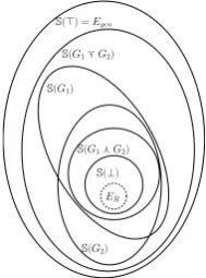
Similar to the subsumption relation w, the lub g andglb f operators are semantic-based. In the complete latticeL=_hL,_wi,_∀G1, G2 ∈ L we have:

S(G1gG2)⊇S(G1)∪S(G2).

S(G1fG2)⊆S(G1)∩S(G2)

(3)

Thus, the complete grammar lattice is semantic-based (Figure 5). It is straightforward to prove that L = hL,wi has all the known properties (i.e., idempotency, commutativity, associativity, absorption,>and⊥laws, distributivity).

2.3 Learnability Theorem

In oder to give a learnability theorem we need to show that⊥and>elements of the lattice can be built. Through Algorithm 1 we show that giving the set of examplesERandEgen, the⊥grammar can be built and the>grammar can be learned by generalizing the⊥grammar. The grammar gener-alization is determinate if the rule genergener-alization step is determinate. Before describing Algorithm 1 we introduce the concepts of determinate

gen-eralizableand give a lemma that states that given

a grammar>conformal withEgen, for any gram-marsGspecialized from>, all the grammar rules are determinate generalizable if all the chains of the>grammar are known.

Definition 3. A grammar rule r0_{A ∈} PG is

de-terminate generalizable if forβ ∈ rhs(r0_A)there

exists a unique rule rB = (B → β) such that

r_A0 raB rAwithS(r0A) ⊂S(rA). We use the

nota-tionr0_A 1_a⊂ rAfor the determinate generalization

step with semantic increase.

The only rule generalization steps allowed in the grammar induction process are those which guarantee the relationS(rs)⊂S(rg)that ensures that all the generalized grammars belong to the grammar lattice. This property allows the gram-mar induction based only on positive examples. We use the notationr0_ArB_a⊂rAfor the generaliza-tion step with semantic increase.

This step can be nondeterminate due to chain rules. Letch_> be a chain of rules in a WFG> conformal w.r.t a generalization setEgen,ch> =

{Bk → Bk−1, . . . , B2 → B1, B1 → β}. All the chain rules, but the last, are unary branching rules. The last rule is the minimal chain rule. For our example, ch_> = _{E _→ T, T _→ F, F _→ N, N → D}. For the ⊥ grammar of a lattice that has>as its top element, the aforementioned chain becomes ch_⊥ = _{Bk → β⊥, . . . , B2 → β_⊥, B1 → β⊥}, whereβ⊥ contains only

preter-minals and the rule order is unknown. By theER -parsing-preserving property of the rule specializa-tion step, the same string is ground-derived from thech_⊥ rules. Thus, the ⊥grammar is ambigu-ous. For our example, ch_⊥ = _{E _→ D, T _→ D, F _→D, N _→D_}.

We denote by ch = _{rk, . . . , r2, r1}, one or more chains in any lattice grammar, where the rule order is unknown. The minimal chain rules rm can always be determined if rm ∈ ch s.t. ∀r ∈ ch − {rm} ∧ rm

r

a rmg we have that S(rm) = S(rmg)(see alsoMinRulealgorithm). By the consequence of the conformal property, the generalization steprm

r

armgis not allowed, since it does not produce any increase in rule seman-tics. That is, a minimal chain rule cannot be gen-eralized by any other chain rule with an increase in its semantics. Given ch_⊥ and the aforemen-tioned property of the minimal chain rules we can recoverch_>byChains Recoveryalgorithm. Lemma 2. Given a WFG>conformal w.r.t a

gen-eralization setEgen, for any grammarGderived

from>all rules are determinate generalizable if

all chains of the grammar > (i.e., all ch_>) are

known (i.e., recovered by Chains Recovery

algorithm).

Proof. The only case of rule generalization step

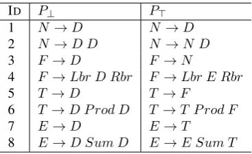
ID P⊥ P>

1 N _→D N _→D

2 N _→D D N _→N D

3 F _→D F _→N

4 F _→Lbr D Rbr F _→Lbr E Rbr

5 T _→D T _→F

6 T _→D P rod D T _→T P rod F

7 E_→D E_→T

8 E_→D Sum D E_→E Sum T

Figure 6: Examples ofP_⊥and learnedP_>

ch_⊥, whereBi → β⊥

Bj→β⊥⊂

a Bi → Bj holds for allBj ≺Bi. Thus, keeping (or recovering) the orderedch_> in any grammarG derived from_>, all the other grammar rules are determinate gen-eralizable.

We now introduce Algorithm 1, which given the representative set ER and the generalization setEgen, builds the⊥and>grammars. First, an assumption in our learning model is that the rules corresponding to the grammar preterminals (PΣ) are given. Thus, for a given representative setER, we can build the grammar⊥in the following way: for each observablehw, Ai ∈ERthe categoryA gives the name of the left-hand side nonterminal of the grammar rule, while the right-hand side is constructed using a bottom-up active chart parser (Kay, 1973) (line 1 in Algorithm 1). For our math-ematical expressions example, given ER in Fig-ure 2 andPΣ in Figure 1, the rules of the bottom grammarP_⊥are given in Figure 6.

Algorithm 1Top(ER, Egen) 1: P_⊥←Bottom(ER)

2: P_{> ←} Chains Recovery (P_⊥, ER, Egen) {P_>is determinate generalizable_}

3: while∃r_∈P>s.t. r

1⊂

a rgdo 4: r_←rg;

5: end while

6: returnP>

In order to build the > element (lines 2-5 in Algorithm 1), we first need to apply theChain recovery algorithm to the lattice ⊥ grammar (line 2 in Algorithm 1). Chains Recovery first detects all ch = ch_⊥ which contain rules with identical right-hand side (line 5-6). Then, allch_⊥rules are transformed inch_> by general-izing them through the minimal chain rule (lines 10-17). The generalization step r rma⊂ rg

guar-Algorithm 2Chains Recovery

1: Input:P_⊥, ER, Egen

2: Output:P_⊥which contains allch_>

3: whileER6=∅do

4: _hw, c_{i ←}f irst(ER)

5: ch← {r∈P⊥|r∗⊥⇒w} {ch=ch⊥}

6: lch← {lhs(r)|r∈ch}

7: for eachc_∈lchdo

8: ER←ER− {hw, ci}

9: end for

10: while|ch_|>1do

11: rm←MinRule(ch) 12: ch_←ch_{− {}rm} 13: lch_←lch_{− {}lhs(rm)}

14: for eachr_∈P_⊥∧lhs(r)_∈lch s.t. rrm_a⊂rg

do

15: r_←rg

16: end for

17: end while

18: end while

19: return:P⊥

Algorithm 3MinRule

1: Input:the chainch

2: for eachrm∈chdo

3: f ind←true

4: for eachr∈ch− {rm}do

5: if rm r

armg∧S(rm)⊂S(rmg)then 6: f ind_←f alse

7: end if

8: end for

9: iff ind==truethen

10: returnrm

11: end if

12: end for

antees the semantic increaseS(rg) ⊃S(r)for all the rulesrwhich are generalized throughrm, thus being the inverse of the rule specialization step in the grammar lattice. The rulesr are either chain rules or rules having the same left-hand side as the chain rules. The returned setP_⊥ contains all unary branching rules (ch_>) of the > grammar. The efficiency ofChain Recovery algorithm isO(_|E_{R| ∗ |}β_{| ∗ |}E_gen|). Therefore, in Algorithm

1 the setP_> initially contains determinate gener-alizable rules and the while loop (lines 3-5, Alg 1) can determinately generalize all the gram-mar rules. In Figure 6, the gramgram-marP_>is learned by Algorithm 1, based only on the examples in Figure 2 andPΣin Figure 1.

the representative set of a WFG G conformal

w.r.t a generalization set Egen ⊇ ER, then

Top(ER, Egen) algorithm computes the lattice>

element such thatS(_>) =Egen.

Proof. Since G is normalized, none of its

rule can be generalized with increase in se-mantics. Starting with the ⊥ element, after

Chains Recovery all rules that can be gen-eralized with semantic increase through the rule generalization step, are determinate generaliz-able. This means that the grammar generalization sequence⊥, G1, . . . , Gn,>, ensures the semantic increase ofS(Gi) so that the generalization pro-cess ends at the semantic limitS(_>) =Egen.

For WFGs which have rules that can be ei-ther left or right recursive, the top element is unique only if we impose a direction of gener-alization in the rule’s right-hand side (e.g., left to right). Another way to guarantee uniqueness of the top element is to add constraints at the grammar rules. In our example, if we augment de grammar nonterminals with expression val-ues (semantic interpretation) and we add con-straints at the grammar rules we have E(v) _→

E(v1) Sum(op) T(v2) : {v ← v1 op v2}. With the generalization exampleh5−3−1, E(1)i ∈ Egen we can generalize the ruleE → T Sum T only to E _→ E Sum T and not to E _→ T Sum E because 1 = (5−3)−1 and1 6= 5₋(3₋1). For our Lexicalized Well-Founded

Grammars this problem is solved by associating strings with their syntactic-semantic representa-tions and by having semantic compositional con-straints at the grammar rule level.

3 Conclusions

In this paper, we discussed the learnability of Lex-icalized Well-Founded Grammars. We introduced the class of well-founded grammars and presented the theoretical underpinnings for learning these grammars from a representative set of positive ex-amples. We proved that under several assump-tions the search space for learning these gram-mars is a complete grammar lattice. We presented a general algorithm which builds the top and the bottom elements of the complete grammar lattice and gave a learnability theorem. The theoretical results obtained in this paper hold for the LWFG formalism, which is suitable for deep linguistic processing.

References

Stephen Clark and James R. Curran. 2007. Wide-coverage efficient statistical parsing with ccg and log-linear models. Computational Linguistics, 33(4).

Alexander Clark. 2006. PAC-learning unambiguous NTS languages. InProceedings of the 8th Interna-tional Colloquium on Grammatical Inference (ICGI 2006), pages 59–71.

Marc Denecker, Maurice Bruynooghe, and Victor W. Marek. 2001. Logic programming revisited: Logic programs as inductive definitions. ACM Transac-tions on Computational Logic, 2(4):623–654. Julia Hockenmaier and Mark Steedman. 2002.

Gen-erative models for statistical parsing with combina-tory categorial grammar. InProceedings of the ACL ’02, pages 335–342.

Aravind Joshi and Yves Schabes. 1997. Tree-Adjoining Grammars. In G. Rozenberg and A. Sa-lomaa, editors, Handbook of Formal Languages, volume 3, chapter 2, pages 69–124. Springer, Berlin,New York.

Martin Kay. 1973. The MIND system. In Randall Rustin, editor,Natural Language Processing, pages 155–188. Algorithmics Press, New York.

Smaranda Muresan and Owen Rambow. 2007. Gram-mar approximation by representative sublanguage: A new model for language learning. In Proceed-ings of ACL’07.

Smaranda Muresan. 2006. Learning Constraint-based Grammars from Representative Examples: Theory and Applications. Ph.D. thesis, Columbia University.

Smaranda Muresan. 2011. Learning for deep lan-guage understanding. InProceedings of IJCAI-11. Fernando C. Pereira and Stuart M. Shieber. 1984. The

semantics of grammar formalisms seen as computer languages. InProceeding of the ACL 1984. Fernando C. Pereira and David H.D Warren. 1980.

Definite Clause Grammars for language analysis.

Artificial Intelligence, 13:231–278.

Carl Pollard and Ivan Sag. 1994. Head-Driven Phrase Structure Grammar. University of Chicago Press, Chicago, Illinois.

Libin Shen. 2006. Statistical LTAG Parsing. Ph.D. thesis, University of Pennsylvania, Philadelphia, PA, USA. AAI3225543.

Alfred Tarski. 1955. Lattice-theoretic fixpoint theo-rem and its applications. Pacific Journal of Mathe-matics, 5(2):285–309.

Maarten H. van Emden and Robert A. Kowalski. 1976. The semantics of predicate logic as a programming language.Journal of the ACM, 23(4):733–742. Shuly Wintner. 1999. Compositional semantics