Abstract—The short term electric load forecasting which is generally from one hour to one week is one of the intelligent electric grid (smart grid), for control of stable load supply hour-to-hour or day-to-day. The difficulty of short time forecasting is that the trend of time series usually change, and the non-adaptive auto-regressive integrated moving average (ARIMA) could not fit accurately. To solve that problem, conventional adaptive ARIMA with constant forgetting factor that gives a larger weight to more recent train data for dealing with non-stationary change of stochastic disturbance. The forgetting factor governs the recursive least squares (RLS) algorithm. However, constant forgetting factor usually result in over-fitting that increases forecasting error. A new adaptive ARIMA is proposed in this paper to improve the accuracy with lazy learning algorithm to reduce over-fitting error.
Index Terms—Intelligent electric grid, RLS algorithm, forgetting factor, ARIMA, lazy learning algorithm.
I. INTRODUCTION
HE Electric power quality is the vital consideration of steady power supply in industry. The running well power quality could be defined as stable electric load with normal range that is determined by technical requirement.[1]
The intelligent electric grid could improve the efficiency and reduce rates of power supply anomalies and fluctuations. For smart grid, the system is established with a variety of infrastructure, electric equipment and intelligence system [2]. The intelligence layer in electric utility could establish a more responsive grid that balances the power supply and demand. In industry, technologies of intelligent grid includes analyzing data that is gathered from electric devices and integrating the intelligent operation systems. The purpose of intelligent system is to decrease the possibility rate of power outages, which could improve economic benefits, according to industry standard that excessive amplitude of power fluctuations could result in damage of electrical equipment.
Chengze LI. Waseda University Graduate School of Information Production and System (IPS), Japan. (e-mail: [email protected]).
Tomohiro MURATA, Professor of Waseda University Graduate School of Information Production and System (IPS), Japan. (e-mail: [email protected]).
The smart monitoring device could improve the robustness and reliability of distributive power grid. [3]
Prediction of electric load is one part of the construction of intelligent grid composited with intelligent electric devices and related intelligent software. It is possible to adjust the electric load in stable way by analyzing forecasting results, which is vital part of production of power generation and supply in smart grid. [4]
There are several related methods of short term electric load forecasting are commonly used in engineering, such as neural network, regression. The neural network is a non-parametric model and has advanced supervise learning ability but needs to be trained before applied [5]. Regression is a conventional method that it is able to determine the relative influence of one or more predictor variables to the criterion value. However, it is easy for regression to result in over-fitting or under-fitting.
In this paper, ARIMA model that is usually used in nonlinear time series is selected to be improved to get result that is more accurate. However, conventional non-adaptive ARIMA has a drawback of its static model that could not refresh fitness when the trend of time series have changed. That drawback results in decrease of the forecasting accuracy.
II. FORMULATION OF PROBLEM
A. Difficulties of short time period forecasting
Difficulties of short time period electricity load forecasting usually include two parts. First difficulty is non-stationary change of stochastic disturbance in short-term electricity demand. Second difficulty is non-stationary change of trend in short-term electricity demand. Forecasting method for short-term electricity demand should be robust and adaptive against non-stationary change.[6]
The non-adaptive ARIMA (p,d,q) is shown as following: Yt = (φ1Yt-1 +φ2Yt-2+...+φpYt-p)
d
+et +θ1et-1 + ...+θpet-q (1)Moreover, the coefficients of function are:
Ψ = (φ1, φ2, …, φp) (2) Θ = (θ1, θ2, …, θq) (3) Difference operator is:
d t
t
Y
Y
Y
d
t (4)B. CONVENTIONAL ADAPTIVE ARIMA MODEL
That above non-adaptive ARIMA (p,d,q) model need to be updated according to non-stationary change of time series data including sharp demand change in short period. To solve those problems, considering the adaptive ARIMA model to fit
Adaptive ARIMA Model based on Lazy
Learning Algorithm for Short Period Electric
Load Forecasting
Chengze LI, Tomohiro MURATA.
better. In addition, conventional adaptive ARIMA is based on RLS-forgetting factor algorithm, as one of the Kalman filters family, which is used to increase the weight of more recent train data. Because the performance of RLS algorithm in stability and tracking is based on forgetting factor, as mention above, constant forgetting factor has an unwanted performance of overfitting. Conventional Adaptive ARIMA of RLS-forgetting factor update parameters[7] in this following way. The error between forecasted data and actual data Yt:
]
)
[(
)
(
1 1 2 2 1 1 1 1 q t q t t d p t p t t n p t n q t te
e
e
Y
Y
Y
Y
t
L
(5) The weighted least squares error function C which is desire to minimize:2 1
)
(
)
(
L
t
C
n (6)2 1
)
(
)
(
L
t
C
n (7) λ is constant forgetting factor, λ
(
0
,
1
)
.Adaptation of forecasting function's coefficient Ψ and Θ to minimize C(ψ) and C(Θ), and the
*and Θ* are calculated as following:)
(
min
arg
*
C
(8))
(
min
arg
*
C
(9) However, the drawbacks of the conventional Adaptive ARIMA model is that the RLS-Forgetting factor algorithm by using constant λ is proposed but constant λ need to be decided by experiment and is not enough for Adaptation of ARIMA against overfitting problem[8]. For example, when λ is close to 1, which results in low misadjustment & good stability and tracking capabilities are reduced in the same time. When λ is smaller, it could improves tracking capabilities, but increases misadjustment. Therefore, we need variable weight parameter, and it is proposed by using recursive least square algorithm, and KNN-weight algorithm.III. PROPOSED METHOD
A. Observation time window
Lazy learning algorithm provides useful training algorithms based on local time series data. In this paper, KNN that is one of the lazy learning algorithms is used to select the train data for local learning could create observation time window.
The k-nearest neighbors (KNN) is a kind of lazy learning algorithm, which is usually used to applied into local learning. Generally, KNN is based on the Euclidean distance to calculate similarity between center points and other samples. However, this paper proposes a method to select the train data to establish the observation time window by using KNN’s idea.
The observation time window could choose k points nearest to the most recent data point xs, andxtis the t-th sample point
nearest to xs. In the observation time window, measuring the
Euclidean distance between xt and xs, and that is related to
Gaussian RBF for giving larger weight to more recent data. The observation time window is used for solving the problem of overfitting and underfitting.
B.Update of parameters
The RLS algorithm is used for the update of ARIMA model’s parameters to make adaptive prediction. It is noteworthy that parameter update could avoid overfitting caused by the not good global learning.[9]
Additionally, the idea of lazing learning algorithm, which is do local learning, could solve the problem of overfitting with a novel selection method of train data and determination of adaptive weights that has better performance than constant forgetting factor. [10]
Proposed adaptation method of weight and (p, d, q) parameters based on lazy learning algorithm is delivered to improve the prediction performance. Every time a point is predicted, the parameter is updated once. The proposed parameters update of adaptive ARIMA (p, d, q) is given as follows:
Yt = (φ1*Yt-1 +φ2*Yt-2+...+φp*Yt-p)
d
+et+θ1*et-1...+θp*et-q (10) Ψ* is such that min (w(z
t)L(t)2) Θ* is such that min (w(z
t)L(t)2) Where
}
||)
||
exp{(
)
(
z
tz
tz
s 2w
(11)ε is
smoothing factor, and equals 0.5;
z
t,
z
sare normalized
x
tand
x
s:
)
min(
)
max(
)
min(
X
X
X
x
z
t t
(12)
)
min(
)
max(
)
min(
X
X
X
x
z
s s
(13)
Where X = (x1,...,xn)
]
1
,
0
[
tz
]
1
,
0
[
sz
And error function is:
] ) [( ) ( * 1 * 1 * 2 * 2 1 * 1 1 1 q t q t t d p t p t t n p t n q t t e e e Y Y Y Y t L
(14)Ψ* and Θ* are given by solving the equation of partial derivatives, and get coefficient Ψ* and Θ*:
0
)
(
)
(
)
(
2
)
(
)
(
)
(
2
)
(
1 1
t
Y
t
L
z
w
t
L
t
L
z
w
C
d n p t t n p t t(15) τ = 1, 2, 3,..., p
Replacing Ψ with Ψ*, and getting forecasted time series Y t:
q t q t
t
d p t p t
t t
e
e
e
Y
Y
Y
Y
* 1
* 1
* 2
* 2 1 *
1 )
(
(17) IV. EXPERIMENT
The experiments and associated results are based on above methodology. The proposed method is tested with a case study of a city’s electric load of south China, selecting two days data from summer period (case data-1) and spring period (case data-2). Additionally, first 15 hours are train data and left 8 hours are test data.
The measurement of prediction accuracy are based on Mean Absolute Percentage Error (MAPE) and Root-Mean-Square Error (RMSE) and they are defined as follows:
%
100
1
N
x
x
x
MAPE
N
i i
i i
(18)
N
x
x
RMSE
N
i
i i
12
)
(
(19)
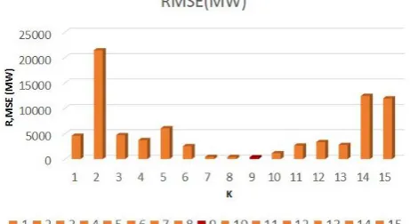
The vital part of proposed method is to determine the size of observation time window. In experimental test, the size k
which represents the number of points nearest to xs of
observation time window is to set up from 1 to 15 for finding out the best size k of train data xt to minimize forecasting error.
According to the fifteen results of best size k, and the results are shown in figure 5-1 and figure 5-2, the error rate of MAPE and RMSE is lowest when k equals 9. Due to that experimental test is based on a case study of summer period data, so the best k of summer period is 9.
[image:3.595.313.544.57.183.2]Fig 1. MAPE of proposed adaptive ARIMA model with different size of observation window.
Fig 2. RMSE test of proposed adaptive ARIMA model with different size of observation window.
A.Forecasting accuracy evaluation
This part is the evaluation by comparing proposed adaptive ARIMA, conventional adaptive ARIMA with constant forgetting factor and non–adaptive ARIMA, and the training is based on summer period data (case data-1).
Figure 3. Comparison between conventional adaptive ARIMA, proposed adaptive ARIMA and conventional non-adaptive ARIMA.
[image:3.595.302.545.290.484.2]The MAPE of proposed adaptive ARIMA model is 3.117601044 % that is lower than the conventional adaptive ARIMA model. That means the proposed adaptive ARIMA model is better than conventional RLS-forgetting factor method, and improves 84.821% in MAPE and 75.073% in RMSE error evaluation.
Table I MAPE & RMSE OF THREE METHODS UNDER SUMMER PERIOD
Conventional Adaptive ARIMA(0.99)
Proposed Adaptive ARIMA(K=9)
Conventional Non-adaptive
ARIMA MAPE (%) 5.76195944754 3.117601044 7.423626457 RMSE (MW) 630.7553231 360.280489 731.9617385
[image:3.595.56.280.521.661.2] [image:3.595.303.555.617.682.2]Figure 4. MAPE of conventional adaptive ARIMA, proposed adaptive ARIMA and conventional non-adaptive ARIMA in summer period.
Figure 5. RMSE of conventional adaptive ARIMA, proposed adaptive ARIMA and conventional non-adaptive ARIMA in summer period.
B. Stability evaluation of proposed method
For the evaluation of proposed method’s forecasting accuracy stability or robustness, training proposed adaptive ARIMA model with spring period data (case data-2).
Figure 6. MAPE of conventional adaptive ARIMA, proposed adaptive ARIMA and conventional non-adaptive ARIMA in spring period
Figure 7. RMSE of conventional adaptive ARIMA, proposed adaptive ARIMA and conventional non-adaptive ARIMA in spring period
Table II. MAPE & RMSE OF PROPOSED METHOD (k=8) Proposed Adaptive
ARIMA(K=8) MAPE (%) 1.88668354394 RMSE (MW) 187.134295961
The best k is 8 according to the figures above, and establishing model with that k. The train performance is robust both in summer time and spring time. In the same quarter, the patterns of power fluctuations are similar, so we could set up the observation window and use it during each quarter that means there are different values of k during different quarter.
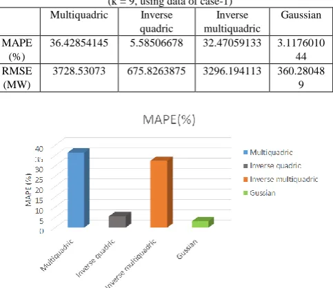
C. Evaluation of weight measure effect on accuracy
For the evaluation by comparing proposed adaptive ARIMA with variable weight based on different type RBF, since the RBF includes Multiquadric, Inverse quadric, Inverse multiquadric and Gaussian. It is necessary to find which RBF is the best measurement of weight with the summer time train data.
[image:4.595.330.523.63.113.2]The experimental results show that Gaussian RBF that is used in proposed method has the best performance compared with others.
Table III. MAPE & RMSE OF DIFFERENT ALGORITHMS (k = 9, using data of case-1)
Multiquadric Inverse quadric
Inverse multiquadric
Gaussian MAPE
(%)
36.42854145 5.58506678 32.47059133 3.1176010 44 RMSE
(MW)
[image:4.595.61.278.224.376.2]3728.53073 675.8263875 3296.194113 360.28048 9
[image:4.595.304.546.375.584.2]Figure 8. RMSE of Multiquadric, Inverse quadric, Inverse multiquadric and Gaussian RBF
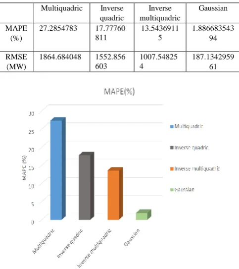
[image:4.595.59.271.466.586.2] [image:4.595.56.272.629.761.2] [image:4.595.316.537.647.735.2]In addition, the different weight measure is applied into spring period to test the accuracy. The experimental results show that Gaussian RBF that is used in proposed method has the best performance compared with others.
[image:5.595.48.290.183.455.2]The results are showed that the Gaussian function has the best performance compared with other functions, and Gaussian function has good robustness both in spring and summer period.
Table IV. MAPE & RMSE OF DIFFERENT ALGORITHMS (k = 8, using data of case-2)
Multiquadric Inverse quadric
Inverse multiquadric
Gaussian MAPE
(%)
27.2854783 17.77760 811
13.5436911 5
1.886683543 94 RMSE
(MW)
1864.684048 1552.856 603
1007.54825 4
187.1342959 61
Figure 10. RMSE of Multiquadric, Inverse quadric, Inverse multiquadric and Gaussian RBF (case-2, spring period)
Figure 11. RMSE of Multiquadric, Inverse quadric, Inverse multiquadric and Gaussian RBF (case-2, spring period)
V. CONCLUSION
This paper proposes a novel method of adaptive ARIMA compared with conventional adaptive ARIMA. The experimental results show the advanced performance of proposed method. Because there is little fluctuation in daily electric load during the same quarter, selecting fixed observation for each quarter is acceptable. Moreover, the parameters of ARIMA model could be updated with the forecasting of each points.
The proposed method improves 84.821% in MAPE and 75.073% in RMSE error evaluation compared with conventional adaptive ARIMA that is based on the training of summer data. In addition, the proposed method also need to be trained with other city’s data to test the robustness in the future work.
ACKNOWLEDGMENT
Thanks for the supervisor Prof. MURATA who is my tutor, guide, and give my research valuable advice. The case study shows the train performance and advantages of my proposed method. In addition, I want to thank the help of my friends in Waseda University.
REFERENCES
[1] Carlo Cecati, Janusz Kolbusz, A novel RBF training algorithm for short-term electric load forecasting and comparative studies. IEEE Transaction on Industrial Electronics (Volume: 52, Issue: 10, Oct. 2015)
[2] Mohamed E. EI-hawary. The Smart Grid-State of the Art and Future Trends. Pages 239-250. 19, Nov 2013. Electric Power Components and System.
[3] W.J.N.Turner, I.S. Walker, J.Roux. Peak load reductions: Electric load shifting with mechanical pre-cooling of residential buildings with low thermal mass. Feb, 2015. Volume 82, 15 March 2015, Pages 1057-1067, Energy.
[4] Etimad Fadel, V.C. Gungor, Laila Nassef, Nadine Akkari, M.G. Abbasa Malik, Suleiman Almasri, Ian F. Akyildiz. Volume 71, 1 November 2015, Pages 22-23. Computer Communications.
[5] Hao Quan, Dipti Srinivasan, Abbas Khosravi. Short-term load and wind power forecasting using neural network-based prediction intervals. (Volume: 25, Issue 2, Feb.2014). IEEE Transactions on Neural Networks and Learning Systems.
[6]Shu-Hung Leung, Gradient-based variable forgetting factor RLS algorithm in time-varying environments. IEEE Transactions on Signal Processing (Volume: 53, Issue 8, Aug.2005). 18 July 2005, pp. 3141–3150.
[7] Constantin Paleologu, Jacob Benesty, Silviu Ciochina. A Practical Variable Forgetting Factor Recursive Least-Squares Algorithm. Electronics and Telecommunications (ISETC), 2014 11th International
Symposium on. 15 January 2015.
[8]Constantin Paleologu, Jacob Benesty, Silviu Ciochina. A Robust Variable Forgetting Factor Recursive Least-Squares Algorithm for System Identification. IEEE Signal Processing Letters. 07 October 2008 (Volume: 15). Pages: 597-600.
[9] Hiroki Nakayama, Shingo Ata, Ikuo Oka. Predicting Time Series of Individual trends with Resolution Adaptive ARIMA. 14 November 2013.
[image:5.595.49.287.492.631.2]