Understanding the Solar System with Numerical Simulations and Lévy Flights

Understanding the Solar System with

Numerical Simulations and L´

evy Flights

Thesis by

Benjamin F. Collins

In Partial Fulfillment of the Requirements for the Degree of

Doctor of Philosophy

CA

L

IF

O

R

N

IA

IN

ST

ITUTE OF

T

E

C

H

N

O

L

O

G

Y

1891

California Institute of Technology Pasadena, California

2009

c

Acknowledgements

This work, literally, would not have been possible without my adviser, Re’em Sari. Collaborating with Re’em was a constantly enlightening process, and I’m very grateful for his attention, patience, and generosity as we worked together for the last six years.

Margaret Pan has been a great mentor ever since I joined her and Re’em in studying planetary dynamics. Hilke Schlichting has been an invaluable compatriot through all of our academic rites. While working and traveling with Re’em, Margaret, and Hilke, I have had many terrific adventures that I will always remember fondly.

I would like to thank my committee: Marc Kamionkowski, Shri Kulkarni, and Dave Stevenson. In addition to their roles in the preparation and defense of this thesis, I have benefited greatly from interacting with each of them in classrooms, meeting rooms, or impromptu conversations.

Abstract

This thesis presents several investigations into the formation of planetary systems and the dynamical evolution of the small bodies left over from this process.

We develop a numerical integration scheme with several optimizations for studying the late stages of planet formation: adaptive time steps, accurate treatment of close encounters between particles, and the ability to add non-conservative forces. Using this code, we simulate the phase of planet formation known as “oligarchic growth.” We find that when the dynamical friction from planetesimals is strong, the annular feeding zones of the protoplanets are inhabited by not one but several oligarchs on nearly the same semimajor axis. We systematically determine the number of co-orbital protoplanets sharing a feeding zone and the width of these zones as a function of the strength of dynamical friction and the total mass of the disk. The increased number of surviving protoplanets at the end of this phase qualitatively affects their subsequent evolution into full-sized planets.

We also investigate the distribution of the eccentricities of the protoplanets in the runaway growth phase of planet formation. Using a Boltzmann equation, we find a simple analytic solution for the distribution function followed by the eccentricity. We show that this function is self-similar: it has a constant shape while the scale is set by the balance between mutual excitation and dynamical friction. The type of evolution described by this distribution function is known as a L´evy flight.

Contents

Acknowledgements iii

Abstract iv

List of Figures viii

List of Tables x

1 Introduction and Overview 1

1.1 Numerical Code . . . 1

1.2 Co-Orbital Oligarchy . . . 3

1.3 Shear-Dominated Protoplanetary Dynamics . . . 3

1.4 L´evy Flights of Circular Binary Orbits . . . 5

1.5 Stellar Perturbations and Galactic Tides Demystified . . . 6

2 A New Planetary Simulation Code: RKNB3D 8 2.1 The Differential Equations . . . 9

2.2 The Algorithms . . . 11

2.3 Enhancements . . . 12

2.4 Numerical Tests . . . 13

2.5 Conclusions . . . 18

3 Co-Orbital Oligarchy 19 3.1 The Three-Body Problem . . . 20

3.2 The Damped N-Body Problem . . . 24

3.3 Oligarchic Planet Formation . . . 27

3.4 The Equilibrium Co-Orbital Number . . . 29

3.5 Isolation . . . 34

3.6 Conclusions and Discussion . . . 35

4 Protoplanet Dynamics in a Shear-Dominated Disk 40 4.1 Shear-Dominated Cooling and Heating Rates . . . 41

4.1.1 Eccentricity Excitation of Protoplanets . . . 42

4.1.3 Planetesimal Interactions . . . 44

4.1.4 Inclinations . . . 44

4.1.5 The Eccentricity Distribution — a Qualitative Discussion . . . 44

4.2 A Boltzmann Equation . . . 45

4.2.1 The Solution . . . 46

4.3 Numerical Simulations . . . 46

4.3.1 Equal Mass Protoplanets . . . 47

4.3.2 Mass Distributions . . . 48

4.4 Conclusions . . . 50

4.5 Appendix: The Analytic Distribution Function . . . 52

5 Self-Similarity of Shear-Dominated Viscous Stirring 54 5.1 The Time-Dependent Boltzmann Equation . . . 54

5.2 The Self-Similar Distribution . . . 56

5.3 The Generalized Time-Dependent Distribution . . . 57

5.4 Numerical Simulations . . . 59

5.5 Discussion . . . 62

6 L´evy Flights of Binary Orbits Due to Impulsive Encounters 64 6.1 A Single Encounter . . . 65

6.1.1 Close Encounters . . . 67

6.1.2 Distant Encounters . . . 67

6.1.3 Collisions . . . 68

6.2 Boltzmann Equation . . . 68

6.2.1 Eccentricity . . . 68

6.2.2 Inclination . . . 71

6.3 A Spectrum of Colliding Perturbers . . . 72

6.3.1 γ <2 . . . 72

6.3.2 γ= 2 . . . 73

6.3.3 2< γ <3 . . . 73

6.3.4 Collisional Perturbations . . . 74

6.3.5 Eccentricity Distributions . . . 75

6.4 Kuiper Belt Binaries . . . 76

6.4.1 Perturbations by a Disk . . . 76

6.4.2 Pluto et al. . . 77

6.4.2.1 Orbital Model of Tholen et al. . . 78

6.4.2.3 Theoretical Distribution . . . 81

6.4.3 Other Interesting KBOs . . . 83

6.5 Other Binary Systems . . . 84

6.6 Conclusions . . . 85

6.7 Appendix . . . 87

7 A Unified Theory for the Effects of Stellar Perturbations and Galactic Tides on Oort Cloud Comets 89 7.1 A Single Stellar Passage . . . 90

7.2 L´evy Flight Behavior . . . 91

7.3 Connection to Galactic Tides . . . 94

7.4 Conclusions . . . 101

List of Figures

2.1 RMS errors in the orbital phase of a test particle with e = 0.25 integrated with RKNB3D and Mercury, using 100 and 300 force evaluations per orbit . . . 14 2.2 RMS error in the orbital phase of a test particle withe= 0.5 integrated with RKNB3D

and Mercury, using 300 force evaluations per orbit. . . 16 2.3 RMS error in the eccentricity vector in integrations of two small protoplanets

inte-grated with RKNB3D with an average of 1 and 7 force evaluations per orbit; the relative change in total energy of the system in the integration with RKNB3D and with Mercury. . . 17

3.1 Change in semimajor axis after a conjunction of two bodies on initially circular orbits as a function of the initial separation. . . 22 3.2 Histogram of the intragroup and intergroup separations between protoplanets in

nu-merical simulations with different initial spacings. . . 26 3.3 Semimajor axes of protoplanets over time in a simulation of oligarchic growth. . . . 28 3.4 FinalhNiof simulations against the initialhNifor Σ/σ= 0.1. . . 30 3.5 Final average mass ratio, hµi, of the protoplanets plotted against the final hNi for

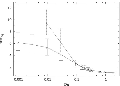
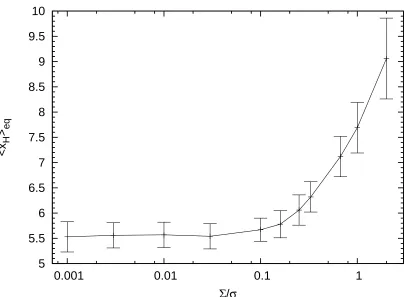
the ratio of surface densities of Σ/σ= 0.1. . . 31 3.6 Equilibrium average co-orbital numberhNieqplotted against the surface mass density

ratio of protoplanets to planetesimals, Σ/σ. . . 32 3.7 Equilibrium average spacing between co-orbital groups,hxHieq for simulations with

hNii=hNieq plotted against the surface mass density ratio Σ/σ. . . 33

3.8 Average mass of a protoplanet in an equilibrium oligarchy as a function of the surface mass density ratio Σ/σata= 1 AU. . . 34

4.1 Analytic distribution function of protoplanet eccentricities compared with the distri-bution function measured from a numerical simulation and a Rayleigh distridistri-bution. . 48 4.2 Distribution function of protoplanet eccentricities in a disk with a bimodal mass

distribution. . . 50

5.1 Eccentricity distribution of a disk of planetesimals and no dynamical friction at three different times. . . 60 5.2 The combined eccentricity distribution function of a protoplanetary population at

6.1 Illustration of the notation used to denote the geometry of a single perturbation. . . 66 6.2 Distance of Nix and Hydra from the Pluto-Charon barycenter, in units of Pluto radii,

as a function of time, in an integration of the parameters found by Tholen et al. (2008). 79

7.1 Contours of constant angular momentum on the space of possible impact parameters; the PDF of the single perturbations in thexdirection. . . 97 7.2 Marginal distribution functions of two components of the angular momentum as a

List of Tables

Chapter 1

Introduction and Overview

Astronomy was born as the first scientists, in ancient times, meticulously tracked the motion of the planets across the sky. As technology has improved, ever distant regions of the universe have become accessible, revealing a diverse menagerie of objects with fascinating properties. However, there is still much to learn about the solar system itself. We can now catalogue the tiny denizens of the outer regions of the solar system and study the orbits of their smaller satellites. We routinely leverage enormous computational power to contemplate the formation of planetary systems from the primordial dust and gas. Robotic explorers have been sent to the other planets and their moons to return in-depth measurements and high resolution images. After all this time, new data still raises new questions and the scientific frontier is pushed forward.

The work presented in this thesis focuses on understanding the processes that created the planets of our solar system. We developed a numerical code to simulate the orbital evolution of the solid bodies that eventually grow into planets. Analytic studies of the dynamics of these objects enrich the numerical work by providing a more complete understanding of the interactions of the protoplanets with themselves and the rest of the disk. Debris left over from the planet formation process exists today in the Kuiper Belt and Oort Cloud; further analytic work examines the processes that shape the orbits of these bodies in the time after the solar system formed. Understanding the evolution of their orbits allows us to determine how the conditions during their formation can be deduced from their current properties.

1.1

Numerical Code

error in the total energy due to the discretization of the integration is bounded. The equations can then be evolved with a much larger time step than in a conventional integration scheme, however the time step must remain fixed throughout the calculation. This is a significant disadvantage in certain contexts where the required time resolution may vary a great deal (a very close passage of two bodies, or modeling multiple orbits with a wide range of orbital periods). Much work has addressed these issues. Mercury (Chambers, 1999) and SyMBA (Duncan et al., 1998) are two symplectic codes that allow close encounters between the particles. Saha & Tremaine (1994) introduced a symplectic algorithm that allows each particle to have its own time step.

As part of the work presented in this thesis, we developed a new integration scheme that is designed to handle the technical problems inherent in studying the later stages of planet formation. Because it is the collisions between protoplanets that lead to their growth, it is essential that our code treats close encounters accurately. The code must be able to account for the growth of the eccentricities of protoplanets to very large values as they excite each other. Lastly, we require the capability to add extra terms to the orbital evolution in a simple way, with the intent of representing the influence of the planetesimals not through a separate integration, but by including their average effects analytically in the equations of motion of the protoplanets.

We choose special variables to minimize the error associated with discretizing the continuous physical system. Instead of describing the motion of each particle with Cartesian coordinates and velocities, we integrate constants of the two-body solution of each particle around the central mass. The central acceleration is then implicitly accounted for, and integration handles only the perturba-tions caused by interparticle forces. We employ a fifth-order Runge-Kutta algorithm with adaptive time steps (Cash & Karp, 1990; Press et al., 1992), and use a Newton-Raphson algorithm to solve Kepler’s equation. By using an adaptive time step algorithm, we achieve the stated goal of handling phenomenon that occur over a range of timescales. The simplicity of the equations easily allows the specification of non-gravitational forces. For close encounters, we use the same differential equations to integrate the relative motion of the two bodies and the orbit of their center of mass around the central star.

1.2

Co-Orbital Oligarchy

Chapter 3 presents numerical studies of the oligarchic phase of a protoplanetary disk. In this phase, proposed by Lissauer (1987) and studied by Kokubo & Ida (1998), the runaway growth of the protoplanets has left their number density low enough that they no longer experience frequent collisions. Each protoplanet then holds court over a thin annulus of the disk, and grows only by accreting nearby planetesimals. This shuts off runaway growth; the protoplanets spend most of their formation time in this phase. Occasionally, the protoplanets grow too large for their spacing to be dynamically stable. They then enter a period of chaotic close encounters. When collisions have lowered the number density of protoplanets enough, the oligarchs settle into a new stable configuration. At some point in the evolution of the disk, a stable configuration does not exist, and the protoplanets undergo a final round of strong interactions before ending up with close to their final mass (Goldreich et al., 2004a).

The dynamical friction from planetesimals is an important part of this process. Kokubo & Ida (1996, 1998) included the planetesimals explicitly in their simulations, however their planetesimals had to be large to keep the total particle number low enough to be computationally feasible. With our new simulation code, we include the effects of the planetesimals on the protoplanets without having to calculate the orbits of each individual body. This lets us study the oligarchic phase of planet formation in a more highly-damped regime.

Our simulations show that after a period of excitation, one or more protoplanets in the resulting oligarchy orbit stably at nearly the same semimajor axis. Just as collisions bring the disk towards stability by reducing the number density, the co-orbital resonances prevent those protoplanets from undergoing close encounters with each other. In Chapter 3, we present a suite of simulations to explore systematically the typical number of co-orbital oligarchs as a function of the total protoplanet mass and the strength of the dynamical friction (given by the total mass of planetesimals). A significant number of co-orbital protoplanets qualitatively changes the relationship between the oligarchic disk and the final planets. In the inner solar system, dividing the available solids into a higher number of co-orbital protoplanets decreases the mass of each one. In the giant impact phase that follows oligarchy, more collisions are then required to assemble the final terrestrial planets. In the outer solar system, where the planets reach their final size during the oligarchic phase, an enhancement of the disk is necessary to provide the material for the extra co-orbital protoplanets.

1.3

Shear-Dominated Protoplanetary Dynamics

rate depends on the relative velocities of the interacting objects, and the velocity dispersion is in turn set by the distribution of sizes of the protoplanets and planetesimals. In a Keplerian disk, the velocity dispersion is related to the eccentricity distribution: particles with some eccentricity have an extra motion on top of the background rotation of the disk.

Much previous work has sought analytic descriptions of the rates of accretion and eccentricity evolution. One technique, summarized by Stewart & Ida (2000), is to calculate average diffusion coefficients that describe the time derivative of the root-mean-squared eccentricity of the protoplanets or planetesimals.

In Chapters 4 and 5, we present a different approach to studying the eccentricities of the proto-planets. We calculate the probability density of the protoplanets’ eccentricities given the dissipation of dynamical friction and the stochastic mutual excitations. We use a Boltzmann equation that relates the probability for a single perturbation to the full distribution function of the eccentricity. In spite of the complex nature of the multi-body dynamics in the protoplanetary disk, we find an astonishingly simple analytic solution for the distribution function when the balance between mutual excitations and dynamical friction allows a steady state. The probability of finding a protoplanet in a logarithmic interval ofeis exactly:

dn(e)

dloge =

(e/ec)2

(1 + (e/ec)2₎3/2. (1.1)

This function has a peak around e ≈ ec, which corresponds, to an order of magnitude, to the eccentricity at which the timescale for dynamical friction is equal to the timescale for excitation. Aboveec, the distribution function decreases ase−1_{; the mean of the distribution is logarithmically}

divergent, and the variance is undefined.

The full distribution of eccentricities allows us to make several conclusions. The overall shape of the distribution, a two-dimensional Cauchy distribution, is qualitatively different than the Rayleigh distribution that is commonly assumed in the literature; Rayleigh distributions fall exponentially at high eccentricity while our findings show a power law behavior. The typical kinetic energy, which scales ase2_{, is dominated then by the fewer protoplanets with the highest eccentricities, while most}

of the protoplanets have eccentricities of aboutec. Numerical simulations using the code described in Chapter 2 verify the analytic solution.

Sun. Assuming a self-similar solution, the Boltzmann equation reduces to two equations that specify the distribution function. The first is a dimensionless version of the Boltzmann equation, whose solution is the shape described by Equation 1.1. The second is an ordinary differential equation that relates the rate of change of the eccentricity scale, ˙ec(t), to the damping and excitation timescales. When dynamical friction is included, this ODE reproduces the results of Chapter 4: ecis constant and set by the equilibrium between dynamical friction and protoplanet stirring. If there is no damping,ec grows linearly, and the shape of the distribution is maintained while it moves to higher values of eccentricity. Thus Equation 1.1 is an accurate description of the eccentricities of the protoplanets for both steady-state and dynamically evolving scenarios. The time-dependent scale ec(t) handles the evolution of the physical parameters, such as the surface densities. Again, numerical

simulations of this process provide a stunning verification of the analytic results.

1.4

L´

evy Flights of Circular Binary Orbits

The Kuiper belt is a collection of icy bodies outside of Neptune’s orbit that contains leftover plan-etesimals from planet formation in the outer solar system; Pluto is one of its most famous members. Recent high resolution imaging has shown Pluto to be surrounded by two very small moons in addition to its larger partner Charon (Weaver et al., 2006). Further observations constraining the orbits of the satellites show that all three have small but finite eccentricities (Tholen et al., 2008). Several other Kuiper belt objects of about the size of Pluto have been discovered and found to have nearly circular satellites of their own (Brown et al., 2005, 2006). For most of these systems, tidal interactions between the primary and the satellites are expected to damp the eccentricity of the satellites, leaving their orbits completely circular.

Close approaches by other Kuiper belt objects (KBOs) are one possible source for the eccentricity of these systems. Stern et al. (2003) studied the forcing of the eccentricity of Pluto-Charon with a numerical experiment simulating random encounters from other KBOs. They found that the observed eccentricity of 0.003 is too large to be explained by the stochastic perturbations, given the theoretical estimate of the eccentricity damping rate.

L´evy flights to solve for the distribution function of the binary’s eccentricity for perturbing mass distributions of arbitrary power law slopes.

From the distribution function for the eccentricity of these systems we calculate confidence inter-vals for an observed eccentricity, given the mass distribution of the Kuiper belt. The eccentricities of the outer two satellites of Pluto are within these intervals. The eccentricity of Charon, on the other hand, is too large to be attributed to impulsive perturbations. The eccentricities of the satellites of the other two Plutoids, Eris, and Haumea, are consistent with external perturbations if tidal dissipation is ignored.

1.5

Stellar Perturbations and Galactic Tides Demystified

Another possible fate for the leftover planetesimals is that they become the Oort cloud of comets. At the end of planet formation, the perturbations from the new planets add energy to the planetesimals, but their periapses remain in the planetary region. Thus their eccentricity grows close toe= 1. Once the semimajor axes of the comets get large enough, perturbations from passing stars in the Galaxy begin to affect the orbits of the comets. Their periapses grow, saving them from the planetary perturbations and trapping them in what is called the Oort cloud. When the orbits of the small bodies evolve back into the planetary region, we observe them as comets.

Heisler & Tremaine (1986) found that the planar mass distribution of the Galactic disk exerts a torque on the comet that dominates the effects of stellar encounters over long timescales. Subsequent numerical studies of the formation of the Oort cloud have included both a mean growth of the magnitude specified by the Galactic tides and a stochastic term to represent stellar perturbations (Duncan et al., 1987; Heisler, 1990; Dones et al., 2004).

We tackle this problem with the techniques developed in the previous chapters. First we examine the perturbations caused by a single field star traveling on a straight trajectory. We then relate the spectrum of possible single perturbations to the distribution function of the comet’s angular momentum. Amusingly, the angular momentum vector also follows a L´evy flight. The shape of the distribution function is the two-dimensional Cauchy distribution, and the typical value is set by a differential equation that depends on the parameters of the comet and the perturbing swarm. These similarities to the nearly circular case are a consequence of the identical scaling of the perturbation strength with the mass of a single perturber, its distance of closest approach to the comet, b, and its velocity,vp.

preferentially to one component of the total angular momentum vector. The coherent accumulation from these perturbations causes the angular momentum vector to grow, on average, in one direction. This effect is exactly the torque derived from the smooth planar mass distribution and attributed to the tides from the Galactic disk.

Chapter 2

A New Planetary Simulation Code: RKNB3D

In 1991, Wisdom & Holman revolutionized planetary dynamics. The symplectic integrators that they developed evolve the orbital equations of motions exactly under a Hamiltonian close to but different from the Hamiltonian of the physical system. The difference between the physical Hamiltonian and the numerical one represents the truncation error of the calculation. This error is typically bounded and does not accumulate throughout the integration. Accordingly, a symplectic integration can be carried out with a much larger time step than is possible when using a conventional integration scheme.

One downside is that the time step of a symplectic integrator must remain fixed throughout the calculation. In some contexts a fixed time step is not a problem, such as a long-term simulation of the outer solar system (Duncan & Quinn, 1993). In planet formation, however, there are occasional events that must be integrated with time steps much shorter than is necessary during the majority of the simulation. The acceleration experienced by very eccentric particles is stronger near periapse and weaker at apoapse, and this ratio can be extreme. Pairs of bodies often pass close enough to each other that their mutual gravitation is stronger than that from the star, but the encounters usually last less than a single orbital period. Setting the time step of the entire simulation to resolve these quick and isolated events reduces the efficiency of symplectic techniques.

Many authors have developed symplectic codes that address these problems. Saha & Tremaine (1994) devised an algorithm in which the time step of each particle is set independently; however the time step does not adapt in response to the events in the simulation, so this is not an ideal solution for the two problems mentioned above. SyMBA (Duncan et al., 1998) and Mercury (Chambers, 1999) are two codes that implement methods to integrate close encounters without interfering with the energy conservation of the overall integration.

In Section 2.4 we test the performance of our code and compare its properties to several symplectic codes. We summarize our results in Section 2.5.

2.1

The Differential Equations

The most naive way to calculate the orbits of many gravitationally interacting particles is to integrate the changes in their positions and velocities directly. In the context of planetary systems, such a scheme overlooks the integrability of the two-body system. Specifically, the shape of the orbit of a single particle around a central mass is given by a closed-form analytic expression. Directly integrating the acceleration from the star introduces errors that, in a two-body system, are entirely avoidable. In our code, we integrate a set of osculating orbital elements instead of the positions and velocities. These parameters describe the solution to the two-body problem that each particle would follow if there were no accelerations besides that from the central object. Compared to the size of the central acceleration, the other perturbations are, typically, orders of magnitude smaller.

Our criterion for choosing the orbital elements to integrate is that they are well-behaved. We avoid the longitude of periapse and the longitude of the ascending node, since for circular non-inclined orbits they are not defined. More importantly, if the eccentricity and inclinations are small, small perturbations may change these angles by a large amount, forcing the integration algorithm to take more time steps than would otherwise be required.

Our code tracks nine parameters for each body: the energy per unit mass,E, the two-dimensional eccentricity vectore, the three-dimensional angular momentum per unit mass,H, the current mod-ified eccentric anomaly, ¯E(t), the modified eccentric anomaly at a reference time, ¯E0, and the mass

of the particle, m. Since these quantities are constants of the two body solution, the only time derivatives that do not cancel to first order are those due to the interparticle accelerations, which we denoteA. The energy per unit mass,E, evolves as:

˙

E=A·v. (2.1)

The derivative of the energy is the work done by all the other particles. The eccentricity vector,e= (v_×H)/G(Mc+m)−r, evolves as:ˆ

˙

e=

₁

G(Mc+m)

[2r(v_·A)−v(r_·A)−A(r_·v)]. (2.2)

The derivative of the angular momentum per unit mass vector,H, is the torque:

˙

H=r×A. (2.3)

This three-dimensional vector is integrated relative to a fixed coordinate system. It describes the orientation of the orbital plane in a more well-behaved way than the inclination angle and the line of nodes. Also, we can use its components to transform the position and velocities of the particles into and out of the orbital plane.

The modified eccentric anomalies, ¯E and ¯E0, are used in a version of Kepler’s equation to find

the phase of the particle as a function of time, given the rest of its orbital parameters.

n(t−t0) = ¯E−E¯0−e1(sin ¯E−sin ¯E0) +e2(cos ¯E−cos ¯E0), (2.4)

wheren= (−2E)3/2_{/G(Mc+m) is the orbital frequency,e}

1and e2are the components ofein the

orbital plane, and ¯E0 = ¯E(t=t0). This version of Kepler’s equation is derived from the usual one

by combining the eccentric anomaly with the longitude of periapse, ¯E=E+̟. Finding the phase by solving Kepler’s equation is an alternative to integrating the phase itself over time, which would have caused errors to accumulate even when calculating the constant orbit of a single particle.

Instead of using the time of last periapse passage as a two-body constant of motion, we use the modified eccentric anomaly ¯E0, which is also constant for a two-body system. The formula for ˙¯E0

is tedious to derive. The derivative of Equation 2.4 provides most of the terms, and we use the derivative ofxsin ¯E−ycos ¯E to solve for ˙¯E, wherexand y are the components ofrin the orbital plane and are a function of ¯E.

Unfortunately, the expression for ˙E¯0 contains a term proportional to t. To reduce the effect

this has on the integration, we update t0 and ¯E0 periodically for each particle. This introduces an

accumulation of error with every rescaling, but at a much slower rate than a direct integration of the orbital phase.

The energy,E, the eccentricity vector, e, and the angular momentum, H, all evolve smoothly through the transition between bound and unbound orbits. Unbound orbits, however, require a different version of Kepler’s equation:

n(t−t0) =e(sinhF−sinhF0)−F+F0, (2.5)

where F and F0 are the hyperbolic anomalies at time t and t0 respectively (Danby, 1988). The

equation for ˙F0again is tedious to derive but follows from algebraic manipulation of the derivatives

of Equation 2.5 and the components ofr(F).

particle in the plane of its orbit. As noted above, the components ofHprovide the transformation between the orbital plane of each particle and the fixed frame. Since this transformation evolves as

Hevolves, the derivatives ofeand ¯E0, which are fixed in the orbital plane, must include additional

terms depending on ˙H.

Finally, we allow for the specification of an arbitrary ˙m, which, physically, could represent the average accretion rate of planetesimals onto the protoplanets in a simulation of planet formation. A time-dependent mass affects the translation between Cartesian coordinates and the elements. Physically, the elements do evolve as a result of planetesimal accretion; however, for simplicity, we set the derivatives of the other elements such that the shape of the orbit is not affected by a change in mass.

2.2

The Algorithms

Finding an efficient set of evolution equations is only part of the simulation scheme; choosing an effective algorithm to integrate them is also important. As stated before, one goal for this code is to implement adaptive time steps. Another goal is to allow the inclusion of additional accelerations to represent effects like dynamical friction that are caused by a population of bodies too numerous to be integrated. These forces can be dissipative, so we must not use algorithms that require a conservative force. Finally, we note that the most potentially computationally intensive part of our code is calculating the gravitational forces, which contributes to the total running time proportionally toN2_{, whereN is the number of particles. Thus we favor lower order codes that require fewer force}

evaluations.

We choose a fifth-order Runge-Kutta scheme with Cash-Karp coefficients (Cash & Karp, 1990; Press et al., 1992). In this algorithm, the values of the equations at the end of a time step can be estimated to any order below five using linear combinations of the same sub-step calculations. Comparing the fourth-order calculation to the full fifth-order one provides an estimate of the error in each step, which is used to adjust the size of the subsequent step. The accuracy of the integration is controlled by specifying a tolerance for the errors of each step. Since we anticipate our param-eters to have small values, we use the absolute error of each variable to adjust the step size. Our implementation of this algorithm is based on the description by Press et al. (1992).

2.3

Enhancements

One advantage of this scheme is that it implicitly evolves the particles under the acceleration from the central mass, which typically provides the largest acceleration by several orders of magnitude. This hierarchy is reversed, however, when two particles suffer a very close encounter; in planet formation, these events are essential for the growth of the protoplanets and the excitation of their velocity dispersion. The distance from a particle where the motion due to the Sun is comparable to the motion caused by the gravity between the two close particles is known as the Hill radius; we use the definition thatRH= (m/(3M⊙))1/3a.

As one particle approaches another on the scale of their Hill radii, the advantages of our dif-ferential equations are lost. To accurately describe the motion of one particle around the other, the constants of motion of the heliocentric two-body solution must undergo large rapid changes. However, in the limit that the particles are very close to each other, their relative motion is very close to a two-body solution, with the central star providing only a perturbation. We follow the objects through the close encounter by using the same differential equations to integrate the shape of the relative orbit. The center of mass of the pair of particles is not affected by their strong mutual acceleration, and is described well by a two-body solution around the central star.

Another coordinate transformation is necessary to handle the transition between bound and unbound orbits. Since the shape of bound and unbound orbits are fundamentally different, each regime requires its own conversion between the two-body constants of motion and the position of the particle. We implement a transition region in the code for the particles that are in between the two regimes. We integrate the position and velocity of these particles directly, including the acceleration from the central object as well as all other particles. While this solution offends the sense of error-minimization adhered to by the rest of the code, the relative amount of time spent integrating these coordinates is very small. The benefit is the ability to smoothly integrate an orbit that undergoes almost any kind of change.

2.4

Numerical Tests

To demonstrate the performance of our code, we present three tests. The first is to monitor the Jacobi constant, an integral of the motion in the circular-restricted three-body problem. We perform the same simulations as described in Section 6.3 of Duncan et al. (1998) so that, in addition to comparing the conservation of the Jacobi constant in the two codes, we can compare the qualitative results of our simulations with theirs. We integrate 50 massless particles interacting with a Neptune-sized planet, which has been placed on a circular orbit at 30 AU. The initial coplanar orbits of the test particles are such that all 50 have periapses at 30 AU, but their semimajor axes are spread evenly between 36 and 40 AU. The integrations are carried out for 109 _{years or until the massless particle}

collides with Neptune. Since many of the test particles do collide after undergoing many close encounters with Neptune, this is a good test of our code’s ability to resolve the close encounters.

Our results are quite similar to those using the SyMBA code (Duncan et al., 1998). We find a median lifetime of the test particles of 4.5×106_{years, within about a factor of two of their results.}

The average time steps of our simulations range between 2.0 and 8.3 years, with a median of 3.8. For comparison, the SyMBA integrations used a time step of 2 years. Our worst case error in the Jacobi constant is 1 out of 14,000; again this is close to the results of SyMBA’s performance on this test. We point out that the error conservation is entirely dependent on the simulation time; particles that collided with Neptune earlier showed a much lower amount of accumulated error. The number of close encounters in a single simulation did not affect the rate of error accumulation, so we trust that our scheme for integrating close encounters has performed well.

We next examine the accumulation of error in the orbital phase of a particle, and compare it to the phase error of the same integration using the Mercury code (Chambers, 1999). This investigation is based on similar integrations comparing a variety of algorithms in Saha & Tremaine (1992). We integrate the orbit of a massless asteroid at 2.6 AU, with an eccentricity of 0.25 and an inclination of 0.2 rad. We include Jupiter with its current eccentricity and inclination. For both our code and Mercury, we perform several integrations with different levels of accuracy. By comparing the orbital phase of the asteroid in the most accurate simulation against the others, we estimate the absolute error in the orbital phase as a function of the specified time step or tolerance parameter.

To normalize the differences in the order of the two codes (RKNB3D being fifth-order and Mercury being second), we only compare the errors of simulations that use the same number of force evaluations per orbit. For RKNB3D, we divide the total number of force evaluations by the integration time to find the average number per orbit. RKNB3D has an inherent disadvantage in this metric, since our algorithm requires six force evaluations at each time step, and second-order symplectic codes require only one.

1e-07

1e-06

1e-05

1e-04

0.001

0.01

0.1

1

10

100

1000

10000

∆θ

(in radians)

Time (in orbits)

Mercury

RKNB3D

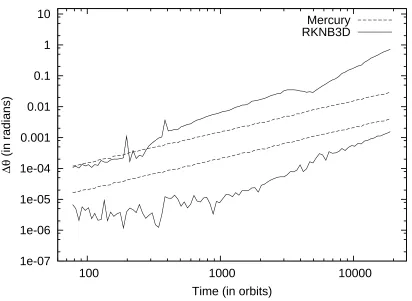
tions. The upper lines are computed from simulations with 100 force evaluations each orbit, as in Figure 1 of Saha & Tremaine (1994). Each measurement is the root-mean-square of the difference in orbital phase at several points spread across multiple orbits. The phase error of the asteroid in Mercury, the dashed line, grows linearly with time over the entire length of the integration. The asteroid in our code, in the solid line, initially shows the same level of error. However after a few hundred orbits, the error accumulation accelerates, causing the phase error to grow faster than in the Mercury integrations.

For this scenario, the symplectic integrator has lived up to its reputation. However, since RKNB3D is a higher order code than Mercury, increasing the number of force evaluations per step has a greater effect on the overall error accumulation. The lower lines in Figure 2.1 correspond to simulations with 300 force evaluations per orbit. While the error in the orbital phase of both codes has decreased, the RKNB3D simulations shows less error accumulation over the entire integration.

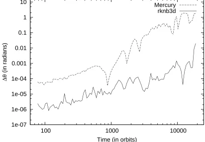
This relatively simple configuration does not thoroughly test most of the functional improve-ments included in RKNB3D. As a second trial, we increase the eccentricity of the asteroid to 0.5. These simulations reveal a large degradation in the performance of Mercury for all time steps. In simulations using 100 force evaluations per orbit, the phase error in both codes reaches order unity before the end of the integration. Using 300 force evaluations per orbit reduces the phase errors to reasonable values; the results of these simulations are plotted in Figure 2.2. Here RKNB3D exhibits less error overall as well as a similar rate of accumulation as Mercury. This improvement is likely due to the ability of RKNB3D to spend extra computational time resolving the periapse passage of the asteroid, and less time integrating the weaker perturbations at apoapse.

Our final test is a simulation of two very small protoplanets separated by about 10 Hill radii. The relative motion between these two protoplanets is slow since their orbital periods are almost equal. Their interactions occur only during conjunctions, otherwise the acceleration each provides on the other is very weak and changes very slowly. The adaptive time steps of our scheme are enormously beneficial to this configuration. The two protoplanets have mass ratios ofµ= 10−12 _of

the central star. They initially follow circular coplanar orbits, one at 1 AU and the other separated byx= 2µ2/7_{a= 0.00372759 AU. This separation was chosen to be large enough that the dynamics}

were not chaotic; chaos occurs when the separation is less than about 1.3µ2/7_{a(Wisdom, 1980). As}

in Figures 2.1 and 2.2, a reference simulation with much higher accuracy was used as the benchmark for the eccentricity vector. In this case, our reference simulation uses 126 force evaluations per orbit on average, and the maximum step size is limited to 0.016 years. We compared this reference integration to two other simulations with different tolerances and no step size limitations.

1e-07

1e-06

1e-05

1e-04

0.001

0.01

0.1

1

10

100

1000

10000

∆θ

(in radians)

Time (in orbits)

Mercury

rknb3d

10

10

10

10

10

10

∆

e

-1.5e-12

-1e-12

-5e-13

0

5e-13

1e-12

10

10

10

∆

E/E

Time (in years)

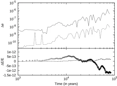
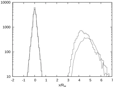
Figure 2.3 Top panel: RMS error in the eccentricity vector in integrations of two small protoplanets (µ = 10−12_{), separated by 10 R}

H, and simulated in RKNB3D with an average of 1 and 7 force

decreases to between around 0.1–0.01 years; when the bodies are apart, the time steps increase to as high as 100 years for the integration shown in the solid line. The more accurate integration, shown in the dashed line, increases the step size to only 1–2 years between conjunctions.

The bottom panel of Figure 2.3 compares the total energy conservation of the system when integrated with RKNB3D to the same system integrated in Mercury. The solid line corresponds again to the RKNB3D integration with an average of 1 force evaluation per orbit. The crosses show the performance of a Mercury integration that uses 100 force evaluations per orbit. Even though both codes conserve the error well, the accuracy of RKNB3D, even when it is taking steps of up to 100 years, demonstrates the usefulness of our numerical approach.

2.5

Conclusions

In this chapter, we have outlined a new scheme for integrating the orbits of many particles around a more massive central object. We have designed this code with several optimizations for studying planet formation, such as a robust handling of close encounters between particles, and an algorithm with adaptive time steps. Tests of its performance against popular symplectic codes have showed that it is outperforms those codes in some circumstances.

Several research projects using this code have already been completed. Chapter 3 describes a numerical study of the configuration of protoplanets in a protoplanetary disk. This study benefited greatly from the ability to include arbitrary force terms in the integration. One such term was the effect of dynamical friction caused by a population of protoplanets. We also introduced a restoring force at the edges of the simulation region. By pushing the protoplanets back in as they are scattered out, we keep their surface mass density more constant.

In Chapters 4 and 5 we present an analytic technique to study the eccentricities of protoplanets. However, to confirm our results, we perform numerical integrations to measure the distribution function of the eccentricity directly. In these simulations we placed 120 particles in a small annular region, with mass ratios of 10−10_{to 10}−8_{of the central star. With such a high number density, close}

Chapter 3

Co-Orbital Oligarchy

The early stages in the formation of planetary systems are well described by statistical calcula-tions of the evolution of mass distribucalcula-tions and velocity dispersions. As larger bodies accumulate from the swarm of protoplanetary material, their individual dynamics begin to dominate their evo-lution. Lissauer (1987) pointed out that the finite crosssection for accretion limits the growth of each protoplanet. This is now known as the “oligarchic phase.” (Kokubo & Ida, 1998). Numerical (Kenyon & Bromley, 2006; Ford & Chiang, 2007; Levison & Morbidelli, 2007) and analytical (Gol-dreich et al., 2004a) work has explored the transition from oligarchic growth to the chaotic final assembly of the planets. In this chapter we examine the interactions of a moderate number of pro-toplanets in an oligarchic configuration and find that neighboring propro-toplanets stabilize co-orbital systems of two or more protoplanets. We present a new picture of oligarchy in which each part of the disk is not ruled by one but by several protoplanets having almost the same semimajor axis.

Our approach is to systematize the interactions between each pair of protoplanets in a disk where a swarm of small icy or rocky bodies, the planetesimals, contain most of the mass. The planetes-imals provide dynamical friction that circularizes the orbits of the protoplanets. The total mass in planetesimals at this stage is more than that in protoplanets so dynamical friction balances the excitations of protoplanets’ eccentricities. We characterize the orbital evolution of a protoplanet as a sequence of interactions occurring each time it experiences a conjunction with another protoplanet. The number density of protoplanets is low enough that it is safe to neglect interactions among three or more protoplanets.

To confirm our description of the dynamics and explore its application to more realistic protoplan-etary situations we perform many numerical N-body integrations. We use an algorithm optimized for mostly circular orbits around a massive central body. As integration variables we choose six con-stants of the motion of an unperturbed Keplerian orbit. As the interactions between the other bodies in the simulations are typically weak compared to the central force, the variables evolve slowly. We employ a fourth-order Runge-Kutta integration algorithm with adaptive time steps (Press et al., 1992) to integrate the differential equations. During periods of little interaction, the slow evolution of our variables permits large time-steps.

During a close encounter, the interparticle gravitational attraction becomes comparable to the

force from the central star. In the limit that the mutual force between a pair of particles is much stronger than the central force, the motion can be more efficiently described as a perturbation of the two-body orbital solution of the bodies around each other. We choose two new sets of variables: one to describe the orbit of the center of mass of the pair around the central star, and another for relative motion of the two interacting objects. These variables are evolved under the influence of the remaining particles and the central force from the star.

Dynamical friction, when present in the simulations, is included with an analytic term that damps the eccentricities and inclinations of each body with a specified timescale. All of the simulations described in this chapter were performed on Caltech’s Division of Geological and Planetary Sciences Dell cluster.

We review some basic results from the three-body problem in Section 3.1 and describe the modifications of these results due to eccentricity dissipation. In Section 3.2, we generalize the results of the three-body case to an arbitrary number of bodies, and show the resulting formation and stability of co-orbital subsystems. Section 3.3 demonstrates that an oligarchic configuration with no initial co-orbital systems can acquire such systems as the oligarchs grow. Section 3.4 describes our investigation into the properties of a co-orbital oligarchy, and Section 3.5 places these results in the context of the final stages of planet formation. The conclusions are summarized in Section 3.6.

3.1

The Three-Body Problem

The circular-restricted planar three-body problem refers to a system of a zero mass test particle and two massive particles on a circular orbit. We call the most massive object the star and the other the protoplanet. The mass ratio of the protoplanet to the star isµ. Their orbit has a semimajor axisa and an orbital frequency Ω. The test particle follows an initially circular orbit with a semimajor axis

atp =a(1 +x) withx≪1. Since the semimajor axes of the protoplanet and the test particle are

close, the two objects rarely approach each other. For smallx, the angular separation between the two bodies changes at the rate (3/2)Ωxper unit time. Changes in the eccentricity and semimajor axis of the test particle occur only when it reaches conjunction with the protoplanet.

The natural scale for xais the Hill radius of the protoplanet, RH≡(µ/3)1/3a. For interactions

at impact parameters larger than about 4 Hill radii, the effects of the protoplanet can be treated as a perturbation to the Keplerian orbit of the test particle. These changes can be calculated analytically. To first order in µ, the change in eccentricity is ek = Akµx−2_{, where Ak = (8/9)[2K}

0(2/3) +

K1(2/3)] ≈ 2.24 and K0 and K1 are modified Bessel functions of the second kind (Goldreich &

Tremaine, 1978; Petit & Henon, 1986).

momentum per unit mass of the test particle. RewritingCJ in terms ofxande, we find that

3 4x

2

−e2= const. (3.1)

If the encounter increasese,|x|must also increase. The change inxresulting from a single interaction on an initially circular orbit is

∆x= (2/3)e2k/x= (2/3)A2kµ2x−5. (3.2)

The contributions of later conjunctions add to the eccentricity as vectors and do not increase the magnitude of the eccentricity by ek. Because of this, the semimajor axis of the test particle generally does not evolve further than the initial change ∆x. Two alternatives are if the test particle is in resonance with the protoplanet, or if its orbit is chaotic. If the test particle is in resonance, the eccentricity of the particle varies as it librates. Chaotic orbits occur when each excitation is strong enough to change the angle of the next conjunction substantially; in this case,eandxevolve stochastically (Wisdom, 1980; Duncan et al., 1989).

Orbits withxbetween 2 and 4RH/acan penetrate the Hill sphere and experience large changes in

eanda. This regime is highly sensitive to initial conditions, so we only offer a qualitative description. Particles on these orbits tend to receive eccentricities of the order of the Hill eccentricity,eH≡RH/a,

and accordingly change their semimajor axes by ∼ RH. We will call this the “strong-scattering

regime” of separations. A fraction of these trajectories collide with the protoplanet; these orbits are responsible for protoplanetary accretion (Greenzweig & Lissauer, 1990; Dones & Tremaine, 1993).

For x . RH/a, the small torque from the protoplanet is sufficient to cause the particle to

pass through x = 0. The particle then returns to its original separation on the other side of the protoplanet’s orbit. These are the famous horseshoe orbits that are related to the 1:1 mean-motion resonance. The change in eccentricity from an initially circular orbit that experiences this interaction can be calculated analytically (Petit & Henon, 1986):ek = 22/3₃−3/2_5Γ(2/3)µ1/3_{exp(−(8π/9)µx}−3_),

where Γ(2/3) is the usual gamma function. Since this interaction is very slow compared to the orbital period, the eccentricity change is exponentially small as the separation goes to zero. As in the case of the distant encounters, the conservation of the Jacobi constant requires that xincreases as the eccentricity increases (equation 3.1). Then,

∆x= 2.83µ

2/3

x exp(−5.58µx

−3_{). (3.3)}

10

10

10

10

10

10

10

10

10

10

20

10

5

2

1

∆

a/R

x/R

Horseshoe

Scattering

Strong

Distant

Encounters

10

10

10

10

10

10

10

10

10

10

20

10

5

2

1

∆

a/R

x/R

Horseshoe

Scattering

Strong

Distant

Encounters

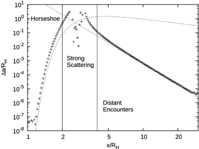
Figure 3.1 Change in semimajor axis after a conjunction of two bodies on initially circular orbits whose masses are smaller than that of the star by the ratio µ = 3×10−9_{, plotted as a function}

of the initial separation. The points are calculated with numerical integrations, while the dashed lines show the analytic results, equations 3.2 and 3.3. At the smallest impact parameters the bodies switch orbits; in this case we have measured the change relative to the initial semimajor axis of the other protoplanet. The horizontal lines separate the regions ofxthat are referred to in the text.

3.3 withµ=µ1+µ2.

Figure 3.1 plots the change in aafter one conjunction of two equal mass protoplanets as mea-sured from numerical integrations. All three types of interactions described above are visible in the appropriate regime ofx. Each point corresponds to a single integration of two bodies on initially cir-cular orbits separated byx. For the horseshoe-type interactions, each protoplanet moves a distance almost equal tox; we only plot the change in separation: ∆aH.S.=|∆a| − |x|a. The regimes of the three types of interactions are marked in the figure. The dashed line in the lowxregime plots the analytic expression calculated from equation 3.3. The separations that are the most strongly scat-tered lie between 2−4RH, surrounding the impact parameters for which collisions occur. For larger

separations the numerical calculation approaches the limiting expression of equation 3.2, which is plotted as another dashed line.

At the same time, the planetesimals provide dynamical friction that damps the eccentricities of the protoplanets. When the typical eccentricities of the protoplanets and the planetesimals are lower than the Hill eccentricity of the protoplanets, this configuration is said to be shear dominated: the relative velocity between objects is set by the difference between the orbital frequency of nearby orbits. In the shear-dominated eccentricity regime, the rate of dynamical friction is (Goldreich et al., 2004b):

−1

e de

dt =Cd

σΩ

ρRα

−2₌ 1

τd

, (3.4)

whereRandρare the radius and density of a protoplanet,σis the surface mass density in planetes-imals,αis the ratioR/RH, andCd is a dimensionless coefficient of order unity. Recent studies have

found values for Cd between 1.2 and 6.2 (Ohtsuki et. al. 2002; H. Schlichting and R. Sari, private communication). For this work, we use a value of 1.2. For parameters characteristic of the last stages of planet formation, τd ≫2π/Ω. The interactions of the protoplanets during an encounter are unaffected by dynamical friction and produce the change in e and a as described above. In between protoplanet conjunctions, the dynamical friction circularizes the orbits of the protoplanets. The next encounter that increasesefurther increasesxto conserve the Jacobi constant. The balance between excitations and dynamical friction keeps the eccentricities of the protoplanets bounded and small, but their separation increases after each encounter. This mechanism for orbital repulsion has been previously identified by Kokubo & Ida (1995), who provide a timescale for this process. We alternatively derive the timescale by treating the repulsion as a type of migration in semimajor axis. The magnitude of the rate depends on the strength of the damping; it is maximal if all the eccentricity is damped before the next encounter, or τd ≪4π/(3Ωx). In this case, a protoplanet with a mass ratio µ1and semimajor axisa1 interacting with a protoplanet with a mass ratioµ2 in

the regime of distant encounters is repelled at the rate:

1 a1

da1

dt =

A2

k

2πµ2(µ1+µ2)x

−4_{Ω. (3.5)}

For protoplanets in the horseshoe regime, the repulsion of each interaction is given by equation 3.3. These encounters increase the separation at an exponentially slower rate of:

1 a1

da1

dt = 0.67µ2(µ1+µ2)

−2/3_exp(

−5.58(µ1+µ2)x−3)Ω. (3.6)

whereτd≪4π/(3Ωx).

3.2

The Damped N-Body Problem

Having characterized the interactions between pairs of protoplanets, we next examine a disk of protoplanets with surface mass density Σ. Each pair of protoplanets interacts according to their separations as described in Section 3.1. If the typical spacing is of orderRH, the closest encounters

between protoplanets cause changes in semimajor axes of aboutRHand eccentricity excitations to

eH. The strong scatterings may also cause the two protoplanets to collide. If the planetesimals are

shear dominated and their mass is greater than the mass in protoplanets, the eccentricities of the protoplanets are held significantly below eH by dynamical friction (Goldreich et al., 2004b), and

the distribution of their eccentricities can be calculated analytically (Collins & Sari, 2006; Collins et al., 2007). If the scatterings and collisions rearrange the disk such that there are no protoplanets with separations of about 2−4RH, the evolution is subsequently given by only the gentle pushing

of distant interactions (Kokubo & Ida, 1995). However, there is another channel besides collisions through which the protoplanets may achieve stability: achieving a semimajor axis very near that of another protoplanet.

A large spacing between two protoplanets ensures that they will not strongly-scatter each other. However, a very small difference in their semimajor axes can also provide this safety (see Figure 3.1 and Equation 3.6). Protoplanets separated by less than 2RH provide torques on each other during

an encounter that switch their semimajor axes and reverse their relative angular motion before they can get very close. Their mutual interactions are also very rare, since their relative orbital frequency is proportional to their separation. Protoplanets close to co-rotation are almost invisible to each other; however, these protoplanets experience the same ˙a/a from the farther protoplanets as given by equation 3.5. We call the group of the protoplanets with almost the same semimajor axis a “co-orbital group” and use the labelN to refer to the number of protoplanets it contains. The protoplanets within a single group can have any mass, although for simplicity in the following discussion we assume equal masses of each.

Different co-orbital groups repel each other at the rate of equation 3.5. For equally spaced rows of the same number of equal mass protoplanets, the migration caused by interior groups in the disk exactly cancels the migration caused by the exterior groups. We say that the protoplanets in this configuration are separated by their “equilibrium spacing.” We define a quantity,y, to designate the distance between a single protoplanet and the position where it would be in equilibrium with the interior and exterior groups. The near cancellation of the exterior and interior repulsions decreases y, pushing displaced protoplanets toward their equilibrium spacing. The migration rate of a single

to first order inyand taking the difference between interior and exterior contributions:

1 y

dy

dt ≈

a y

∞

X

i=1

8Na˙ a

y

ix a≈131N

x a

RH

−5

eHΩ, (3.7)

where we assume that the other co-orbital groups in the disk are regularly spaced by ∆a=x aand contain N protoplanets of a single mass ratio. Each term in the summation represents a pair of neighboring groups for which ˙ais evaluated at the unitless separationix. Since the repulsion rate is a sharp function of the separation, the nearest neighbors dominate. The coefficient in equation 3.7 takes a value of 121 when only the closest neighbors are included (i= 1 only). Including an infinite number of neighbors increases the coefficent by a factor of 1 + 2−5_{+ 3}−5_{+· · ·, only about 8 %.}

The above dynamics describe an oligarchic protoplanetary disk as a collection of co-orbital groups each separated by several Hill radii. It is necessary though to constrain such parameters as the typical spacing between stable orbits and the relative population of co-orbital systems. To determine these quantities, we perform full numerical integrations. Given a set of initial conditions in the strong-scattering regime, what is the configuration of the protoplanets when they reach a stable state?

We have simulated an annulus containing 20 protoplanets, each with a mass ratio ofµ= 1.5×10−9

to the central star. The protoplanets start on circular orbits spaced uniformly in semimajor axis. We dissipate the eccentricities of the protoplanets on a timescale of 80 orbits; for parameters in the terrestrial region of the solar system and using Cd = 1.2, this corresponds to a planetesimal mass surface density of about 8 g cm−2_{. We allow the protoplanets to collide with each other setting}

α−1_{= 227; this corresponds to a density of 5 g cm}−3_.

We examine two initial compact separations: 1.0RH(set A) and 2.5RH(set B). For each initial

separation, we run 1000 simulations starting from different randomly chosen initial phases. After 6×103 _{orbital periods the orbits of the protoplanets have stabilized and we stop the simulations.}

To determine the configuration of the protoplanets, we write an ordered list of the semimajor axis of the protoplanets in each simulation. We then measure the separation between each adjacent pair of protoplanets (defined as a positive quantity). If the semimajor axes of two or more protoplanets are within 2RH, we assume that they are part of the same co-orbital group. The average semimajor

axis is calculated for each group. We call the distance of each member of a group from the average semimajor axis the “intra-group separation.” These values can be either positive or negative and, for the co-orbital scenarios we are expecting, are typically smaller than 1RH.

When one protoplanet is more than 2RH from the next protoplanet, we assume that the next

protoplanet is either alone or belongs to the next co-orbital group. We call the spacing between the average semimajor axis of one group and the semimajor axis of the next protoplanet or co-orbital group the “inter-group spacing.” These separations are by definition positive.

10

100

1000

10000

-2

-1

0

1

2

3

4

5

6

7

dN/dx

x/R

Figure 3.2 Histogram of the intragroup and intergroup separations between protoplanets in two sets of numerical simulations. Each simulation integrates 20 protoplanets with mass ratios of 3×

10−9 _{compared to the central mass. They begin on circular orbits with uniform separations in}

semimajor axis; each set of simulations consists of 1000 integrations with random initial phases. The eccentricities of the protoplanets are damped with a timescale of 80 orbits. The smooth line represents the simulations of set A, with an initial spacing of 1.0RH, and the stepped line shows

simulations of set B, which have an initial spacing of 2.5RH.

of all the simulations in the set. For reference, the initial configuration of the simulations of set B contains no co-orbital groups. The resulting histogram would depict no intragroup separations, and have only one nonzero bin representing the intergroup separations ofx= 2.5RH.

Figure 3.2 shows the histograms of the final spacings of the two sets of simulations. The spacings in set A are shown in the smooth line, and those of set B are shown in the stepped line. The initial closely spaced configurations did not survive. The distributions plotted in Figure 3.2 reveal that none of the spacings between neighboring protoplanets are in the strong scattering regime, since it is unstable. This validates the arbitrary choice of 2RHas the boundary in the construction of figure

2; any choice between 1 and 3RH would not affect the results.

simulations is late enough to allow significant co-orbital shrinking. The second peak in Figure 3.2 represents the intergroup separation. The median intergroup separation in the two sets are 4.8RH

and 4.4RH. This is much less than the 10RH usually assumed for the spacing between protoplanets

in oligarchic planet formation (Kokubo & Ida, 1998, 2002; Thommes et al., 2003; Weidenschilling, 2005).

Figure 3.2 motivates a description of the final configuration of each simulation as containing a certain number of co-orbital groups that are separated from each other by 4−5RH. Each of these

co-orbital groups is further described by its occupancy numberN. For the simulations of set A, the average occupancy hNi= 2.8, and for set B,hNi= 1.8. Since the simulated annulus is small, the co-orbital groups that form near the edge are underpopulated compared to the rest of the disk. For the half of the co-orbital groups with semimajor axes closest to the center of the annulus, hNi is higher: hNi= 3.5 for set A andhNi= 2.0 for set B.

3.3

Oligarchic Planet Formation

The simulations of Section 3.2 demonstrate the transition from a disordered swarm of protoplanets to an orderly configuration of co-orbital rows, each containing several protoplanets. The slow accretion of planetesimals onto the protoplanets causes an initially stable configuration to become unstable. The protoplanets stabilize by reaching a new configuration with a different average number of co-orbital bodies. To demonstrate this process we simulate a disk of protoplanets and allow accretion of the planetesimals.

We use initial conditions similar to the current picture of a disk with no co-orbital protoplanets, placing 20 protoplanets with mass ratiosµ= 3×10−9_{on circular orbits spaced by 5R}

H. This spacing

is the maximum impact parameter at which a protoplanet can accrete a planetesimal (Greenberg et al., 1991) and a typical stable spacing between oligarchic zones (Figure 3.2). For the terrestrial region around a solar-mass star, this mass ratio corresponds to protoplanets of mass 6×1024 _g,

far below the final expected protoplanet mass (see Section 3.5). Our initial configuration has no co-orbital systems. We include a mass growth term in the integration to represent the accretion of planetesimals onto the protoplanets in the regime where the eccentricity of the planetesimalsep obeysα1/2_e

H< ep< eH (Dones & Tremaine, 1993):

1 M

dM dt = 2.4

σΩ ρR 1 α

eH

ep. (3.8)

0 2000 4000 6000 8000 10000 12000 0.94

0.96 0.98 1 1.02 1.04 1.06

t (in years)

a (in AU)

Figure 3.3 Semimajor axes of the protoplanets vs. time in a simulation of oligarchic growth around a solar-mass star. The initial mass of each protoplanet is 6×1024 _{g and each is spaced 5R}

H from

its nearest neighbor. The planetesimals have a surface density of 10 g cm−2 _{and an eccentricity}

ep = 5×10−4_{. These parameters correspond to a damping timescale of 80 years and a growth}

timescale of 4800 years. The sharp vertical lines indicate a collision between two bodies; the resulting protoplanet has the sum of the masses and a velocity chosen to conserve the linear momentum of the parent bodies.

planetesimal eccentricity ofep= 5×10−4_{. We have again used the valueCd= 1.2. These parameters}

imply a planetesimal radius of∼100 m, assuming that the planetesimal stirring by the protoplanets is balanced by physical collisions. Each protoplanet has a density of 5 g cm−3_{. The annulus of}

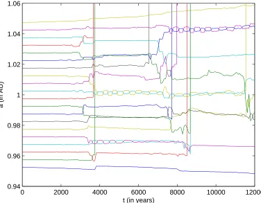
bodies is centered at 1 AU. We simulate 1000 systems, each beginning with different randomly chosen orbital phases. Figure 3.3 shows the evolution of the semimajor axis of the protoplanets in one of the simulations as a function of time; other simulations behave similarly.

increased by roughly a factor of 2.3, meaning that the spacing in units of Hill radii has decreased by a factor of 1.3. We would expect the chaotic reconfiguration to restore the typical spacing to about 5RH by reducing the number of oligarchic zones. The figure, in fact, shows 13 zones after

the first reconfiguration, compared to 20 before. Three protoplanets have collided and four have formed co-orbital groups of N = 2. The co-orbital pairs are visibly tightened over the timescale predicted by equation 3.7, which for the parameters of this simulation is about ∆t≈3×103 _years.

The configuration is then stable until the growth of the bodies again lowers their separation into the strong-scattering regime at a time of 1.1×104 _years.

The other realizations of this simulation show similar results. We find an average co-orbital population ofhNi= 1.2 in the middle of the annulus after the first reconfiguration. This value is lower than that found in Section 3.2 because the protoplanets begin to strongly scatter each other when they are just closer than the stable spacing. Only a few protoplanets can collide or join a co-orbital group before the disk becomes stable again. As described in the paradigm of Kokubo & Ida (1995), a realistic protoplanetary disk in the oligarchic phases experiences many such epochs of instability as the oligarchs grow to their final sizes.

3.4

The Equilibrium Co-Orbital Number

As the protoplanets evolve, they experience many epochs of reconfiguration that change the typical co-orbital number. The examples given in previous sections of this chapter show the result of a single reconfiguration. Our choices of initial conditions with the initial co-orbital numberhNii = 1 have resulted in a higher final co-orbital number hNif. If instead, hNii is very high, the final co-orbital number must decrease. As the disk evolves,hNiis driven to an equilibrium value where each reconfiguration leaves hNiunchanged. This value, hNieq, is the number that is physically relevant

to the protoplanetary disk.

We use a series of simulations to determinehNieqat a fixed value of Σ and σ. Each individual

simulation contains 40 co-orbital groups separated by 4RH. This spacing ensures that each

simula-tion experiences a chaotic reconfigurasimula-tion. The number of oligarchs in each group is chosen randomly to achieve the desiredhNii. All oligarchs begin with e=eH andi=iH to avoid the maximal

col-lision rate that occurs if e < α1/2_e

H (Goldreich et al., 2004b). The initial orbital phase, longitude

of periapse, and line of nodes are chosen randomly. We set a lower limit to the allowed inclination to prevent it from being damped to unreasonably small values. The results of the simulations are insensitive to the value of this limit if it is smaller thaniH; we choose 10−3iH.

1

1.5

2

2.5

3

3.5

4

1

1.5

2

2.5

3

3.5

<N>

f

<N>

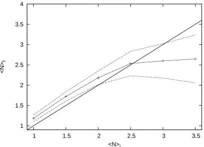
Figure 3.4 FinalhNiof simulations against the initialhNifor Σ = 0.9 g cm−2_{andσ= 9.1 g cm}−2_.

For each value of hNii the mass of each protoplanet is adjusted to keep Σ constant. The dashed lines denote the average value plus and minus one standard deviation of the measurements. The solid