Computational studies of the structure and dynamics of packings of grain and bubbles

LEABHARLANN CHOLAISTE NA TRIONOIDE, BAILE ATHA CLIATH TRINITY COLLEGE LIBRARY DUBLIN OUscoil Atha Cliath The University of Dublin

Terms and Conditions of Use of Digitised Theses from Trinity College Library Dublin

Copyright statement

All material supplied by Trinity College Library is protected by copyright (under the Copyright and Related Rights Act, 2000 as amended) and other relevant Intellectual Property Rights. By accessing and using a Digitised Thesis from Trinity College Library you acknowledge that all Intellectual Property Rights in any Works supplied are the sole and exclusive property of the copyright and/or other I PR holder. Specific copyright holders may not be explicitly identified. Use of materials from other sources within a thesis should not be construed as a claim over them.

A non-exclusive, non-transferable licence is hereby granted to those using or reproducing, in whole or in part, the material for valid purposes, providing the copyright owners are acknowledged using the normal conventions. Where specific permission to use material is required, this is identified and such permission must be sought from the copyright holder or agency cited.

Liability statement

By using a Digitised Thesis, I accept that Trinity College Dublin bears no legal responsibility for the accuracy, legality or comprehensiveness of materials contained within the thesis, and that Trinity College Dublin accepts no liability for indirect, consequential, or incidental, damages or losses arising from use of the thesis for whatever reason. Information located in a thesis may be subject to specific use constraints, details of which may not be explicitly described. It is the responsibility of potential and actual users to be aware of such constraints and to abide by them. By making use of material from a digitised thesis, you accept these copyright and disclaimer provisions. Where it is brought to the attention of Trinity College Library that there may be a breach of copyright or other restraint, it is the policy to withdraw or take down access to a thesis while the issue is being resolved.

Access Agreement

By using a Digitised Thesis from Trinity College Library you are bound by the following Terms & Conditions. Please read them carefully.

C o m p u ta tio n a l S tu d ie s o f th e S tr u c tu r e an d D y n a m ic s

o f P a ck in g s o f G rains and B u b b le s

by

Gary Delaney

A Thesis subm itted to

T he University of Dubhn

Trinity College

for the degree of

Doctor of Philosophy

SCHOOL OF PHYSICS

UNIVERSITY OF DUBLIN

TR IN ITY COLLEGE

«5^RiNlTY c o lle g e '^ 1 0 NOV

D ecla ra tio n

This thesis has not been subm itted as an exercise for a degree at any other University.

Except where otherwise stated, the work described herein has been carried out by

the author alone.

This thesis may be borrowed or copied upon request with the permission of the

Librarian, Trinity College Dublin, University of Dublin. The copyright belongs

jointly to the University of Dublin and Gary Delaney.

S u m m a r y

Since the dawn of civilization people have been intrigued by packing problems. They

have a great significance in the practicalities of our everyday lives, with people always

seeming to try to find more efficient ways of packing things together. Even though

scientists have studied them for over 2,500 years, they are still prevalent today in

almost every area of science. Much of the work th a t scientists have done on packing

problems to date has been in considering sphere packings. These have been used

widely to investigate the properties of granular materials and as simple models for

everything from packings of atoms to packings of bubbles.

We shall begin by considering one of the simplest granular systems (and indeed

one of the simplest packings of spheres) by performing the most detailed examination

to date into the physics of Newton’s Cradle. This simple system is shown to ex­

hibit many complex dynamic effects th a t give insights into the general behaviour of

granular materials and highlight how seemingly simple systems can exhibit complex

behaviour.

The them e of sphere-packing is continued when we consider bubble packings

in the wet foam limit. These packings are composed of almost spherical bubbles

th a t have been observed experimentally to dem onstrate a surprising degree of order.

We consider the similarities between these systems and computationally generated

sphere packings. We also perform two-dimensional simulations of packings of bub­

bles trapped between glass plates. The control of the position of the bubbles in

the packing is being investigated as a potential technology with applicability to the

emerging area of Discrete Microfluidics.

act under extension only. This system is seen to exhibit an onset of rigidity for

sufficient expansions th a t may in some sense be considered to be the inverse of the

onset of ‘jam m ing’ in compressed soft sphere systems.

We also go beyond traditional sphere packing models, by considering the impor­

ta n t role th a t shape plays in packings of grains. The author has created a software

program called

th a t allows for the investigation of the packing

properties of grains of arbitrary shape. The properties of random packings of ellip­

tical grains is investigated, with a very interesting variation in the packing density

of the grains observed as the ellipticity is varied.

A c k n o w le d g m e n ts

Firstly I would like express my gratitude to my supervisor, Dr. Stefan Hutzler,

whose expertise, enthusiasm, drive and support was invaluable throughout the car­

rying out of the research th at this thesis now presents. I thank Prof. Denis Weaire

for his guidance and support which added greatly to my graduate experience. I

would like to gratefully acknowledge Dr. Simon Cox for his technical assistance

w ith all things Surface Evolver and Wiebke Drenckhan and Antje van der Net for

their experimental expertise. I would also like to thank Prof. John Hinch for very

helpful discussions on Newton’s Cradle.

A big thanks goes to the enthusiastic and dedicated project students who worked

w ith me during the course of my PhD: Robert Clancy, Seamus Murphy, David Bar­

re tt and Edmond Daly.

Thank-you to all the members of our group who provided helpful discussions and

support: Eric, Vincent, Norbert, Lola, Aengus and in particular Finn MacLeod,

who wTote the original code I used to model Newton’s cradle.

A very personal thanks goes to all my friends who supported me and made Trinity

College such a great place to be: Aaron, C athal, Ciara, Colin, Denis, John, Lorna,

M artin, Orla, Rory and Siobhan.

Special thanks go to:

• Laura for the laughs, the dinners and all the things th at went with salt and

lemon!

• Barry, Eibhlin, James, Paul, Peter, Debbie, Johnny and Zillah for more great

nights than I could count.

• Clare for great nights and great holidays.

• Laina for being a brilliant holiday buddy.

• Gemma - my support scientist, my vice-convenor and lots lots more.

• Iain for many helpful technical and scientific conservations and for being a

great friend over many years.

Thank-you to all the members of rooms 4.03 and 2.22 for making the office a great

place to be: Aron, Berry, Ben, Michael, Paul and James.

I would like to acknowledge com putational support from IITAC, the Trinity Center

for High Performance Computing and the Irish Center for High End Computing.

Financial support for this PhD was provided by Enterprise Ireland Research G rant

SC/2002/0011 and a Trinity College Postgraduate Award.

Many thanks to Sonya for being everything anyone could wish for in a Sister and to

Andrew for making her so happy.

And finally to my parents, who supported me in so many ways throughout my

education and to whom I dedicate this thesis.

P u b lic a tio n s

G. Delaney, D. Weaire and S. Hutzler. Onset of rigidity for stretched string net­

works,

Europhysics Letters, 72, 990-996, 2005.

W. Drenckhan; S.J. Cox, G. Delaney, H. Holste; D. Weaire and N. Kern. Rhe-

ology of ordered foams on the way to Discrete Microfluidics,

Colloids A nd Surfaces

A-Physicochemical And Engineering Aspects, 263 52-64, 2005.

G. Delaney, D. Weaire, S. Hutzler and S. Murphy. Random packing of elliptical

disks.

Philosophical Magazine Letters, 85 2005, 89-96, 2005.

S. Hutzler, G. Delaney, D. Weaire and F. MacLeod. Rocking Newton’s cradle.

Am erican Journal O f Physics, 72 2004, 1508-1516, 2004.

C o n ten ts

1

In tr o d u ctio n

1

1.1 The im portance of packing to us a l l ...

1

1.2 Sphere P a c k in g s...

2

1.3 The role of s h a p e ...

5

1.4 Jamm ing, constraints and contact n u m b e rs ...

6

1.5 Packing inside-out

...

7

1.6 Sequential packing m o d e l s ...

8

1.7 Bubble packings and foams

...

9

1.8 Application of Computational M ethods...10

1.9 W riting S t y l e ... 13

2

N e w to n ’s C radle

15

2.1 In tro d u c tio n ... 15

2.2 Modeling Newton’s c r a d l e ... 19

2.3 R e s u lts ... 22

2.4 Theory of a two-ball c ra d le ... 25

2.5 The effects of d is s ip a tio n ...30

2.6 E x p e rim e n ts... 34

2.7 C onclusion...39

3

R a n d o m P acking

o f E lliptical D isk s

41

viii

CONTENTS

3.1

In tro d u ctio n ... 41

3.2

Simulation of 2D packings of ellipses ... 42

3.3

Results and A n a ly s is ... 45

3.4

Conclusion... 50

4 P acking L im ited G row th

51

4.1

In tro d u ctio n ... 51

4.2

T h e o ry ... 53

4.3

Computational Im p lem en tatio n ... 56

4.4

Simulation R e s u l t s ... 57

4.4.1 The transition from straight edged to circular o b je c ts ... 60

4.4.2 The role of e llip tic ity ... 62

4.4.3 Concave objects considered ... 64

4.5

Conclusion and O u tlo o k ... 67

5 P acking-driven sh ap e ev olu tion o f grains.

71

5.1

In tro d uction ... 71

5.2

Description of the M o d e l... 74

5.3

Measures of Shape ... 76

5.4

Simulation R e s u l t s ... 77

5.4.1 Short Term Simulations ... 80

5.4.2 Long Term Simulations... 85

5.4.3 Sundry parameter v ariations... 91

5.5

Discussion and C onclusion... 94

6 T h e inverse packing problem

99

6.1

Introd u ctio n ... 99

6.2

Simulation Technique... 101

C O N T E N T S

ix

6.4 I n te r p r e ta tio n ... 106

6.5 Results for the square la ttic e ... 107

6.6 Results for the hexagonal l a ttic e ...109

6.7 C o n clu sio n ... 110

7 3D sp h ere and bubble packings

113

7.1 In tro d u c tio n ... 113

7.2 Bubbles in the Wet Foam L i m i t ... 116

7.3 Random Sphere P a c k in g ... 117

7.4 Dynamic sphere packing model ... 118

7.5 Simulation R e s u l t s ... 120

7.5.1 Formation of a surface l a y e r ...120

7.5.2 Deposition of spheres onto a triangular p a c k i n g ...122

7.5.3 Deposition of spheres onto a square p a c k i n g ... 125

7.5.4 Formation of an ordered surface l a y e r ... 127

7.6 D isc u ssio n ... 128

8 Flow o f O rdered A rrays o f B u b b les

133

8.1 In tro d u c tio n ... 133

8.2 M anipulation of ordered arrays of b u b b l e s ... 134

8.2.1 Adding/removing or replacing b u b b l e s ...135

8.2.2 Sorting of bubbles into different branches of a network . . . .1 3 5

8.2.3 Controlled neighbour switching in a U - b e n d ... 137

8.2.4 Success of traditional simulation techniques ... 138

8.3 Viscous Froth M o d e l ...139

8.3.1 Quasi-static Soap Froth ... 139

8.3.2 G rain g r o w t h ... 141

X

CONTENTS

8.3.4

The Dimensionless Viscous Froth E q u a tio n ... 143

8.3.5

C u r v a tu r e ... 143

8.3.6

Determination of Bubble P r e s s u r e s ...144

8.3.7

Velocities and D is p la c e m e n t...146

8.4

Simulation R e s u l t s ... 146

8.5

Variation of system parameters ... 151

8.5.1 Variation of the radius of the b e n d ...152

8.5.2 Variation of the width of the t u b e ...153

8.5.3 Variation of the area of the b u b b le s ... 155

8.5.4 Determining the viscous drag param eter A ...157

8.6

C onclusion... 159

9

C on clu sion and O u tlook

161

A Scalin g relation sh ip s in PL G m od els.

165

B R A P and R R A P sim ulations.

169

List o f Figures

1.1 O rder of layers in H C P packing (ABABABA) and FCC packing

(AB-C A B (AB-C A )... 3

1.2 A sim ulation of a random packing of 500 spheres w ith packing fraction $ = 0.637... 4

1.3 T he A pollonian packing... 8

1.4 T he Kelvin S tru ctu re and th e W eaire-Phelan S tru c tu re ... 9

1.5 R A P packing of pentago ns... 12

2.1 D iagram of N ew ton’s cradle... 16

2.2 T he overlap of two balls... 19

2.3 Displacem ent of th e balls as a function of tim e... 22

2.4 A detailed view of th e first three sets of collisions...23

2.5 Long-tim e behavior of th e dissipation-free N = 5 cradle...24

2.6 P lot of th e relative position X r for the N = 2 cradle as a function of tim e ...27

2.7 Collision points for the N = 2 s y s t e m ... 28

2.8 Two phase p o rtraits th a t characterize the m otion of the N = 2 cradle. 29 2.9 Energy variation in the dissipative cradle... 31

2.10 Loss of energy due to the Stokes dam ping and viscoelastic dissipation for th e N = b cradle...32

2.11 E xperim ental d a ta for N ew ton’s cradle w ith N = 2, 3, and 4 balls. . . 34

L I S T OF FIGURES

2.12 Variation of the ampUtude of ball 1 in a

= 2 cradle with time. . . . 35

2.13 Variation in amplitude of ball 1 for the

N = 3

cradle... 36

2.14 Variation in amplitude of ball 1 for the

= 4 cradle... 37

2.15 Variation in ampHtude of ball 1 for a A'’ = 2 cradle with a 1 mm gap

between the rest positions of the balls... 38

3.1 Computer simulations of dense packings of elhpses...43

3.2 Variation of packing fraction $ with 1 - A... 45

3.3 Variation of packing fraction for system without elhpse rotations. . . 46

3.4 Variation of number of contacts,

Z,

with distance from edge of disks.

47

3.5 Variation of the average contact number with aspect ratio...48

4.1 RAP and RRAP packings of triangles and squares... 54

4.2 The decay of the pore space volume for triangles, pentagons and oc­

tagons

58

4.3 Plot of

N {r),

the frequency of objects of size r, for triangles, pen­

tagons and octagons... 59

4.4 The transition from straight edged to circular objects... 60

4.5 Variation of exponents

P

and

P'

for triangle to circle transition. . . .

61

4.6 RRAP packings of e llip s e s ... 63

4.7 Variation of exponents

{3

and

P'

with elhpticity...64

4.8 Concave objects considered... 65

4.9 RAP and RRAP packings of concave o b je c ts ... 66

4.10 Variation of exponents

0

and

(3'

with the concaveness 7 of the object.

67

5.1 Flow diagram for erosion model... 74

5.2 Images of order of events in simulation... 75

L I S T O F F I G U R E S xiii 5.4 Im ages show the evolution of the shapes of the grains for a short term

sim ulation w ith A $ ' = 0.02 and A $ ' = 0 .0 3 ... 79

5.5 Variation of packing fraction w ith number of iterations for short term sim ulation... 80

5.6 Variation o f convexity ratio w ith number of iterations... 81

5.7 Variation of the standard deviation cTarea of the areas of the grains w ith number of iterations...82

5.8 Variation of the average area-perimeter ratio Ja p with number of iteration s... 83

5.9 Shape evolution of the of the grains for a long term sim ulation... 84

5.10 Variation of th e packing fraction $ w ith iteration num ber... 85

5.11 Variation o f the convexity ratio f c w ith number of iterations for a long term sim ulation... 86

5.12 Variation of the standard deviation Uarea o f the area of the grains w ith number of iterations for a term sim ulations...87

5.13 Variation of the average area-perim eter ratio Ja p of the grains w ith number of iterations for long term sim ulations...88

5.14 Im ages o f sim ulations w ith large initial range of radii... 89

5.15 Im ages o f sim ulations using elliptical grains... 90

5.16 Shape evolution of two grains during the long term sim ulation... 93

6.1 E xpansion of a triangular la ttic e ... 100

6.2 Increase in th e number of tau t strings as th e periodic box is expanded, for a triangular la ttice w ith 49152 strin gs... 102

6.3 Average coordination number for a Triangular lattice above the thresh­ old of r ig i d i t y ... 103

L IS T OF FIG U RES

6.5

Variation of the average coordination number

Zcrit

at the threshold

of rigidity... 105

6.6

Disregarding vertices with coordination

z < 2

... 106

6.7

Expansion of a square lattice... 108

6.8

Variation in the fraction of vertices with coordination numbers

= 2

to

= 6 for a square lattice...109

6.9

Expansion of a hexagonal lattice... 110

6.10 Variation of the average coordination number

Zcrit

at the threshold

of rigidity for a hexagonal lattice... I l l

7.1

Packings of bubbles in wet foam...115

7.2

Ordered terraces at the bottom of the packing of bubbles...115

7.3

Forces on spheres in the dynamics simulation... 118

7.4

Formation of the surface layer...121

7.5

Packing onto a triangular layer... 122

7.6

Vertical density variation for sphere packings onto a triangular packed

layer... 123

7.7

Ordered packings generated by sequential addition of spheres... 124

7.8

Packings generated by allowing spheres to settle on a fixed square

packed layer... 125

7.9

Vertical density variation for the sphere packing onto a fixed square

packed layer... 126

7.10 Formation of an ordered surface layer using an attractive force be­

tween the surface spheres... 127

8.1

Replacement of bubbles by controlling flow/pressure in the channels. 135

8.2

Two rows of bubbles are sorted into two narrow channels...135

L I S T O F F IG U R E S xv

8.4 D iagram showing a neighbour switching T1 process... 137

8.5 A phase shift in order of the bubbles caused by passing around a U -bend... 137

8.6 Forces acting on a film segm ent of length 1...140

8.7 Flow diagram for viscous froth sim ulation... 142

8.8 T he curvature K , a t the point where edges ei and C2 m eet...144

8.9 C om parison of the distortion of a foam stru ctu re going around a bend. 147 8.10 Case 1: T he leading 3 sided bubble is on the outside as th e bubbles enter th e b e n d ... 149

8.11 Case 2: T he leading 3 sided bubble is on th e inside as th e bubbles enter th e b e n d ... 149

8.12 Case 3: T he th ird possibility is th a t th e tu b e is already filled with bubbles, before th e bubbles s ta rt to be pushed... 149

8.13 T1 process for Case 1...150

8.14 T1 process for Case 2...151

8.15 V ariation of th e critical T1 velocity Ucrit w ith th e radius of th e tube. . 152

8.16 V ariation of th e critical T1 velocity Ucrit w ith the w idth of th e tu b e for th e case of the leading outer bubble (case 1)...154

8.17 V ariation of th e critical T1 velocity Vcnt w ith th e w idth of th e tu b e for th e case of th e leading inner bubble (case 2 )... 154

8.18 V ariation of th e critical T1 velocity Ucrit w ith th e area of th e bubbles for case 1... 156

8.19 V ariation of th e critical T1 velocity Ucrit w ith th e area of th e bubbles for case 2 ... 156

8.20 T he shortest edge length L as a function of foam flow velocity v around th e U -bend...158

xvi L IS T O F F IG U R E S

B .l Variation o f exponents a and a' for triangle to circle transition. . . . 169 B .2 Variation of exponents a and a' w ith ellipticity... 170

B.3 Variation of exponents a and a' w ith the concaveness 7 o f the object. 170

C h ap ter 1

In tro d u ctio n

1.1

T h e im p o r ta n c e o f p ack in g to us all

The problem of how objects pack together has been of interest to scientists for

millennia [8]. Indeed Bernal remarked th at the problem of packing objects into a

container is one of the oldest problems known to man [12], It can be of im portance

in all our daily lives, from when we try to squeeze those last souvenirs into our suit

cases to times when we ponder upon how the bees know how to pack their honey

cells together [97].

Packing problems are still prevalent today in almost every area of science. Physi­

cists investigate with how things fit together in nature. M athem aticians concern

themselves with the theoretical aspects of packing, expending great energy at times

attem pting to prove what type of packing is best in a given situation [47]. Chemists

have historically had great success in taking a Newtonian view and considering how

atom s pack together, relating this structure to the observed physical and chemical

properties of substances [8]. Biologists even consider the geometrical contribution to

the structure of living things, for example considering the cellular packing structures

of biological cells [100, 40].

2

C H A P T E R 1. IN T R O D U C TIO N

We are surrounded in our everyday lives by granular packings, from the grains

of sand on the beach to the box of cereal th a t sits on the breakfast table [56]. They

play an im portant role in a great number of our industries, including construction,

mining and pharmaceuticals [26]. They also have great im portance in geological

processes which can have a great impact on all our lives. The study of granular

packings gives great insights into the physical mechanisms of landslides, erosion and

even plate tectonics, where the dense packing of the E a rth ’s plates is considered [55].

1.2

Sphere Packings

Often in the packing problems found in nature, as in life, the goal is maximum

density. Indeed, the dense packing of hard objects is a recurrent paradigm in physics,

from early models of crystallinity to modern theories of granular materials which

are under active debate today [8, 66]. Generally speaking the objects are taken to

be spheres in three-dimensions (or circular disks in two dimensions), leading to the

formulation of the Kepler Problem:what is their densest packing?. W hen considering

questions of the density of packings we refer to the packing fraction $ . For a 2D

packing of circles, this is simply the area covered by the circles divided by the total

area, while in the 3D case of spheres, it is the volume of the spheres divided by the

total volume.

1.2. SPHER E P A CKIN G S

3

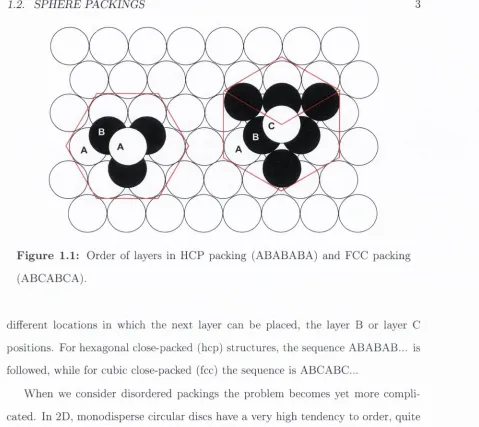
F igu re 1.1:

Order of layers in HCP packing (ABABABA) and FCC packing

(ABCABCA).

different locations in which the next layer can be placed, the layer B or layer C

positions. For hexagonal close-packed (hep) structures, the sequence ABABAB... is

followed, while for cubic close-packed (fee) the sequence is ABCABC...

W hen we consider disordered packings the problem becomes yet more compli­

cated. In 2D, monodisperse circular discs have a very high tendency to order, quite

easily finding the triangular structure. However if a small amount of polydispersity

is introduced, then the resulting packing will show a high degree of disorder, and in

general for a dense packing only achieve the random close packing of circles value of

$ « 0 . 8 4 [75, 7].

4

C H A P T E R 1. IN TR O D U C T IO N

F ig u r e 1.2: A simulation of a random packing of 500 spheres with packing

fraction $ = 0.637.

in dense packings prepared by one procedure to another (See Figure 1.2) [88, 12].

While significant, this variation is small compared to the difference between random

and ordered packings.

1.3. TH E R O L E OF SH APE

5

packing process. If the container is shaken while we pour the spheres into it, the

shaking helps to optimise the packing and a packing fraction of $ ~ 0.64 can be

achieved. However, when spheres are gently rolled into a stationary container a

packing fraction of $ ~ 0.60 is obtained. While attem pts at measuring the loosest

random packing (LRP) of spheres using neutrally buoyant spheres in liquid have

found a value of $ « 0.56 [84].

Recently new insights into the structure of random sphere packings have been

made using X-ray computed tomography of packings of up to 150,000 mono-sized

spheres with packing densities ranging from 0.58 to 0.64 [6, 5, 4]. These studies

have among other things shown th a t disordered sphere packings can be locally more

efficient th an the fee and hep crystal packings, yet more evidence of the large number

of interesting effects th a t can be seen in sphere packings.

1 .3

T h e r o le o f s h a p e

C om putational studies of random packing of particles have focused on the simulation

of sphere packings. This is the natural choice, as spheres allow a single simple

calculation to determine when two grains are in contact. However, most granular

m aterials do not consist of exactly spherical particles, and their shapes must play

a role in their properties - even the most basic property, namely density [29, 33].

Little has been done on such cases, because it is computationally demanding to

deal with the conditions of contact of irregular bodies. We utilise an approach

th a t discritises the edges of the objects, allowing us to consider random packings

of objects of arbitrary shape. In Chapter 3, we consider dense random packings of

ellipses, investigating the transition in the packing properties as the shape transitions

from circular to highly elliptical.

6

C H A P T E R 1. IN TR O D U C TIO N

in nature changes over time. This is due both to the interactions of the grains

with one another and interactions with their surroundings. We could for example

consider beach pebbles, which are subject to erosion from both their interactions

with the sea and with each other [67, 38]. In Chapter 5 we will consider a model in

which the shape of randomly packed two-dimensional grains are allowed to evolve

based on how the grains themselves pack together. This model consists of successive

generation of dense random packings of grains and the removal of small amount of

each of grain where it contacts with its neighbouring grains. It is thus the structure

of the packing of the grains itself which determines the shape evolution of the grains.

Full details of the implementation of this model are given in C hapter 5.

1.4

J a m m in g , c o n stra in ts and c o n ta c t n u m b ers

For a given configuration of particles, there exists a threshold packing fraction <I>c

at which jam ming occurs, where the particles can no longer avoid each other and

the bulk and shear moduli simultaneously become nonzero [79, 81] A ttem pts have

been made to give a strict definition of jamming, based on three hierarchical jam ­

ming categories th a t range from “locally jam m ed” , where each particle is trapped

by its neighbours, to “collectively jam m ed” where no subset of particles can simul­

taneously be displaced so th a t its members move out of contact with all particles,

to “strictly jam m ed” where no globally uniform volume-nonincreasing deformation

of the system boundary is possible [96, 36]. A recent analysis of com putationally

generated packings of particles found th a t random sphere packings with $

0.64

and random bi-disperse disk packings with $ « 0.84 were for practical purposes

strictly jam m ed [36].

1.5. P A C K I N G I N S I D E -O U T 7

been based on the concept of jamming. They consider th a t to constrain the system,

two contacts per degree of freedom are required. Thus for a random packing of

circles with two degrees of freedom (the two coordinates describing the position of

the circle) one would expect a mean contact number of 4. While for a an asymmetric

object in 2-d one would expect a mean contact number of 6 (the extra degree of

freedom being given by the angle describing the object’s orientation). These simple

argum ents th a t equate the number of contacts an object makes with its available

degrees of freedom infer a discontinuous jum p in contact number with the addition

of an infinitesimal degree of asymmetry. This is in contrast to the smooth transition

th a t we observer when we consider the transition from circles to highly elliptical

objects in C hapter 3.

1.5

P a c k in g in sid e-o u t

8

F ig u re 1.3: The Apollonian packing. This packing is formed by filling the

space between three mutually touching discs by placing a disc so th a t it just

touches the other three. The procedure is then continually repeated, filling the

new gaps generated by the addition of each new disc.

1.6

S eq u en tia l p ack in g m o d els

1.7. B UBBLE PA C K IN G S A N D FOAMS

9

F ig u re 1.4:

In

1887,

Lord Kelvin posed the problem of how to pack cells of equal

volume such th a t the to tal area of the interfaces between the cells is a minimum.

His solution, the Kelvin Strcture (Left), stood for over a century until in

1993

the W eaire-Phelan structure (Right) was discovered, beating Kelvin’s partition

by

0.3%

in area

[106].

(Images generated using the Surface Evolver).

with discretised edges, we will consider the behavior of the RAP model for objects

with various shapes in Chapter 4. We will also define a new model in which the

objects are allowed to rotate during the packing process. We will term this new

model R otational Random Apollonian Packing (RRAP).

1 .7

B u b b le p a ck in gs and foam s

10

C H A P T E R 1. IN T R O D U C TIO N

bubbles are highly disordered, except for where the packings are generated in vessels

or channels of small dimension, with only a very low number of bubbles spanning

the diam eter of the channel [54].

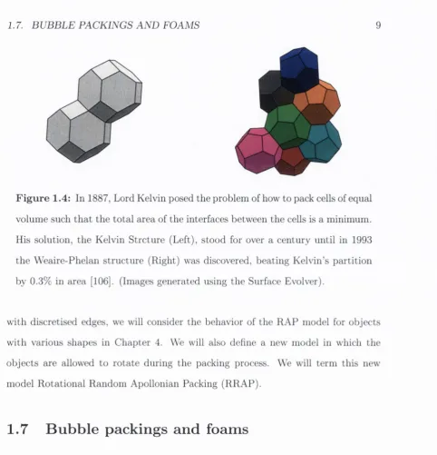
The behaviour of these foam systems are closely linked to the problem posed by

Lord Kelvin in 1887, th a t of how to pack cells of equal volume such th a t the total

area of the interfaces between the cells is a minimum (See Figure 1.6). His solution,

the Kelvin Structure, stood for over a century and is indeed observed in confined

dry monodisperse foams [54]. However in 1993 the Weaire-Phelan structure was

discovered, beating Kelvin’s partition by 0.3% in area [106]. This structure is not

observed in foam systems.

The effect of gravity driven drainage is greatly reduced as the size of the bubbles

is decreased. This allows one, when using sufficiently small bubbles, to generate a

very wet foam composed of spherical bubbles, a system with a very strong analogy

to the classically considered systems of sphere packings. When such packings of

bubbles are created they show a very large degree of ordering. We will consider such

packings in Chapter 7, comparing and contrasting their behaviour with simulation

results for sphere packings.

1.8

A p p lic a tio n o f C o m p u ta tio n a l M e th o d s.

T h e S urface E volver

1.8. A P P L IC A T IO N OF CO M PU TATIO NAL METHODS.

11

this software a user is able to define the foam structure and evolve it toward a

minimal surface energy by a gradient descent method.

Surface Evolver can also be used to implement other models using its command

language. The advantage of this approach is th a t one can take advantage of Surface

Evolver’s topological book keeping (for definitions of vertices, edges, bubbles etc.)

and its implementation of a highly optimised minimisation routine. This approach

was taken by Simon Cox when implementing a dynamic model (the Viscous Froth

Model) for the evolution of 2d foams subject to viscous forces and we utiUse this

implem entation in C hapter 8.

We also make novel use of the Surface Evolver when we consider the inverse

packing problem in C hapter 6. We modified Surface Evolver’s source code to make

the Hookean spring interaction defined in the code one-sided. We were then able to

take advantage of Surface Evolver’s implementation of periodic boundary conditions,

and its built in optimised minimisation routines.

P a ck in g o f A rb itra ry S h ap es.

We have developed a software program called

th a t allows us

to consider the packing behaviour of arbitrarily shaped grains in 2D. The software

is w ritten in the C programming language with graphics generated using

OPENGL

[25]. At the core of the software is the definition of the shape of 2D objects as

polygons and the utilising of a polygon library

C LIP P O LY

[74] to determine when

objects are in contact and the degree to which their areas overlap. Details of the

various com putational models implemented in

are given in the

relevant C hapters and Appendix C gives details of the cell list technique used to

greatly increase performance for sequential packing models.

12 CH AP TER 1. IN T R O D U C T IO N

F igu re 1.5:

RAP packing of pentagons of pentagons generated using

1.9. W R I TI NG S T Y L E 13

C hapter 3 when we consider the random packing behaviour of elhpses and further

details of the implementation of the packing algorithm are given in Section 3.2.

Ar b it r a r yPa c k e r also implements both the RAP and our new RRAP model allowing us to study the role of shape in sequential packing models. Figure 1.5 shows random packings of pentagons generated using Ar b it r a r yPa c k er and the RAP model. Full details of the implementation of the RAP and RRAP model are given in Chapter 4.

Ar b i t r a r yPa c k e r

is again used in our packing-driven shape evolution of grains

model in C hapter

Here we take advantage of the ability of the program to

pack objects of any desired shape and to even vary the shape of the objects as the

simulation proceeds. Full details of the model are given in C hapter

Finally a 3D extension to

th a t can consider sphere packings

is utilised in C hapter 7. Here both a monte-carlo packing algorithm is implemented

and a fully dynamic 3D model similar to th a t used in Chapter 2 where we consider

Newton’s Cradle. Full details of the 3D implementation are given in C hapter 7.

1.9

W r itin g S ty le

14 C H A PTE R 1. IN T R O D U C T IO N

the

software used in Chapters

and

and the modifica­

tions to Surface Evolver used in C hapter 6. The numerical results in C hapter 2, I

obtained by modifying a 2D code w ritten by Finn MacLeod [53] and the implemen­

tation of the viscous froth model in Surface Evolver th a t I utilise in C hapter 8 was

implemented by Simon Cox [58].

C h ap ter 2

N e w to n ’s C radle

2.1

I n tr o d u c tio n

A line of touching spherical balls suspended from a rail by pairs of inelastic strings

is often called a Newton’s cradle (see Fig. 2.1). The spheres are arranged at rest

in w hat is referred to as a sausage packing [8]. Interestingly, it is conjectured th at

for

N < 56, such sausage packings offer the best arrangement which minimize the

volume of the smallest convex figure containing all the spheres [108, 23].

Here we will consider Newton’s cradle in the context of a 1-dimensional granular

system. The forces th a t govern the interaction of the spheres are the same as those

considered in the study of three-dimensional granular packings. However as we shall

see even this simple 1-dimensional system displays complex dynamic behaviour and

provides excellent insights into the nature of the forces involved in 3-dimensional

granular packings.

In introductory physics textbooks, Newton’s Cradle is generally introduced as

an illustration of the conservation of momentum and energy [18, 89, 78, 72, 24, 109].

W hen one ball is displaced from the other four and released, it is claimed th a t the

collisions will result in the ball at the opposite end of the line being ejected, with

16

CHAPTER 2. N E W T O N ’S CRADLE

F ig u r e 2.1: Newton’s cradle. Ball 1 on the right is released and swings down

to im pact the line of stationary balls. It is generally suggested th a t only ball 5

on the left is ejected. However, both experiments and our simulations show th at

all balls will move after the impact.

all other balls remaining stationary. As the ejected ball swings back, it will collide

w ith the line of balls. According to the common description, only the ball th a t was

released initially will be ejected, while all other balls remain stationary.

However the actual experiment reveals a slightly different scenario. Careful ob­

servation shows th a t the first collision will break up the line of balls with the effect

th a t all balls move. After further collisions all balls will eventually swing in phase,

with an ever decreasing amplitude. The observed breakup of a line of balls after the

impact of one ball was analyzed recently by Hinch and Saint-Jean. [52] We extend

their work to consider the multiple collisions th a t follow thereafter. We believe th a t

a closer examination of Newton’s cradle can enhance and extend the pedagogical

value of the original dem onstration [49, 50, 86].

2.1. IN T R O D U C T IO N

17

Wallis (known for his presentation of

as an infinite product), Christopher Wren

(m athem atician, astronomer and architect of St. Paul’s C athedral in London), and

C hristiaan Huygens (author of a book on the wave theory of light and contributions

to probability theory). Huygens pointed out th a t an explanation required both

conservation of momentum and kinetic energy. (He did not use the kinetic energy

b u t referred to a quantity proportional to mass and velocity squared.)

However, two equations are not sufficient to describe the behavior of N ewton’s

cradle as was pointed out in Ref. [49]. A characterization of Newton’s cradle con­

sisting of

N

balls requires

N

velocities, but the conservation laws only give two

equations. Herrmann and Schmalzle[49] analyzed Newton’s cradle in terms of elas­

tic forces between the contacting balls. They argued th a t a necessary condition for

consistency with the simplified textbook description is th at there be no dispersion

in the relation between frequency and wavenumber for the vibrational motion of

the chain of contacting balls. Their conclusion was based on their experiments with

gliders on an air-track, where each glider was equipped with a spring bumper. These

experiments effectively model the first set of collisions in Newton’s cradle. W hen all

gliders are in contact, the gliders may be represented as a linear chain, allowing for

the calculation of eigenfrequencies and corresponding wave numbers. Only when the

masses of the gliders and the spring constants were chosen to achieve a dispersion-

free linear relation, did the gliders behave as in the textbook description. [49, 86]

In a follow-up paper Herrmann and Seitz[50] re-examined the actual cradle ex­

perim ent and found in both the experiments and simulations th a t the first im pact of

a ball leads to a break-up of the line, contrary to the textbook description. In their

simulations they modeled the interaction between balls as points of mass

m

th a t are

connected by (Hertzian) springs. The force between two such masses is given by

F = k { y n - V n - i T , (2.1)

18

CHAPTER 2. N E W T O N ’S CRADLE

constant, and the exponent

a = 3/2. The comparison of the propagation time of a

perturbation through a Une of balls obtained from both experiments and simulations

using a range of different values of a showed that the assumption of Hertzian springs

in Eq. (2.1) is valid. From their simulations of a five-ball cradle Herrmann and Seitz

found th at after the first collision, balls 1, 2, and 3 move backward, while balls 4

and 5 move forward with ball 4 carrying about 12% of the initial momentum of the

incident ball. (We have labeled the balls in the direction from the incoming ball

(ball 1) to the ball at the opposite end of the line (ball 5).) The momentum of ball

5 after the collision is nearly as large as that of ball 1 before the collision.

Without performing further simulations Herrmann and Seitz[50] concluded that

when ejected ball 5 swings back, it would impact not on a compact line of balls

(because the line has been broken up by the first impact), but rather there should

be a sequence of independent collisions. However, in general there can be multiple

collisions, involving more than two balls in contact during the collision as we will

see in Sec. 2.2. This issue will be examined further in relation to our experimental

results discussed in Sec. 2.6.

Hinch and Saint-Jean[52] conducted an exhaustive numerical and theoretical

study of the fragmentation of a line of

N

balls by an impact. They find that some

balls at the far end detach from the line and fly off, some in the middle hardly move,

and the impacting ball rebounds backward bringing with it some of its nearby balls.

They reproduced the numerical results of Ref. [50] for the first impact, and also set

their results into a wider context. For a linear contact force law (q = 1), the number

of balls that are detached from the line is

i V d e t a c h = 1.5iVl/^ (2.2)

2.2. MODELING N E W T O N ’S CRADLE

19

in the forward direction, for

= 15 this number increases to three. However, no

power law analogous to Eq. (2.2) was established.

Despite the above studies and recent work in the engineering literature [21], there

still is a need for further work on the nature of Newton’s cradle for the following

reasons. Because gravity was not included, the discussion was hmited to the first

impact. W hat happens in subsequent collisions? If we assume a dissipation-free sys­

tem, will the motion settle down to a regular behavior or will it be chaotic? In what

way will dissipation affect the motion? We will discuss these questions by presenting

the results of theory, experiments, and simulations where gravity has explicitly been

included, together with dissipative effects due to collisions and friction. Our work

by no means exhausts the possible corrections that might be added to the model,

but it seems sufficient for the available data.

F ig u re 2.2: The overlap of two balls.

2.2

M o d elin g N e w to n ’s cradle

We define the overlap

^rn,n

between two balls

m

and

n

as

^m,n =

(2/? - r„„)+,

(2.3)

20 C H A P T E R 2. N E W T O N ’S C R A D L E

expression inside is negative, as required for th e representation of contact forces th a t can n o t be in tension. If we model th e contact forces as described in Sec. I, th e force on ball n may be w ritten as

mXn = k[^n-l,n - C,n+l]^ (2.4)

w here X n denotes th e position of ball n.

T h e intro du ction of gravity requires some discussion. A lthough Eq. (2.4) holds for a one-dim ensional line of balls where the im pact is in the sam e direction as th e line, N ew ton’s cradle is two-dim ensional. T he balls are attach ed to a fram e by an inelastic string of length L and can swing ab o u t their respective equilibrium positions (Xo,n, along arcs of circles. T his m otion causes th e collisions to becom e off- centered if the balls are a finite distance away from their equilibrium positions. O ur m odel neglects this effect. It is restricted to small angles or am plitudes |x „ —Xo,n| < < L, in order to m aintain a one-dim ensional description of the cradle.

In th e same approxim ation, gravity can be m odeled as a simple restoring force, th a t is, a harm onic spring which acts to move each ball back to its equilibrium positions Xo,„. T he g ravitatio nal spring co nstan t is given by kg = m g / L .

T h e equations of m otion for th e dissipation-free N ew ton’s cradle are thus:

mXn = k C - l , n - kC,n+l + kg{Xo,n ~ Xn), (2.5)

w here n ranges from 1 to N . M odeling contacting spheres requires a = 3 /2 (H ertz law ).[63] T he spring co nstant k m ay be w ritten in term s of m aterial co nstants as

k = VmE / [ S { l - i y %

2.2.

MODELING N E W T O N ’S CRADLE

21

The velocity Verlet algorithm determines the positions, velocities and accelera­

tions at time ^

for each of the

n

balls in the following way:

Xn{t + A t ) = Xn{t) + Xn{ t ) At + ^X„Ai ^

(2.7)

Xn[t + — ) = Xn[t) + - X n i t ) A t

(2.8)

Xn{t + A t ) = - ( — + A t ) )

m

(2.9)

Xnit + A t ) = Xn{t + + ]^Xnit + A t ) A t

(2.10)

where

is the total force on ball

n.

It is common to introduce dimensionless variables before solving the equations

of motion numerically. However, in our problem there are two time and length

scales. Although the swinging balls may best be described in terms of their period

To =

^ /

J

and string length L, individual collisions occur on a much shorter

time scale

to — { r r ?

and displacement scale

I

= { r n ^ v ^ .

Here

v

is the

velocity of the impacting ball, given by

=

A ^ fg jL .

Because Eq. (2.5) describes a conservative system, the appropriate time step Ai

for the numerical integration may be found by checking for energy conservation.

Our chosen time step of approximately 2.5 x 10“^

to

lead to a relative error in the

energy of not more than 0.005% over a time of over 10000 Tq.

22

CHAPTER 2. N E W T O N ’S CRADLE

1

p cr

0 . 2

s

Q - 0 . 8 C - 0 . 2 0)

e

0 0 . 5 1 1. 5

Tim e (Tg)

2 2 . 5

F ig u re 2.3: Displacement from their respective equilibrium positions of each

of the five balls as a function of time. Note that the first impact results in a

fragmentation of the line of balls. Contrary to textbook explanations of Newton’s

cradle, all balls are subsequently in motion. In the early stages of this dissipation-

free simulation, the largest amplitudes of motion are exhibited by balls 1 and 5.

(The displacement is plotted as a fraction of the initial amplitude of the incident

ball. Time is displayed in multiples of the period of a single ball To = 27

.)

For

kg > 0 we found that the first collision breaks up the line of balls. As the balls

move back toward their respective equilibrium positions, however, they do not return

to their individual stationary starting positions. This difference leads to a different

scenario for the second set of collisions. As time evolves, an oscillatory motion

becomes established, as we will demonstrate in Sec. 2.4 for the case of

= 2.

2.3. RESULTS

23

1 %$» of couisions ^ M t o t c oilisjoni

Mo

Mi o(coiii««nt

Wo

F ig u re 2.4: A detailed view of the first three sets of collisions reveals the sym­

metry breaking that occurs due to the break-up of the line in the first collision.

Time is displayed in multiples of

{m^

W

e

have chosen the time origin

as the moment when the incident ball passes through its equilibrium position.

The displacements are made dimensionless by dividing by the length scale

I

.

For visual clarity they are shifted by n, where the balls are labeled from 1 to 5

as in Fig. 2.1.

time 7r/2y

results in the break-up of the line with balls 4 and 5 moving forward

and balls 1, 2, and 3 rebounding. Ball 5 reaches its maximum displacement at time

As it swings back, it will no longer hit a stationary line at time

L/g.

The second set of collisions, shown in Fig. 2.4(b) is thus not anti-symmetric to the

first set (see Fig. 2.4(a)). Figure 2.4(c) displays the third set of collisions, which is

clearly different from the first set.

24

CHAPTER 2. N E W T O N ’S CRADLE

e • •

(a) (b)

tim e (c)

F ig u re 2.5: (a) The long-time behavior of the dissipation-free

N = 5 cradle is

characterized by a slow oscillation between two modes of motion. Both modes

involve the collision of one ball against a group of four. In mode II all balls move

with a similar speed, in mode I the cluster moves much slower than the single

ball, (b) Simulation results in the form of phase-portraits. (c) A sketch of the

2.4. T H E O R Y OF A TW O -B A L L C R A D LE 25

frequency oscillations between two modes of motion. In mode I the cluster of four balls moves much slower than the single ball while in mode II all balls move with a similar speed. This behavior is particularly pronounced for = 2, but also is well pronounced for = 4 and = 5 as shown in Fig. 2.5.

2 .4

T h e o r y o f a tw o -b a ll crad le

We now present an analytical treatment of the relatively simple two-ball cradle, which leads to the identification of the behavior with the phenomenon of beats. We will show that the softness of the balls leads to an oscillation of the collision points. This variation of the phase portrait in time is also seen in our simulations of the three and four ball cradles.

Even if the balls are not infinitely hard, the standard textbook description is still valid in the sense that the impacting ball comes to a complete standstill while the impacted ball moves off with the same velocity as the impacting ball. However, what is generally ignored is the fact that the impact does not take place instantaneously. During this finite interaction time, both balls have a nonzero velocity and their point of contact will move a certain distance along the direction of the impact. (For a discussion of the related case of a bullet shot into a hanging block, see Ref. [37].) The impacted ball will move away from its equilibrium position by a distance A x and will consequently swing back after the collision. From our simulations we find that A x scales as A x oc , consistent with the displacement scale introduced in Ref. [52].

The subsequent behavior, sketched in Section 2.3 , can be analyzed as follows. If we denote the positions of each ball relative to their respective equilibrium position by x \ and X2, the center of mass Xc is given by

26 C H A P T E R 2. N E W T O N ’S C R A D L E

while th e relative position X r is

X r = X\ — X2- (2-12)

For sim plicity we shall assume a harm onic force law (w ith spring co n stan t Kr), where th e subscript r signifies th a t the interaction is due to the relative positions of th e balls. T h e validity of th e argum ent will however not be restricted to this force law. T h e cradle will be seen to be equivalent to a pair of coupled oscillators th a t are coupled only when th e two balls are in contact ( Xr > 0).

Each ball is su bject to gravitation, m odeled as a spring w ith spring constant Kc = m g / L , as in Sec. 2.2. (Previously this constant was called k^, b u t we shall use Kc in th e following discussion to rem ind us th a t the spring acts on th e center of gravity of th e two balls.) T he p otential energy of each ball is given by ^ K c X ^ . The p o te n tial energy of contact is given by ^ K r X ^ for X r > 0 and is zero for X r < 0. T he n a tu ra l frequencies associated with the two spring constants for m ass m are given by — K c / m and = Krjra.

We consider th e case where ball 1 is released from X\ — —A and X2 = 0. Then initially we have

Xc = = (2.13a)

X , = - A . (2.13b)

T he center of mass m otion is th a t of a m ass 2 m acted on by external forces {F = —KcXc) only. Hence, th e m otion is simple harm onic w ith frequency fl:

Xc = —— cosfl t. (2.14)

T he dependence of the relative position X r on th e tim e as obtained from our sim u­ lation is shown in Fig. 2.6.

T h e cradle features two tim e scales, th e collision tim e, tq and th e tim e between collisions, Fq 2> tq, given by

2.4. THEORY OF A TWO-BALL CRADLE

27

< 0 . 2

0

0.2

0 . 4

0 . 6

0 . 8

1

1 . 2

2 2 . 5 3 3 . 5 4

0 0 . 5 1 1 . 5

F ig u r e 2.6:

Plot of the relative position Xr for the

N — 2 cradle as a function of

time plotted in multiples of Fq + tq (time between collisions + interaction time).

The simulation was performed with a small ratio

K r / K c

= 100 to increase the

collision time tq.

corresponding to free motion under the action of Kc with

Xr < 0.

We make the approximation th at during a collision

{Xr > 0), where the repulsive

force due to

Kr

dominates, we neglect

Kc- Then the motion is another (short) half

cycle under

Kr,

as is seen in Fig. 2.6. We find for the interaction time tq

27t

\ / 2

:

2rn =

(2.16)

\/2 u

u;

Note th a t

\/2uj is the frequency of a single ball with a doubled spring constant.

To represent the resulting motion of the balls, it is helpful to switch identities

after every collision, so th a t ball 1

ball 2 and thus

Xr ^ —Xr.

We may then

approxim ate

Xr by

7tt

Xr

= - A c o s -

.

(2.17)

Fq + To

28

C H APTER 2. N E W T O N ’S C R A D LE

- 0 . 5

0 5 0 1 0 0 1 5 0 2 0 0 2 5 0 3 0 0 3 5 0 4 0 0

Time (r^ + Tq)

F ig u r e 2.7:

For

N = 2

successive collisions take place in tu rn on the left

(circles) and on the right (triangles) of the center of the system. The numerically

determined points are well described by theory (continuous line), Eq. (2.20).

one ball (with the above role reversal implied). For

<S F

, we obtain

where

x

denotes th a t the identity switches between

x\

and

X2

after each collision.

Thus we have high-frequency oscillations with a frequency

VL

which are modulated

by the low frequency

=

We also can calculate the positions of the collisions. When they occur, we have

X r = Q

and the position of the collision is

X^-

From Eq. (2.17) we obtain

where

U

is the time of the ith collision. Hence the corresponding position is given

—

A

cos --- —

nt

A

irt

A

-Kt

2.4. TH EO RY OF A TW O-BALL CRADLE

29

BaJI I Ball 2

■I -0.5 0

x„/A

0.5 ■I ■0.5 0 0.5

F ig u re 2.8: Two phase portraits that characterize the motion of the

N = 2

cradle. The system slowly oscillates between the case where both balls move

with the same speed and the case where one ball collides with a stationary ball.

The axes are made dimensionless by dividing the velocity of each ball by the

maximum velocity of the incoming ball and the position by the initial amplitude.

where we have used the definition of Xc in Eq. (2.11) and the approximation F »

t q .

Figure 2.7 shows the excellent agreement between the analytical expression in

Eq. (2.20) and our simulation.

The oscillation of the collision points for

= 2 is caused by the finite elastic

response of the balls. Plotting phase portraits at difi'erent times, as shown in Fig. 2.8,

reveals the same characteristics we had obtained for the

N = 5.

by

( ^ ( z + ^)(Fo + ro))

30

CHAPTER 2. N E W T O N ’S CRADLE

2.5

T h e effects o f d issip a tio n

Although the study of a dissipation-free version of Newton’s cradle is interesting in

its own right, any realistic simulation of the experiment needs to include dissipation.

Two obvious such mechanisms are the velocity-dependent viscous drag of air and

the viscoelastic dissipation associated with the collisions of the balls. We chose a

simple linear dependence on the velocity

= rjv

(Stokes law).

The inelastic character of the collisions is modeled by including a viscoelastic

dissipation force of the form [110]

into the equation of motion. Here ^ is the overlap between two balls as defined in

Eq. (2.3) and /? = 3/2 (Hertz-Kuwabara-Kono model).[110]

The equation of motion for the dissipative Newton’s cradle is then given by

The Stokes term continually removes energy from the system, while viscoelastic

dissipation occurs only during collisions. Due to the velocity dependent forces in

the system we utilize the Euler-Richardson method to solve our new equation of

motion (Eq.2.22) [102], The Euler Richardson method determines the positions,

velocities and accelerations at time ^

for each of the

n

balls in the following

way:

(2.2 1)

= X n { t ) + ^ X n { t ) A t

(2.23)

(2.24)

2.5. TH E EF F E C T S OF DISSIPATION

31

r

c

0)

(U

u

c

tfl

0 .

0 . 1

8

4

0

0 1 2 3 4 6 7

T im e (Tq)

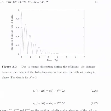
F ig u r e 2.9:

Due to energy dissipation during the colhsions, the distance

between the centers of the balls decreases in time and the balls will swing in

phase. The d a ta is for A'' = 2.

X,

,{t + At) = x{t) +

(2.26)

Xn{t + At)

=

x{t) + x ’^ '^ A t

(2.27)

where

and

are the position, velocity and acceleration of the ball

n at

the half way point of the time step

At.

We use the same tim e step as for our dissipation free simulations. The time step

was tested using the Euler-Richardson m ethod for the dissipation-free case and seen

again to give excellent energy conservation.

To dem onstrate the effect of the viscoelastic dissipation on the behavior of the

system, simulations were run where the Stokes term was neglected

= 0). In

Fig. 2.9 we plot the distance between the two balls as a function of time. This

32

C H A P TE R 2. N E W T O N ’S C R A D LE

1

0 . 9

0 1

(B •H 0 . 6

0 . 4

Dl

0 . 2

0.1

0 1 2 3

Time (Tq)

4 5 6