Preprint typeset in JHEP style - HYPER VERSION ITP-UU-11-08 SPIN-11-06 TCDMATH 11-04 HMI-11-03
Comments on the Mirror TBA
Gleb Arutyunova∗† and Sergey Frolovb†
a Institute for Theoretical Physics and Spinoza Institute,
Utrecht University, 3508 TD Utrecht, The Netherlands
b Hamilton Mathematics Institute and School of Mathematics,
Trinity College, Dublin 2, Ireland
Abstract: We discuss various aspects of excited state TBA equations describing the energy spectrum of the AdS5×S5 strings and, via the AdS/CFT correspondence, the spectrum of scaling dimensions of N = 4 SYM local operators. We observe that auxiliary roots which are used to partially enumerate solutions of the Bethe-Yang equations do not play any role in engineering excited state TBA equations via the contour deformation trick. We further argue that the TBA equations are in fact written not for a particular string state but for the whole superconformal multiplet, and, therefore, the psu(2,2|4) invariance is built in into the TBA construction.
∗Email: [email protected], [email protected]
†Correspondent fellow at Steklov Mathematical Institute, Moscow.
Contents
1. Introduction and Summary 1
2. TBA equations and asymptotic solution 4
3. Implementation of the PSU(2,2|4) symmetry 11
4. Appendix 17
4.1 Simplified TBA equations and Y-system 17
4.2 Duality transformation and transfer matrices 19
1. Introduction and Summary
The mirror Thermodynamic Bethe Ansatz (TBA) approach is the only tool currently available to determine exact energies of AdS5 ×S5 string states and, thanks to the AdS/CFT conjecture [1], scaling dimensions of N = 4 SYM local gauge-invariant composite operators. In essence, the TBA is a set of coupled non-linear integral equations for the so-called Y-functions, whose solutions are expected to yield the spectrum of the corresponding string/gauge theory.
Although the TBA approach1 has been successfully used in the case of two-dimensional relativistic integrable models for quite some time [2], its application to the AdS5×S5 superstring2 is not straightforward and requires a careful thought. Im-portantly, the string sigma model is not Lorentz invariant on the two-dimensional world-sheet and, therefore, under the double Wick rotation, which is in the heart of the TBA construction, it transforms into another model, termed in [8] a mirror. The ground state energy of the original string model is then related to the free energy (or Witten’s index, depending on the boundary conditions for fermions) of its mirror. In turn, the free energy and the TBA equations for the ground state is derivable from the so-called string hypothesis [9], which for the AdS5 ×S5 mirror model has been formulated in [10]. In this way the ground state TBA equations were obtained [11 ]-[14],3 and in [16] it was shown that the corresponding solution correctly reproduces
1We will not describe it here, referring the interested reader to the original literature [2, 3] and
recent reviews [4,5,6].
2There is currently much evidence in favor of integrability of the AdS
5×S5superstring andN = 4
SYM, see the recent collection of reviews [7] and references therein.
the vanishing energy of the ground state that corresponds to the protected half-BPS operator of the gauge theory.
The importance of the ground state TBA equations lies in the fact that they admit a generalization to excited states by means of a contour deformation trick which is similar to the analytic continuation procedure of [17], see also [18]. The contour deformation relies on an assumption that the set of TBA equations is universal for any state of the model; excited states TBA equations may differ from each other only by a choice of integration contours of convolution terms, and by analytic properties of Y-functions which determine driving terms in the TBA equations once the integration contours are taken back to the real line of the mirror model. TBA equations for string excited states in the sl(2) sector have been studied along these lines in [19]-[23]. In general, Y-functions have quite intricate analytic properties which are currently under investigation [21], [24]-[26].
In this paper we continue studies of the mirror TBA approach and make three new observations.
The first observation is on the origin of the large J asymptotic solution. As was emphasized in [27], in the largeJ or smallg limit4, the leading exponential correction to energies of string states should be given by a proper generalization of L¨uscher’s formula [28]. Such a generalization to the case of non-Lorentz invariant string sigma model and to string states containing many particles was proposed in [29] and used there to compute the four-loop anomalous dimension of the Konishi operator5. The corresponding energy correction is given in terms of YQ-functions that are in turn
expressed via transfer matrices TQ,1(v), see eq.(2.1). These transfer matrices are
associated with a scattering matrix which scatters a mirror theory Q-particle bound state of rapidity v with string theory fundamental particles. In what follows we refer to eq.(2.1) as to the Bajnok-Janik formula. We further recall that L¨uscher’s formulae provide an approximation to the exact TBA equations when YQ-functions are small.
Indeed, recently a perfect agreement has been found between L¨uscher’s formulae at five loops [33, 34] and the corresponding predictions of the mirror TBA [35,36].
In addition to the mainYQ-functions, the TBA equations also involve Y±-,YM|vw
-andYM|w-functions, as implied by the string hypothesis [11]. Thus, to know the whole
asymptotic solution, one has to also find the asymptotic expressions forY±,YM|vw and
YM|w. In this paper we show that the corresponding expressions immediately follow
from the Bajnok-Janik formula and the Y-system. We recall that the Y-system is a set of functional relations between Y-functions which is obtained from the ground
4Here J is a charge of a string state andg is the string tension which is related to the ’t Hooft
couplingλas λ= 4π2g2.
5In the context of the string sigma model L¨uscher’s approach received recently a considerable
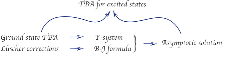
Ground state TBA Y-system Asymptotic solution B-J formula
TBA for excited states
[image:4.595.123.488.73.168.2]}
Luscher corrections..
Figure 1: The ground state TBA equations imply the Y-system. The Bajnok-Janik formula together with the Y-system leads to determination of the whole asymptotic solution. The ground state TBA equations together with the asymptotic solution allow one to engineer excited states TBA equations via the contour deformation trick.
state TBA equations by applying a certain projection operation [37]. In the context of the string sigma model the corresponding Y-system and the asymptotic solution were conjectured in [38]. The emphasis of our consideration here is on the fact that the asymptotic solution is derivable in a straightforward manner from the Y-system and the Bajnok-Janik formula, see Figure 1. In particular, in the process of the derivation, the Bazhanov-Reshetikhin formula [39] and Hirota equations [40] relating various transfer matrices emerge naturally.
Our second observation concerns the construction of excited TBA equations be-yond the sl(2) sector. As was mentioned above, obtaining excited state TBA equa-tions requires the detailed knowledge of the asymptotic solution. For generic states, the asymptotic solution is constructed in terms of transfer matrices that in addition to physical momentap1, . . . , pN of string theory particles also involve auxiliary variables
(roots) which satisfy the so-called auxiliary Bethe equations. We argue that for J
finite, a physical state is completely characterized by a set of charges it carries under the global symmetry group and by a set of momenta p1, . . . , pN; auxiliary roots, as
well as their Bethe equations, are invisible in the mirror TBA approach. Our arguing is based on the fact that all the transfer matrices and, therefore, the asymptotic Y-functions do not exhibit any singular behavior at locations of auxiliary Bethe roots. These roots satisfy auxiliary Bethe equations which guarantee regularity of transfer matrices. As a matter of fact, it is the main rational behind theanalyticBethe ansatz [4] that Bethe equations are derivable from the requirement of analyticity of the cor-responding transfer matrices. Of course, the presence of auxiliary Bethe roots affects analytic properties of Y-functions, but only in an indirect way. More precisely, as a first step towards constructing excited states TBA equations, auxiliary roots corre-sponding to a given asymptotic state must be solved in terms of physical momenta and substituted into asymptotic Y-functions, so the later become functions of p1, . . . , pN
to determine their analytic properties as functions of v and use them to engineer ex-act TBA equations via the contour deformation trick. We also point out, that the main (asymptotic) Bethe equation for some pk implies the condition Y1o∗(pk) = −1,
whereYo
1∗ is an asymptotic Y1-function analytically continued to the string theory
re-gion. For finite J these asymptotic conditions are replaced by exact Bethe equations
Y1∗(pk) = −1, where Y1∗ is an exact Y-function [18, 17]. However, there are no any
“exact equations” for determining auxiliary Bethe roots, such equations are not there already for the asymptotic solution because of the above-mentioned analyticity of the asymptotic Y-functions.
Our third observation deals with the issue of the PSU(2,2|4) symmetry. This symmetry was an important ingredient for conjecturing the all-loop asymptotic Bethe ansatz [41,42] based on the psu(2|2)⊕psu(2|2)-invariant S-matrix [43]. In the present paper we argue that PSU(2,2|4) is automatically built in into the mirror TBA ap-proach, for a simple reason of being also the symmetry of the asymptotic solution. It appears that asymptotic Y-functions are merely invariant under the action of super-symmetry generators,i.e., they are the same for any member of a given superconformal multiplet. Since the asymptotic solution is used to build exact TBA equations, the latter should be associated to the whole superconformal multiplet as well. We also point out, that the relation LT BA =J + 2 between the TBA length parameter LT BA
and the charge J established in our previous work [21] has a interesting interpreta-tion – LT BA equals to the maximal J-charge in the supersymmetry multiplet under
consideration.
The paper is organized as follows. In section 2 we give a derivation of the asymp-totic solution from the Y-system and the Bajnok-Janik formula. We further explain how to engineer excited states TBA equations by means of the contour deformation trick. We also discuss the issue of auxiliary Bethe roots. In section 3 we discuss implementations of the PSU(2,2|4) symmetry in the mirror TBA approach. In two appendices we collect the ground state TBA equations and discuss in detail duality transformation for transfer matrices, whose explicit expressions in various gradings are also provided.
2. TBA equations and asymptotic solution
The mirror TBA approach is based on a bold assumption that excited states TBA equations have the universal form for any state. The TBA equations6 may differ from each other only by a choice of integration contours of convolution terms, and by an-alytic properties of Y-functions which determine driving terms in the TBA equations once the integration contours are taken back to the real line of the mirror model. The
6For reader’s convenience, the ground state TBA equations and following from them Y-system
driving terms are of the form ±logS(u∗, v) where u∗ is either a zero, pole or −1 of
a Y-function. One can check that all the driving terms appearing via the procedure are annihilated by the operator s−1: logS·s−1(u∗, v) = 0 for |v| ≤ 2, and, therefore,
Y-functions which solve the excited states TBA equations also solve the associated Y-system equations.7
Asymptotic solution
For large J the energy of a string state can be found by solving the Bethe-Yang (BY) equations and taking into account the leading L¨uscher’s exponential corrections. The BY equations depend on momenta of fundamental particles the string state is composed of (which could be complex if there are bound state particles), and on auxiliary roots. The auxiliary roots, however, are functions of the momenta, and, as a result, an N-particle string state is completely characterized by the momenta pk
or, equivalently, by the u-plane rapidity variable uk, or by the z-torus variables zk.
Moreover, the imaginary parts of the momenta are determined by their real parts, and, therefore, the number of independent parameters is equal to the number of fundamental and bound state particles the string state is made of.
Then, at largeJ the YQ-functions become exponentially small and can be written
in terms of the su(2|2) transfer matrices defined in appendix 4.2 as follows [29]
YQo(v) = ΥQ(v)TQ,−1(v)TQ,1(v), (2.1)
ΥQ(v) =
e−JEeQ(v)
QN
i=1S 1∗Q sl(2)(ui, v)
=e−JEQe (v)
N
Y
i=1
SQ1∗
sl(2)(v, ui),
wherev is the rapidity variable of the mirrorv-plane and EeQ is the energy of a mirror
Q-particle. Here S1∗Q
sl(2) denotes the sl(2)-sector S-matrix with the first and second arguments in the string and mirror regions, respectively. The AdS5×S5 string world-sheet S-matrix is a tensor product of two su(2|2)-invariant ones, and this results in the appearance of two (in general different) transfer matrices TQ,±1(v) in (2.1). The transfer matrices TQ,±1 obviously depend on uk, and the normalization of T1,±1 is chosen so that if uk solve the BY equations then Y1o∗(uk) =−1.
The asymptotic YQ-functions (2.1) together with the Y-system equations
com-pletely fix the form of all the other Y-functions in the large J limit. Indeed, we first notice that for |v|<2 the prefactors ΥQ in (2.1) satisfy the equations [14]
Υ+QΥ−Q = ΥQ−1ΥQ+1. (2.2)
Thus, for large J the Y-system equation (4.2) takes the form
T1+,−1T1−,−1 T2,−1
T1+,1T1−,1 T2,1
= 1− 1
Y−(−)
!
1− 1
Y−(+)
!
, (2.3)
and one finds the asymptotic solution for Y−-functions
Y−(±) =−T2,±1
T1,±2
, T1,±2 ≡T1+,±1T −
1,±1−T2,±1. (2.4)
In the same way eq.(4.4) allows one to get the asymptotic solution forYQ|vw-functions
YQ(±|vw) = TQ,±1TQ+2,±1
TQ+1,±2
, TQ+1,±2 ≡TQ++1,±1T
−
Q+1,±1−TQ,±1TQ+2,±1. (2.5)
Next, moving to eq.(4.7) forY−, one determines the asymptotic Y1|w-functions
Y1(|±w)(v) = T + 1,±2T
−
1,±2−T2,±2
T2,±2
= T1,±1T1,±3
T2,±2
, T1,±3 ≡
T1++,±1 1 0
T2+,±1 T1,±1 1
T3,±1 T2−,±1 T
−−
1,±1
. (2.6)
Finally, eq.(4.9) forY1|vw-functions and eqs.(4.12) and (4.13) forYQ|w-functions allow
one to find Y+ and the remaining YQ|w-functions
Y+(±)=−T2,±3T2,±1
T3,±2T1,±2
, YQ(±|w) = T1,±Q±2T1,±Q
T2,±Q±1
, (2.7)
where the transfer matricesTa,±sare expressed throughTa,±1by means of the Bazhanov-Reshetikhin formula [39]
Ta,±s(v) = det1≤i,j≤sTa+i−j,±1
v+ i
g(s+ 1−i−j)
. (2.8)
Here one assumes that Ta,±1 satisfy the conditions: T0,±1 = 1 andTa<0,±1 = 0.
It is worth mentioning that by construction the asymptotic T-functions satisfy the T-system or Hirota equations [40]
Ta,s+Ta,s− =Ta+1,sTa−1,s +Ta,s+1Ta,s−1, a >0, s6= 0, (2.9)
where Ta,0 = 1. Clearly, the functions Ta,s were constructed from Ta,1 in a purely algebraic manner, and it remains to be proven that they actually coincide with the transfer matrices corresponding to the representations (a, s) of the centrally-extended psu(2|2). In the appendix we derive independently an explicit expression forT1,s which
can be used to check numerically that it agrees with the one obtained from Ta,1 by means of (2.8).
Obviously, in the largeJ limit the negatives T-functions are decoupled from the positive s ones. For finite J one takes the exactYQ-functions to be of the form [3,4]
YQ = ΥQ
TQ,−1TQ,1
TQ−1,0TQ+1,0
where TQ,±1 reduce to the asymptotic ones and TQ,0 reduce to 1 in the large J limit.
Then one assumes that in addition to the Hirota equations (2.9) the T-functions satisfy the following equations8
Ta,+0Ta,−0 =Ta+1,0Ta−1,0 + ΥaTa,1Ta,−1, a >0, (2.11)
and expresses all the other Y-functions in terms of Ta,±1 and Ta,0, or, equivalently, in terms of T1,s. Introducing the functions
YQ,0 =YQ, Y1,−1 =− 1
Y−(−) , Y1,1 =−
1
Y−(+), Y2,−2 =−Y
(−)
+ , Y2,2 =−Y (+)
+ ,
YQ+1,−1 = 1
YQ(−|vw) , YQ+1,1 =
1
YQ(+)|vw , Y1,−Q−1 =Y
(−)
Q|w, Y1,Q+1 =Y
(+)
Q|w, (2.12)
and performing the rescaling mentioned in footnote 8, one can write the relations in the standard form [3,4]
Ya,s =
Ta,s−1Ta,s+1
Ta−1,sTa+1,s
. (2.13)
It is important to stress that the existence of T-functions Ta,±1 andTa,0 which satisfy (2.11) does not follow from anything we know about the AdS5 ×S5 superstring or
N = 4 SYM. Fortunately, this assumption plays no role in constructing excited states TBA equations via the contour deformation trick.
Engineering TBA equations for any state
In this subsection we formulate the general strategy for engineering excited state TBA equations via the contour deformation trick. It is basically the same as the one we used in [21] to analyze the states from the sl(2) sector. The main new ingredient now is that the description of a generic state by means of the BY equations requires using not only momenta carrying Bethe roots but also a number of auxiliary ones.
1. Start with the BY equations in any grading, e.g., the sl(2) or su(2) ones, and choose a charge J, a number of fundamental particles N = KI and a set of auxiliary roots numbersKII
α andKαIIIfor the state/operator under consideration.
All the other 4 charges of the state are determined by J and the auxiliary roots numbers. The canonical dimension of the primary operator or the energy of the string state at g = 0 is given by E0 = ∆0 =J +N.
Solve the BY equations and choose from many solutions the one which corre-sponds to the state of interest. This state is characterized by a definite set of
8Since Υ
g-dependent momenta, and by the set of auxiliary roots numbers KII
α and KαIII.
Auxiliary roots are completely fixed by the momenta, and play no independent role in the description of the state. In practice a solution of the BY equations can be found only numerically for small g.
2. Compute asymptotic T- and Y-functions by using the set of momenta and aux-iliary roots for the state, and find the location of zeroes and poles of 1 +Ya,s and
Ya,s functions in the mirror and string regions. The asymptotic solution can be
trusted for finite J and small g. Note that the grading of the transfer matrices should match the grading of the BY equations used.
3. Choose integration contours and engineer TBA equations for the state so that the asymptotic TBA equations obtained by dropping the terms with log(1 +YQ)
are solved by the asymptotic solution for Y-functions.
4. The exact momenta of fundamental particles are found from the exact Bethe equationsY1∗(pk) =−1 which are derived by analytically continuing the excited
state TBA equation for Y1.
Following the steps one can write down (at least in principle) excited states TBA equations for an arbitrary string state or N = 4 primary operator.
Some important comments are in order.
• There are no equations to determine the exact location of the auxiliary roots. As we discuss in the next subsection, Y-functions are regular at the locations of auxiliary roots, and do not have neither zeroes, poles or−1’s there.
• Asymptotic Y-functions have zeroes, poles or −1’s at other locations, and ex-act Y-functions have similar properties too. Exex-act locations of these zeroes, poles and −1’s are determined by analytically continuing the TBA equations for corresponding Y-functions to their (approximate) locations, and setting the Y-functions there to 0, ∞ or −1.
• Some zeroes, poles or −1’s of asymptotic Y-functions might be spurious and be absent in exact Y-functions. For example, the analysis of a state from the
su(2)-sector composed of a fundamental particle and a two-particle bound state shows [26] that auxiliary Y-functions may have some zeroes, poles or -1’s whose contributions to the TBA equations should not be included. These spurious zeroes, poles or −1’s are outside the physical strip and related to asymptotic
• The energy spectrum computed by using the asymptotic Bethe equations is very degenerate. Most of this degeneracy is however lifted as soon as the leading exponential corrections are taken into account.
As an example, let us consider the states which have KI = 4, KII
− +K+II = 2
and KIII
α = 0. There are obviously three possible y-root distributions: (i)K−II =
0, KII
+ = 2, (ii) K−II = 2, K+II = 0, (iii) K−II = 1, K+II = 1. Since KαIII = 0 all
the y-roots satisfy one and the same equation (3.2). There are two solutions,
y1 and y2, to this equation not equal to 0 or ∞. Let one of the y-roots be equal toy1, and the other toy2. The next step is to find a solution to the main Bethe equation (3.1). This equation involves all they-roots, and, therefore, the solution is the same for any of the three states. Thus, the asymptotic energies of these states are the same. The states (i) and (ii) correspond to conjugate representations and therefore have equal energies also for finite J and g. On the other hand, computing the YQ-functions for the third state one finds that
they are different from those for the first two states. Thus, already the leading exponential correction would lift the asymptotic degeneracy of the spectrum.
We conclude this discussion with a word of caution. The procedure described above has so far been tested only for states composed of fundamental particles with real momenta. If some of the momenta are complex, e.g. there are bound states, then in the large J limit some of the asymptoticYQ-functions constructed via eq.(2.1)
develop singularities on the real line of the mirror theory. Therefore, strictly speaking, eq.(2.1) does not provide a largeJ asymptotic solution of TBA equations. We believe however that for finite J and small g eq.(2.1) or its mild modification can still be used to construct TBA and exact Bethe equations. This issue is currently under investigation [26].
Auxiliary roots and T- and Y-functions
In this subsection we discuss whether the locations of auxiliary roots yk(α) and w(kα)
are encoded in any way in analytic properties of T- and Y-functions. A naive expec-tation would be that some of the auxiliary Y-functions should be equal to −1 just as Y1∗(uk) = −1 at the locations of the main Bethe roots. We will see that this is
not the case and all T- and Y-functions are regular for any value of v related to the auxiliary roots yk(α), wk(α) by the shifts of the form in/g for integer n. Regularity of transfer matrices at locations of auxiliary Bethe roots is a well-known fact, and our discussion below is given mainly to illustrate our conclusions.
It is sufficient to consider only the roots with α = + which will be denoted as yk, wk. For definiteness we discuss transfer matrices in the mirror v-plane. The
We begin the discussion with T1,1. It is written in the form, see appendix4.2
T1,1(v) =N1(v)Ω1(v), (2.14)
where the normalization factor
N1(v) =
KII
Y
i=1
yi−x−
yi−x+
q
x+
x− (2.15)
is necessary to provide a proper normalization of Y1-functions, and
Ω1(v) = 1 +
KII
Y
i=1
v−νi+gi
v−νi−gi
KI
Y
i=1
(x−−x−i)(1−x−x+i) (x+−x−
i)(1−x+x + i)
x+
x− − (2.16)
−
KI
Y
i=1
x+−x+ i
x+−x− i
r
x−i x+i ×
KIII
Y
i=1
wi−v−2ig
wi−v +
KII
Y
i=1
v−νi+gi
v−νi−i g
KIII
Y
i=1
wi−v+2ig
wi−v
is normalized so that Ω1(uk) = 1. This guarantees that the asymptotic YQ-functions
satisfy the conditionsY1∗(uk) =−1 if the main Bethe rootsuk solve the BY equations.
Sinceνk=yk+ 1/yk, potential singularities ofT1,1 may occur either atv =νk±gi
or at v =wk. One can readily show thatT1,1 is regular atv =wk due to the auxiliary
equations for the roots wk. As to v = νk± gi, there are two cases yk = x(νk) and
yk= 1/x(νk) to be discussed. In the first case one can easily see that a potential pole
atv =νk+gi cancels out due to the normalization factorN1, andT1,1(v) is regular at
v =νk+ gi. Then, one can check that the potential pole in the normalization factor
at v =νk− gi cancels out due to the auxiliary Bethe equations for νk. In the second
case the normalization factor is regular for any v but there still exists a potential pole at v = νk + gi. A careful analysis of the residue of T1,1 at v = νk+ gi shows
that it vanishes due to the auxiliary Bethe equations for νk, and, therefore T1,1 is regular atv =νk+gi. One can also show in a similar way that 1/T1,1 is regular at all these points. Thus, both T1,1 and 1/T1,1 are regular for any value of v related to the auxiliary roots yk, wk. The same consideration shows that any asymptotic transfer
matrixTa,1 and its inverse are also regular. Since Ta,s are expressed viaTa,1 by means of the BR formula, we conclude that any Ta,s is regular for any value ofv related to
the auxiliary roots yk, wk. One can also check that 1/Ta,s is regular for these values
of v.
The regularity ofTa,s and 1/Ta,s immediately implies that no Y-function can have
either zero or pole or be equal to−1 at theseyk, wkrelated locations. Hence, we are to
2N y-roots if one uses thesl(2) grading. The asymptotic Y-functions are independent of the grading because as we show in appendix 4.2 the transfer matrices in the sl(2) andsu(2) grading can be obtained one from another by a duality transformation, and therefore, they are just equal on the solutions of the corresponding auxiliary Bethe equations. Thus, it would be unclear why one should have some extra equations for the auxiliary roots if one uses the su(2) grading.
To summarize, a physical state is completely characterized by a set of momenta of particles it is made of, and a set of auxiliary roots numbers KII
α and KαIII, while the
auxiliary roots are definite functions of the momenta. As a result, the eigenvalues of transfer matrices and Y-functions are also determined by the values of the momenta, and the location of the auxiliary roots is not reflected in their analytic properties.
3. Implementation of the
PSU(2
,
2
|
4)
symmetry
Here we discuss the issue of the PSU(2,2|4) symmetry in the mirror TBA approach. We start with the asymptotic Bethe Ansatz equations in the sl(2) grading [41]. The main Bethe equations have the form
1 = eiJ pk
KI
Y
l6=k
Ssl(2)(uk, ul) KII
−
Y
l=1
x−k −yl(−)
x+k −yl(−)
s
x+k x−k
KII +
Y
l=1
x−k −yl(+)
x+k −yl(+)
s
x+k
x−k . (3.1)
These equations are supplied with auxiliary Bethe equations for the roots y(α) and
w(α), α=±,
KI
Y
i=1
yk(α)−x−i
yk(α)−x+i
s
x+i x−i =
KIII α
Y
i=1
w(iα)−νk(α)− i g
wi(α)−νk(α)+gi , (3.2)
KII α
Y
i=1
w(kα)−νi(α)+gi
w(kα)−νi(α)− i g
= −
KIII α
Y
i=1
wk(α)−w(iα)+ 2gi
w(kα)−w(iα)− 2i g
. (3.3)
Here we introduced a concise notation νk(α) = yk(α) + 1
y(α)k . Solutions are therefore
characterized by the following five excitation numbers
(K−III, K−II, KI, K+II, K+III).
The number KI is a number of momentum-carrying particles, while KII
α and KαIII
give the weights of four SU(2) subgroups which represent a manifest symmetry of the string sigma model in the light-cone gauge. The SU(4) weights [q1, p, q2] and the spins [s1, s2] of the corresponding excited state are
q1 =K−II−2K−III s1 =KI−K−II
p=J −1 2(K
II
− +K+II) +K−III+K+III s2 =KI−K+II
q2 =K+II−2K+III
Instead of weights ofsu(4) one can use the weights (J1, J2, J3) of SO(6) and the relation
between the two is
J ≡J1 =
1
2(q1+ 2p+q2), J2 = 1
2(q1+q2), J3 = 1
2(q2−q1). (3.5) Now we are ready to discuss the realization of the PSU(2,2|4) symmetry on asymptotic solutions. First, we recall that this symmetry can be consistently real-ized only on physical states [41],i.e. those which satisfy the level-matching condition. As can be seen from eqs.(3.2) and (3.3), such states might have a certain number of rootsν(α)and w(α)located at infinity9. Second, the states belonging to the same mul-tiplet must have the one and the same anomalous dimension and canonical dimensions which might differ from each other by a half-integer only. For the light-cone string sigma model the dispersion relation is
E =J+
KI
X
k=1 r
1 + 4g2sin2 pk
2 . (3.6)
For g = 0 the last formula gives the canonical dimension of the corresponding gauge theory operator, while the differenceE−J−KIcorresponds to the anomalous dimen-sion. Thus, adding particles with zero momentum changes the canonical dimension, but does not influence the anomalous one and therefore should correspond to passing to a different member of a supersymmetry multiplet. Note that p= 0 corresponds to
u=∞in the standard u-plane parametrization of the momentum.
What was said above motivates the following treatment of the PSU(2,2|4) symme-try on the asymptotic solutions. We assume that every multiplet of PSU(2,2|4) has a unique regular representative among the solutions of the Bethe ansatz equations. Regularity means that all Bethe roots (~u, ~ν(α), ~w(α)) of the corresponding solution are finite. The regular representative10 is a primary state of the bosonic subgroup SU(2)×SU(2)×SU(2)×SU(2) and it carries excitation numbers KI, KII
α and KαIII.
All the other states in the multiplet are obtained by adding roots at infinity. Obvi-ously, the regular representative has a minimal number of Bethe roots.
In spite of the fact that irregular states in a supermultiplet have excitation num-bers different from the regular ones, they must be nevertheless described by the same Bethe equations as for the regular state. From the main equation (3.1), one sees that adding a particle with p = 0 does not influence this equation at all, since for this value of momentumx+/x− = 1. The situation is different fory-roots: Adding a single
y=∞ root will leave eq.(3.1) invariant only if the original chargeJ will be replaced as J → J − 1
2. Oppositely, adding a single y = 0 root requires a shift J → J + 1 2. Hence, there is a correlation between the number of irregular y-roots and the charge
J of the corresponding state. Finally, we note that adding any number of irregular
y- or w-roots does not influence the auxiliary Bethe equations for a regular physical state.
It is of interest to determine the Bethe root content and weights (Dynkin labels) of the superconformal primary state corresponding to a given regular state. The structure of a generic superconformal multiplet is such that primary states with re-spect to the conformal group are in correspondence with states which are obtained by acting on the superconformal primary with all possible combinations of 16 Poincar´e supercharges11. A superconformal primary state has obviously the lowest canonical
dimension in the multiplet. To understand the action of the Poincar´e supercharges, it is convenient to split them into two groups. We recall [45] that in the uniform light-cone gauge x+ = τ, where τ is the world-sheet time, the supercharges are nat-urally divided with respect to their dependence on the unphysical field x−: they are
eitherkinematical(independent of x−) ordynamical(dependent on x−). Kinematical
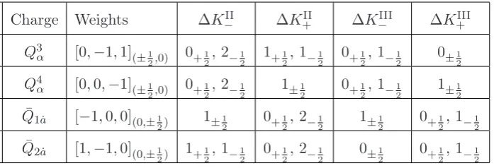
supercharges do depend on x+ and, for this reason, they do not commute with the world-sheet Hamiltonian H =E −J, while dynamical supercharges are independent of x+ and commute with H. In the Tables 1 and 2 we presented the weights of the kinematical and dynamical supercharges, respectively, as well as their action on the excitation numbers.
Charge Weights ∆K−II ∆K+II ∆K−III ∆K+III
Q3α [0,−1,1](±1
2,0) 0+ 1 2, 2−
1 2 1+
1 2, 1−
1 2 0+
1 2, 1−
1
2 0± 1 2 Q4α [0,0,−1](±1
2,0) 0+ 1 2, 2−
1
2 1± 1
2 0+ 1 2, 1−
1
2 1± 1 2 ¯
Q1 ˙a [−1,0,0](0,±12) 1±12 0+12, 2−12 1±21 0+12, 1−12 ¯
[image:14.595.124.473.382.501.2]Q2 ˙a [1,−1,0](0,±21) 1+12, 1−12 0+12, 2−12 0±12 0+12, 1−12 Table 1. Kinematical Poincar´e supercharges. These supercharges decrease J by −1/2 and increaseKI by 1, they never decrease KαII andKαIII. Here ∆KαII and ∆KαIII denote the change of the corresponding excitation numbers under the action of a supercharge.
Concerning kinematical supercharges, one can see that any such supersymmetry generator raises the number of zero momentum particles by one and, on the other hand, never lowers all the other excitation numbers. More specifically, acting with one of these supercharges adds in total either one or three irregulary-roots, depending on a supercharge under consideration. Thus, when applied to a superconformal primary state these supercharges always add further irregular roots and, therefore, can never generate the corresponding regular state.
Note that we can easily determine the location of irregulary-roots created by the action of a kinematical supercharge. Since acting with such a charge leads to the shiftJ →J−1
2, we conclude from our consideration of the main Bethe equation that
for a charge generating a single y-root the latter must be at infinity, while for one generating three y-roots, two of them must be at infinity and one at zero.
Charge Weights ∆K−II ∆K+II ∆K−III ∆K+III
Q1α [1,0,0](±1 2,0)
−1+1 2, 1−
1
2 0±
1 2
−1+1 2, 0−
1
2 0±
1 2
Q2
α [−1,1,0](±1
2,0) −1+ 1 2, 1−
1
2 0±
1
2 0+
1 2, 1−
1
2 0±
1 2
¯
Q3 ˙a [0,1,−1](0,±1
2) 0± 1
2 −1+
1 2, 1−
1
2 0±
1
2 0+
1 2, 1−
1 2
¯
Q4 ˙a [0,0,1](0,±1
2) 0±
1 2
−1+1 2, 1−
1
2 0±
1 2
−1+1 2, 0−
[image:15.595.106.488.160.277.2]1 2
Table 2. Dynamical Poincar´e supercharges. These supercharges do not change the value of KI, but they raise both J and the canonical dimension by 1/2. There exists four supercharges which lower KII by 1.
The situation with dynamical generators is a bit different. They do not change the value of KI, as they simultaneously raise E and J by 1/2. As one can see from
Table 2, there are four supercharges which have non-negative excitation numbers, and, for the same reason as for kinematical supercharges, they cannot generate a regular state from its superconformal primary. Any of the remaining four supercharges lowers
KII by one and leaves intact or lowers KIII by one. It is these generators we are most interested in, because their application to a superconformal primary state decreases the number of irregular roots and, therefore, can produce a regular state. It is also clear that we should apply all these four generators to a superconformal primary to get the regular one, as in the opposite case, there remains a possibility to further lower the number of irregular roots. Denote byEhws and Jhws the charges of a superconformal
primary, which is the highest weight state of a supersymmetry multiplet, and byEreg
and Jreg the charges of the corresponding regular state. Hence, we conclude that12
Ehws=Ereg−2, Jhws=Jreg −2. (3.7)
Also, the relationship between the corresponding excitation numbers is
KregI =KhwsI , Kα,regII =Kα,hwsII −2, Kα,regIII =Kα,hwsIII −1 (3.8) for both α. Our discussion of the main Bethe equation together with the relation
Jhws=Jreg−2 implies that four irregular y-roots which distinguish a superconformal
primary from its regular state must all be located at infinity.
12The reader can verify this formula for the case of the Konishi multiplet. We recall that the
Similar to what has been done for kinematical generators, we can now establish locations of irregular y-roots created by the action of dynamical generators. Since application of dynamical generators shifts J → J + 12, four of them generate four roots at y = 0, while the other four remove four roots at y = ∞. This leads to the following description of an arbitrary state generated by a superconformal primary
|hwsi
Y
(Qd−∞)nd∞(Qd +0)
nd 0(Qk
+∞)
nk
∞(Qk +2∞,+0)
nk
∞,0|hwsi, (3.9)
where the integers nd
∞, . . . , nk∞,0 can take any value from zero to four. Here the upper
subscript “d” or “k” in the definition of a superchargeQspecifies if it is dynamical or kinematical, respectively. The subscript of Q points the location and the number of
y-roots with + and − sign signifying if the corresponding root is added or removed, respectively. Taking into account how each supercharge increases or decreases the value ofJ, one finds that such a state has
J =Jhws+
1 2(n
d
∞+nd0−n
k
∞−nk∞,0) (3.10)
and its energy is
E =Ehws+
1 2(n
d
∞+nd0+n
k
∞+nk∞,0). (3.11)
Also, this state has the following number of main particles
KI=KregI +n∞k +nk∞,0. (3.12)
As a check, we get
E−J =Ehws − Jhws+nk∞+nk∞,0 = (3.13)
=Ereg −Jreg+n∞k +nk∞,0 =K
I reg+n
k
∞+nk∞,0 =K I,
i.e. as expected for the free dispersion relation for any member of the multiplet. Further, we see that for the state under consideration a number of irregular roots, denoted by KII, is
KII
∞ = 4−nd∞+n∞k + 2nk∞,0, (3.14)
KII
0 =n
d
0+n
k
∞,0 (3.15)
so that the total number of y-roots is KII = KII
reg +K0II+KII∞. This allows one to
express J in terms of Jreg and the number of irregulary-roots
J =Jhws+ 2 + 12(K0II− K II
∞) =Jreg+ 12(K0II− K II
∞). (3.16)
Now we turn our attention to the largeJ asymptotic solution of the mirror TBA equations. The asymptoticYQ-functions for a state of chargeJand excitation numbers
KI,KII andKIII are given by eqs.(2.1). It is important to realize that this expression
for YQ is valid not only for a regular state, but for any state in the corresponding
superconformal multiplet. As we now show, all states in a multiplet have in fact the one and same asymptotic YQ-functions. First, from the explicit expression (4.14)
for transfer matrices TQ,±1, one can see that they remain unchanged if one adds any number of infinite roots u or w(α). Second, if a state has a number of y-roots KII
0 at zero and a number ofy-roots KII
∞at infinity, then the expression for transfer matrices
shows that they are related to the transfer matrices of the corresponding regular state in a very simple fashion
TQ,+1TQ,−1 = x+
x−
12(KII∞−KII0)
TQ,reg+1TQ,reg−1. (3.17)
Accordingly, the YQ-functions of this state can be written as
YQo =x +
x−
J−Jregx+
x−
12(KII∞−KII0)
YQo,reg =YQo,reg, (3.18)
where in the last formula we used eq.(3.16). Thus, for all states in a multiplet the
YQo-functions are the same as for the regular state. Since the knowledge of YQo al-lows one to find all the other asymptotic Y-functions, we conclude that all states in a superconformal multiplet must share the one and the same asymptotic solution. Moreover, since the excited states TBA equations are engineered by using the ana-lytic properties of the asymptotic Y-functions, we conclude that these equations are constructed not for a particular state but rather for a whole supersymmetry multiplet. This implies that the PSU(2,2|4) symmetry is in some sense built in into the mirror TBA approach, in a similar way as it is for the asymptotic Bethe ansatz.
Now we point out an interesting interpretation of the TBA length parameter
LT BA. Applying all kinematical generators to a highest weight state of chargeJhws ,
in a generic situation J >3, we obtain a state of the lowest J-charge, J =Jhws−4.
Oppositely, acting on |hwsi with all dynamical generators produces a state of the highestJ-charge, J =Jhws+ 4. Thus, theJ-charge of any state in a generic multiplet
obeys inequalities
Jhws−4≤J ≤Jhws+ 4 =Jreg+ 2. (3.19)
As was found in [21], the length parameter LT BA must be related to the J-charge of
a regular state as
LT BA =Jreg + 2.
Thus, LT BA simply coincides with the maximal J-charge in a supersymmetry
One remark is in oder. A generic supersymmetry multiplet is obtained by free action of 16 Poincar´e supercharges on a highest weight state (a state of the lowest di-mension in the multiplet) and arising representations of the maximal bosonic subgroup have Dynkin labels which are obtained by adding the weights of the corresponding supercharges to Dynkin labels of the highest weight state. In the case where the re-sulting labels turn out to be negative (non-generic multiplets), special rules must be applied to find the corresponding Dynkin content13. The Konishi multiplet, which has Jhws= 0, provides an example of a non-generic multiplet; it has 216 states which are
organized in 532 representations of the maximal bosonic subgroup of the conformal group. Nevertheless, certain formulas we discussed in this section remain valid for the Konishi multiplet, for instance, the relations (3.7), and also LT BA= 4.
Acknowledgements
We are grateful to Niklas Beisert for discussions concerning superconformal symmetry. G.A. acknowledges support by the Netherlands Organization for Scientific Research (NWO) under the VICI grant 680-47-602. The work of S.F. was supported in part by the Science Foundation Ireland under Grant 09/RFP/PHY2142.
4. Appendix
4.1 Simplified TBA equations and Y-system
The simplified TBA equations for the ground state derived in [11, 14] can be written in the following form14
• Q= 1-particle
logY1(v) = log 1− 1
Y−(−)
!
1− 1
Y−(+)
!
Y2ˆ? s−log(1 +Y2)? s
− log 1− 1
Y−(−)
!
1− 1
Y+(−)
!
1− 1
Y−(+)
!
1− 1
Y+(+)
!
Y22ˆ?Kˇ ˇ? s
− log (1 +YQ)? 2 ˇKQΣ+ ˇKQ+ ˇKQ−2
ˇ
? s+ logY1?Kˇ1ˇ? s−LEˇˇ? s . (4.1)
Here and in what follows we use the definitions and conventions from [21].
It has been found [21] that for all the excited states analyzed in the TBA approach the length parameterLis related to the chargeJ carried by a string state asL=J+2.
We argue in section 3 that the relation between length and charge is universal and holds for any excited state with regular Bethe roots.
13For PSU(2,2|4) these rules can be found, for instance, in [46]. 14We set the regularization parametersh
Assuming that |v| ≤ 2 and acting on (4.1) by the operator s−1, one derives the first Y-system equation
Y1+Y1− Y2
=
1− 1
Y−(−)
1− 1
Y−(+)
1 +Y2
, (4.2)
where we use the notation f± =f(v ± i
g ∓i0) and take into account that for|v| ≤2
only the first line in (4.1) contributes.
• Q-particles
logYQ+1 = log
1 + 1
YQ(−|vw) 1 +
1
YQ(+)|vw
(1 + Y1
Q)(1 +
1
YQ+2)
? s , Q≥1. (4.3)
This equations lead to the following Y-system equations valid for any v
YQ++1YQ−+1 YQYQ+2
=
1 + 1
YQ(−|vw) 1 +
1
YQ(+)|vw
(1 +YQ) (1 +YQ+2)
. (4.4)
• y-particles, α=±
log Y (α) +
Y−(α)
(v) = log(1 +YQ)? KQy, (4.5)
logY+(α)Y−(α)(v) = 2 log
1 +Y1(|αvw)
1 +Y1(|αw) ? s (4.6)
− log (1 +YQ)? KQ+ 2 log(1 +YQ)? KxvQ1? s .
The AdS/CFT Y-system is incomplete and contains equations only forY−(α)-functions.
Their derivation is not straightforward and can be found in [11]. Assuming that Y±(α) -functions are analytic in the vicinity of the interval |v| ≤2, one gets
Y−(α)+Y
(α)−
− =
1 +Y1(|αvw)
1 +Y1(|αw)
1 1 +Y1
. (4.7)
This assumption is compatible with the kernel KQy where the cut is chosen to be for
• M|vw-strings: M ≥1 ,Y0|vw = 0
logYM(α|)vw(v) = −log(1 +YM+1)? s (4.8)
+ log(1 +YM(α−)1|vw)(1 +YM(α+1) |vw)? s+δM1log
1−Y−(α)
1−Y+(α)
ˆ
? s ,
and the Y-system equations
Y1(|αvw)+Y1(|αvw)− = 1 +Y
(α) 2|vw
1 +Y2
1−Y−(α)
1−Y+(α) (4.9)
YM(α|)+vwYM(α|vw)− =1 +YM(α−)1|vw 1 +YM(α+1) |vw 1
1 +YM+1
, M ≥2, (4.10)
• M|w-strings: M ≥1 ,Y0|w = 0
logYM(α|)w = log(1 +YM(α−)1|w)(1 +YM(α+1) |w)? s+δM1 log
1− 1
Y−(α)
1− 1
Y+(α)
ˆ
? s . (4.11)
and the Y-system equations
Y1(|αw)+Y1(|αw)− =1 +Y2(|αw)
1− 1
Y−(α)
1− 1
Y+(α)
(4.12)
YM(α|)+w YM(α|w)− =1 +YM(α−)1|w 1 +YM(α+1) |w , M ≥2, (4.13)
Let us stress again that the equations above are valid only for|v| ≤2. For other values of v one should use an analytic continuation, and the resulting equations depend on it.
4.2 Duality transformation and transfer matrices
The duality transformation of the y-roots can be implemented on the level of transfer matrices and used to obtain explicit expressions forTa,1 andT1,s in thesl(2) andsu(2)
gradings. This consideration seems to give support to the statement that auxiliary roots do not play any role for T-functions because their number and their values change under a duality transformation.
The eigenvalues of the transfer matrixTa,1 in thesl(2)-grading conjectured in [47]
were obtained in [48] by using previously found scattering matrices for string bound states. The transfer matrix Ta,1 depends on the rapidities u1, . . . , uN of N ≡ KI
Bethe equations. The Y-functions also involve the transfer matricesTa,−1, which have
the same structure as Ta,1 with the replacement (y(+), w(+)) for (y(−), w(−)). Thus,
in what follows we consider Ta,1 only and, for the sake of simplicity15, denote the
auxiliary roots as (y, w). The transfer matrix Ta,1 in the sl(2) grading reads
Ta,sl(2)1 (v) =
KII
Y
i=1
yi−x− yi−x+
q
x+
x−
1 +
KII
Y
i=1
v−νi+gia v−νi−gia
KI
Y
i=1
h(x−−x−
i)(1−x
−x+ i)
(x+−x− i)(1−x+x
+ i) x+ x− i (4.14) +
a−1 X
k=1
KII
Y
i=1
v−νi+gia v−νi+gi(a−2k)
h K
I
Y
i=1
x(v+(a−2k)gi)−x−i x(v+(a−2k)i
g)−x + i + KI Y i=1
1−x(v+(a−2k)gi)x−i
1−x(v+(a−2k)i g)x
+ i i K I Y i=1
x+−x+ i x+−x−
i
v−vi−(2k+1−a)gi v−vi+(a−1)gi
−
a−1 X
k=0
KII
Y
i=1
v−νi+gia v−νi+gi(a−2k)
KI
Y
i=1
x+−x+ i x+−x−
i
r
x−i x+i
v−vi−(2k+1−a)gi v−vi+(a−1)gi
KIII
Y
i=1
wi−v+i(2k−g1−a)
wi−v+i(2k+1g −a)
−
a−1 X
k=0
KII
Y
i=1
v−νi+gia v−νi+gi(a−2k−2)
KI
Y
i=1
x+−x+ i x+−x−
i
r
x−i x+i
v−vi−(2k+1−a)gi v−vi+(a−1)gi
KIII
Y
i=1
wi−v+gi(2k+3−a) wi−v+gi(2k+1−a)
.
In this formula
v =x++ 1
x+ − i ga=x
−
+ 1
x− + i ga .
The variablev takes values in the mirror theoryv-plane, so thatx± =x(v±i
ga) with
x(v) being the mirror theory x-function. Similarly, x±j =xs(uj ± gi), where xs is the
string theory x-function. The overall factor
Na(v) = KII
Y
i=1
yi−x− yi−x+
q
x+
x− (4.15)
satisfies N +
a N
−
a =Na−1Na+1 and is, therefore, a gauge transformation which drops
from the auxiliary Y-functions.
Concerning the structure of Ta,sl1(2), we point out that the unity occurring in the first line of (4.14) can be considered as coming from the first product (in the square brackets) in the second line with k = 0, while the second term in the first line can be considered as coming from the first product in the second line with k =a.
To discuss the duality transformation, see e.g. [49,41,47] and reference therein,16
15We will also not distinguished between a transfer matrix and its eigenvalues.
16The derivation of the dual form of the Bethe equations basically repeats the one performed in
we introduce the following polynomial in the variable y of degree17 KI+ 2KIII
P(y) =
KI
Y
i=1
(y−x−i )
s x+i x−i
KIII
Y
i=1
ywi−y−
1 y + i g − KI Y i=1
(y−x+i )
KIII
Y
i=1
ywi−y−
1 y − i g . (4.16)
This polynomial has KII roots y
i that are solutions of the Bethe equations (3.2).
Therefore, this polynomial can be written in the form
P(y) = c
KII
Y
i=1
(y−yi)
e
KII
Y
i=1
(y−y˜i). (4.17)
HereKeII=KI−KII+ 2KIII is the number of the dual roots ˜yi. Thus, the ratio
R(y) = P(y)
QKII
i=1(y−yi) QKeII
i=1(y−y˜i)
=c (4.18)
is a constant independent ofy. As a result, one hasR(a) =R(b) for any aandb, that is
KII
Y
i=1
yi−a
yi−b
= P(a)
P(b)
e
KII
Y
i=1 ˜
yi−b
˜
yi−a
. (4.19)
In particular,
R(x+) = R(x−), R(1/x+) = R(1/x−), (4.20)
yielding
KII
Y
i=1
yi−x−
yi−x+
= P(x
−)
P(x+)
e
KII
Y
i=1 ˜
yi−x+
˜
yi−x−
,
KII
Y
i=1
yi− x1−
yi− x1+
= P( 1
x−)
P(x1+)
e
KII
Y
i=1 ˜
yi− x1+
˜
yi− x1−
. (4.21)
We start with showing how the auxiliary Bethe equations (3.2) and (3.3) are dualized. By construction, ˜yk is a root of P(y),i.e. P(˜yk) = 0, which is nothing else
but the Bethe equations for ˜yk:
KI
Y
i=1 ˜
yk−x−i
˜
yk−x+i
s
x+i x−i =
KIII
Y
i=1
wi−ν˜k−gi
wi−ν˜k+gi
, (4.22)
17To simplify the derivation, we assume that the level-matching condition is not imposed. We
where k= 1, . . . ,KeII. Next, introducing x±(w)
w± i
g =x ±
(w) + 1
x±(w), (4.23)
we factorize
wk−y−
1
y ± i g = (x
±
(wk)−y)
1− 1
yx±(w
k) . (4.24) Thus, KII Y i=1
wk−νi+ gi
wk−νi− gi
=
KII
Y
i=1
(yi−x+(wk))
yi− x+(1w k)
(yi−x−(wk))
yi− x−(1w
k)
= (4.25)
=
P(x+(wk))P
1
x+(w k)
P(x−(w
k))P
1
x−(w
k) ˜ KII Y i=1
wk−ν˜i− gi
wk−ν˜i+ gi
.
Therefore, the Bethe equations (3.3) acquire the form
˜
KII
Y
i=1
wk−ν˜i+ gi
wk−ν˜i− gi
=−
P(x+(w
k))P
1
x+(w k)
P(x−(w
k))P
1
x−(w k)
KIII
Y
i=1
wk−wi−2gi
wk−wi+2gi
. (4.26)
By using eq.(4.16), it is easy to compute
P(x+(w
k))P
1
x+(w k)
P(x−(w
k))P
1
x−(w k)
=
KI
Y
i=1
(x+(w)−x+
i )
1− 1
x+ix+(w k)
(x−(w)−x−
i )
1− 1
x−i x−(w k)
KIII
Y
i=1
wk−wi+2gi
wk−wi− 2gi
!2 = = KIII Y i=1
wk−wi+2gi
wk−wi− 2gi
!2
. (4.27)
Substituting this formula into (4.26), we obtain the dualized auxiliary Bethe equations
˜
KII
Y
i=1
wk−ν˜i+ gi
wk−ν˜i− gi
=
KIII
Y
i=1
wk−wi+2gi
wk−wi− 2gi
. (4.28)
Let us now discuss the duality transformation of Ta,sl1(2). For the simplest case of
the summation indexk →k+ 1. This rearrangement yields
Ta,sl(2)1 (v) =
KII
Y
i=1
yi−x− yi−x+
q
x+
x−
1−
KI
Y
i=1
x+−x+ i x+−x−
i
r
x−i x+i
KIII
Y
i=1
wi−v−gi(a+1)
wi−v−gi(a−1) (4.29)
+
KII
Y
i=1
v−νi+iga v−νi−iga
h K
I
Y
i=1
(x−−x−
i )(1−x−x + i )
(x+−x−
i )(1−x+x + i)
x+
x− −
KI
Y
i=1
x+−x+ i x+−x−
i
r
x−i x+i
v−vi−(a−1)gi v−vi+(a−1)gi
KIII
Y
i=1
wi−v+i(ag+1) wi−v+i(ag−1)
i
+
a−1 X k=1 KII Y i=1
v−νi+gia v−νi+gi(a−2k)
h K
I
Y
i=1
x(v+(a−2k)gi)−x−i x(v+(a−2k)gi)−x+i
x+−x+i x+−x−
i
v−vi+(a−2k−1)gi v−vi+(a−1)gi +
+
KI
Y
i=1
1−x(v+(a−2k)i g)x
−
i
1−x(v+(a−2k)gi)x+i x+−x+
i x+−x−
i
v−vi+(a−2k−1)gi v−vi+(a−1)gi
−
KI
Y
i=1
x+−x+ i x+−x−
i
r
x−i x+i
v−vi+(a−2k−1)gi v−vi+(a−1)gi
KIII
Y
i=1
wi−v+i(2k−g1−a)
wi−v+i(2k+1
−a) g
−
KI
Y
i=1
x+−x+ i x+−x−
i
r
x−i x+i
v−vi+(a−2k+1)gi v−vi+(a−1)gi
KIII
Y
i=1
wi−v+i(2k+1
−a) g
wi−v+i(2k−g1−a)
i
.
By using the polynomial P defined in (4.16) and performing tedious but straightfor-ward computation, one can show that the last formula can be written in the following more compact form
Ta,sl1(2)(v) =P(x+)
KII
Y
i=1
yi−x− yi−x+
q x+ x− KI Y i=1 1
x+−x− i
r
x−i x+i
KIII
Y
i=1
1
x+(w
i−v−ig(a−1))
(4.30)
−P x1−
KII
Y
i=1
yi−x1+
yi− 1 x− q x+ x− KI Y i=1
x−−x−i
(x+−x− i )(
1 x+−x
+ i) KIII Y i=1 x− wi−v+gi(a−1)
−
a−1 X
k=1
P 1
x(v+gi(a−2k))
Px(v+ gi(a−2k))
KI
Y
i=1
1 (x+−x−
i)( 1 x+−x
+ i)
r
x−i x+i ×
×
KII
Y
i=1
(yi−x−)(yi− 1 x+)
(yi−x(v+gi(a−2k))) yi− 1 x(v+gi(a−2k))
q x+ x− KIII Y i=1
(wi −v −
i
g(a−2k+ 1))(wi−v− i
g(a−2k−1)) .
We further change ˜yi →yi, KeII→KII and denote the corresponding transfer matrix
as Ta,su1(2). It reads18
Ta,su1(2)(v) =xx+−
K I 2 KII Y i=1
yi−x+ yi−x−
q
x−
x+
P(x−)
KI
Y
i=1 1
x+−x− i
r
x−i x+i
KIII
Y
i=1
1
x−(w
i−v−gi(a−1))
−P x1+
KI
Y
i=1
x−−x−i
(x+−x− i )(
1 x+−x
+ i)
KII
Y
i=1
v−νi−gia v−νi+gia
KIII
Y
i=1
x+
wi−v+gi(a−1)
−P(x−)P 1
x+ KI Y i=1 1 (x+−x−
i ) x1+−x + i
r
x−i x+i ×
×
a−1 X
k=1
KII
Y
i=1
v−νi+gi(a−2k) v−νi+gia
KIII
Y
i=1
(wi−v−
i
g(a−2k+ 1))(wi−v− i
g(a−2k−1)) x− x+ . (4.31)
The transfer matrix above is Ta,1 in the su(2) grading. The number KII should be
understood here as a number ofy-roots which the corresponding state exhibits in the
su(2) grading.
Now we turn our attention to the transfer matrixT1,s. To obtain thesl(2) graded
version of this transfer matrix, one can apply the complex conjugation to Ta,su1(2) re-garding the roots u, y, w as real and then pick up a certain normalization factor. For real u complex conjugation transforms x+i into x−i and vice versa. This motivates us to introduce a polynomial
Pc(y) = KI
Y
i=1
(y−x+i )
s x−i x+i
KIII
Y
i=1
ywi−y−
1 y − i g − KI Y i=1
(y−x−i )
KIII
Y
i=1
ywi−y−
1 y + i g (4.32)
which is complex conjugation of P defined in eq.(4.16). Using this polynomial and
18Note that eq.(4.30) contains a factor x+ x−
12KII
. When dualizing, one should expressKII via
e
KII, which givesx+
x−
KII
=xx−+
KeII
x+
x−
12K I+KIII
replacing a→s, we obtain the following expression for the transfer matrix T1sl,s(2)
T1sl,s(2)(v) = Ms KII
Y
i=1
yi−x− yi−x+
q
x+
x−
Pc(x+) KI
Y
i=1 1
x−−x+ i
r
x+i x−i
KIII
Y
i=1
1
x+(w
i−v+gi(s−1))
−Pc x1−
KI
Y
i=1
x+−x+ i
(x−−x+ i )(
1 x−−x
−
i) KII
Y
i=1
v−νi+gis v−νi−gis
KIII
Y
i=1
x− wi−v−ig(s−1)
−Pc(x+)Pc x1−
KI
Y
i=1
1 (x−−x+
i) 1 x−−x
−
i
r
x+i x−i ×
×
s−1 X
k=1
KII
Y
i=1
v−νi−gi(s−2k) v−νi−gis
KIII
Y
i=1
(wi−v+
i
g(s−2k+ 1))(wi−v+ i
g(s−2k−1)) x+ x− . (4.33)
Here the overall normalization factor
Ms= (−1)s KI
Y
i=1 x−
i x+i
s2 x−−x+ i x+−x−
i s−1 Y
k=1
x(v+i
g(s−2k))−x + i
x(v−i
g(s−2k))−x
−
i
has been found by requiring thatT1sl,s(2)reproducesTa,sl(2)1 through Bazhanov-Reshetikhin formula. Note that Ms is also a gauge transformation.
Finally, we present for completeness the transfer matrixT1,s in the su(2) grading.
It is obtained by complex conjugation of Ta,sl1(2) and picking up a proper normalization factor :
T1su,s(2)(v) =Ms
x+ x− K I 2 KII Y i=1
yi−x+ yi−x−
q
x−
x+
Pc(x−) KI
Y
i=1 1
x−−x+ i
r
x+i x−i
KIII
Y
i=1
1
x−(w
i−v+gi(s−1))
− Pc x1+
KII
Y
i=1
v−νi−gis v−νi+gis
KI
Y
i=1
x+−x+ i
(x−−x+ i )(
1 x−−x
− i) KIII Y i=1 x+
wi−v−gi(s−1) (4.34)
−
s−1 X
k=1 Pc
1
x(v−i g(s−2k))
Pc
x(v− i
g(s−2k))
K
I
Y
i=1
1 (x−−x+
i)( 1 x−−x
−
i )
r
x+i x−i ×
×
KII
Y
i=1
v−νi−gis v−νi−ig(s−2k)
KIII
Y
i=1
(wi−v+
i
g(s−2k+ 1))(wi−v + i
g(s−2k−1)) .
References
[1] J. M. Maldacena, “The large N limit of superconformal field theories and
supergravity,” Adv. Theor. Math. Phys. 2 (1998) 231 [Int. J. Theor. Phys.38 (1999) 1113] [arXiv:hep-th/9711200].
[2] A. B. Zamolodchikov, “Thermodynamic Bethe Ansatz in Relativistic Models. Scaling Three State Potts and Lee–Yang Models,” Nucl. Phys. B342(1990) 695.
[3] A. Kuniba, T. Nakanishi and J. Suzuki, “Functional relations in solvable lattice models. 1: Functional relations and representation theory,” Int. J. Mod. Phys. A 9
(1994) 5215 [arXiv:hep-th/9309137].
[4] A. Kuniba, T. Nakanishi, J. Suzuki, “T-systems and Y-systems in integrable systems,” J. Phys. A 44(2011) 103001 [arXiv:1010.1344 [hep-th]].
[5] G. Arutyunov and S. Frolov, “Foundations of the AdS5×S5 Superstring. Part I,” J. Phys. A 42(2009) 254003 [arXiv:0901.4937 [hep-th]].
[6] Z. Bajnok, “Review of AdS/CFT Integrability, Chapter III.6: Thermodynamic Bethe Ansatz,” arXiv:1012.3995 [hep-th].
[7] N. Beisert et al., “Review of AdS/CFT Integrability: An Overview,” arXiv:1012.3982 [hep-th].
[8] G. Arutyunov and S. Frolov, “On String S-matrix, Bound States and TBA,” JHEP
0712(2007) 024, hep-th/0710.1568.
[9] M. Takahashi, “One-Dimensional Hubbard Model at Finite Temperature,” Prog. Theor. Phys. 47(1972) 69.
[10] G. Arutyunov and S. Frolov, “String hypothesis for the AdS5×S5 mirror,” JHEP
0903(2009) 152 [arXiv:0901.1417 [hep-th]].
[11] G. Arutyunov and S. Frolov, “Thermodynamic Bethe Ansatz for the AdS5×S5 Mirror Model,” JHEP 0905(2009) 068 [arXiv:0903.0141 [hep-th]].
[12] D. Bombardelli, D. Fioravanti and R. Tateo, “Thermodynamic Bethe Ansatz for planar AdS/CFT: a proposal,” J. Phys. A 42(2009) 375401 [arXiv:0902.3930].
[13] N. Gromov, V. Kazakov, A. Kozak and P. Vieira, “Exact Spectrum of Anomalous Dimensions of Planar N = 4 Supersymmetric Yang-Mills Theory: TBA and excited states,” Lett. Math. Phys.91 (2010) 265 [arXiv:0902.4458 [hep-th]].
[14] G. Arutyunov and S. Frolov, “Simplified TBA equations of the AdS5×S5 mirror model,” JHEP 0911(2009) 019 [arXiv:0907.2647 [hep-th]].

![Crystal structure of 4 {2 [4 (dimethylamino)phenyl]diazen 1 yl} 1 methylpyridinium iodide](data:image/gif;base64,R0lGODlhAQABAIAAAP///wAAACH5BAEAAAAALAAAAAABAAEAAAICRAEAOw==)