Surface effects in simple molecular systems

Thesis by Edward Jay Chapyak

In Partial Fulfillment of the Requirements For the Degree of

Doctor of Philosophy

California Institute of Technology Pas(l.dena, California

1972

ACKNOWLEDGMENTS

I wish to express my gratitude to Professor Milton Plesset, my undergraduate and thesis advisor, for his encouragement and advice during the course of this research. His assistance in both academic and non-academic matters is greatly appreciated.

I gratefully acknowledge financial assistance from the National Defense Education Act, the National Science Foundation, and the

Institute 1 _{s Graduate Teaching Assistantship program. Acknowledgment} is also due the Office of Naval Research for their support of this

investigation.

ABSTRACT

This thesis examines two problems concerned with surface effects in simple molecular systems. The first is the problem asso-ciated with the interaction of a fluid with a solid boundary, and the second originates from the interaction of a liquid with its own vapor.

For a fluid in contact with a solid wall, two sets of integro-differential equations, involving the molecular distribution functions of the system, are derived. One of these is a particular form of the well-known Bogolyubov-Born-Green-Kirkwood-Yvon equations. For the second set, the derivation,in contrast with the formulation of the B.B.G.K. Y. hierarchy, is independent of the pair-potential assump-tion. The density of the fluid, expressed as a power series in the uniform fluid density, is obtained by solving these equations under the requirement that the wall be ideal.

TABLE OF CONTENTS CHAPTER

I. GENERAL INTRODUCTION

PAGE 1

PART I: THE FLUID-SOLID INTERFACE 6 II. REVIEW AND MODIFICATION OF PREVIOUS THEORIES 7

A. Introduction 7

B. The B. B. G. K. Y. Approach

C. Modification of B. B. G. K. Y. Approach D. The Series Solution

III. FORMULATION OF A NEW APPROACH

8 8 15 24

A. Derivation of the Equations 24

B. Observations and Extensions 30

C. Series Solution Using the Pair-Potential Condition 33 PART II: THE LIQUID-VAPOR INTERFACE 41

IV. THE GENERAL LIQUID-VAPOR INTERFACE 42

A. The Thermodynamic Approach B. The Kirkwood-Buff Method

C.

Structure of the Interface D. Numerical Results

E. Summary and Conclusions

V. THE LIQUID- VAPOR SYSTEM NEAR THE CRITICAL POINT

A. Introduction

B. A Statistical Mechanical Approach

C. Temperature Dependence of the Surface Tension D. Summary and Conclusions

APPENDIX

A. Comments on Uniqueness

B. The Functional Expansion Technique REFERENCES

42 44 52 70

95

97

97

103 114 119

I. GENERAL INTRODUCTION

Whenever macroscopically dissimilar materials are in contact, the molecules or atoms of one material near the contact surface in-teract with their counterparts across the surface. These interactions may give rise to important macroscopic effects. Examples of phe-nomena where surface effects play an important role include phase transition, nucleation, gas adsorption, behavior of solid state com-ponents, fluid-gas interactions and various chemical reactions.

In this thesis we use the equilibrium statistical mechanical theory of classical fluids to investigate liquid-solid interactions (adsorption) and the surface characteristics of liquid-vapor phase transitions. Because of the technological and scientific importance of fluid-solid interactions and phase transitions, a study of these phe-nomena is certainly justified. A rigorous statistical mechanical ap-proach is employed so that the basic goal of predicting observables solely from a knowledge of intermolecular forces can be achieved.

N equations involving the various distribution functions of statistical mechanics for a classical N-particle system. Slight variations of these equations were developed independently by Bogolyubov, Born, Green, Kirkwood, and Yvon. Th e n th equation of the set involves . not only the nth_ order distribution function, but also the (n+l )th. Hence, a complete analysis of any problem would involve solving N coupled,integro-differential equations. The B. B. G. K. Y. equations are valid only if the pair-potential condition, Eq. (2. I), is satisfied.

In Chapter II we apply the B. B. G. K. Y. equations to the prob-lem of a fluid interacting with a plane wall. Although the solution to this problem has been obtained by Fisher (Ref. 3, p. I 06 ), we be -lieved it instructive to formulate the equations and the statement of the problem in a manner paralleling the development of a different set of equations, presented in Chapter III. These new equations have an advantage over those obtained from the B. B. G. K. Y. approach in that their validity is in no way limited by the assumption of pair -wise in-teractions. They are, therefore, completely general. It is also demonstrated in Chapter III that the solution of the new equations reduces to the solution of the B.B.G.K. Y. equations when the pair-wise interaction condition of Eq. (2. I) is imposed. From these solu-tions one may calculate most of the important,measurable quantities associated with the adsorption process.

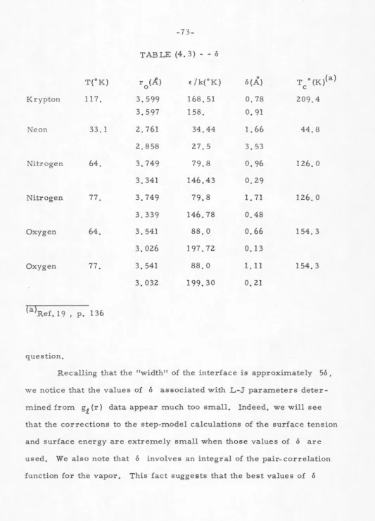
terms of the density and the second-order distribution function. Numerical results have been obtained[ 4] ' [ S] from these equations when the microstructure of the interface is ignored. In Chapter IV we include, in an approximate manner, the effect of the mic rostruc -ture and thereby improve upon these calculations.

The transition region has been analyzed by several

authors[

b] ' [

?] ' [

8 ] ' [ 9 ] ' [ lO]' [ 11 ]using methods grounded in ther-modynamical reasoning. The fact that the results predicted by such methods compare poorly with experiment (at least when the system is far from its critical point) supports the widely held opinion that

thermodynamic theories of the interface cannot accurately explain interfacial properties. It has long been recognized that a solution of the B. B. G. K. Y. equations, applied to the liquid-vapor problem,would provide the necessary information about the transition region for a system whose total potential energy can be expressed by the sum of pair-potentials. The number of these equations must, of course, be drastically reduced so that a solution can be found without reaching the limit of present computational techniques. The simplest way to achieve this reduction is to use the superposition approximation, first introduced by Kirkwood, which approximates the third order distri-bution function in terms of a product of second order distribution functions. Unfortunately, even this resulting system of two equations is nearly impossible to solve.

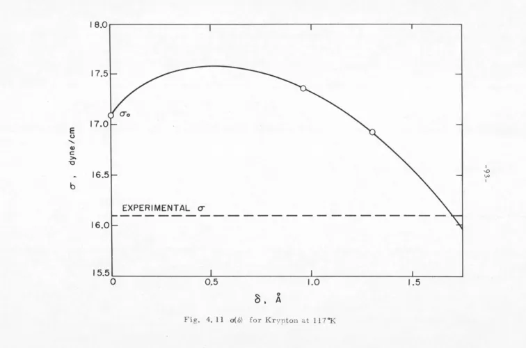
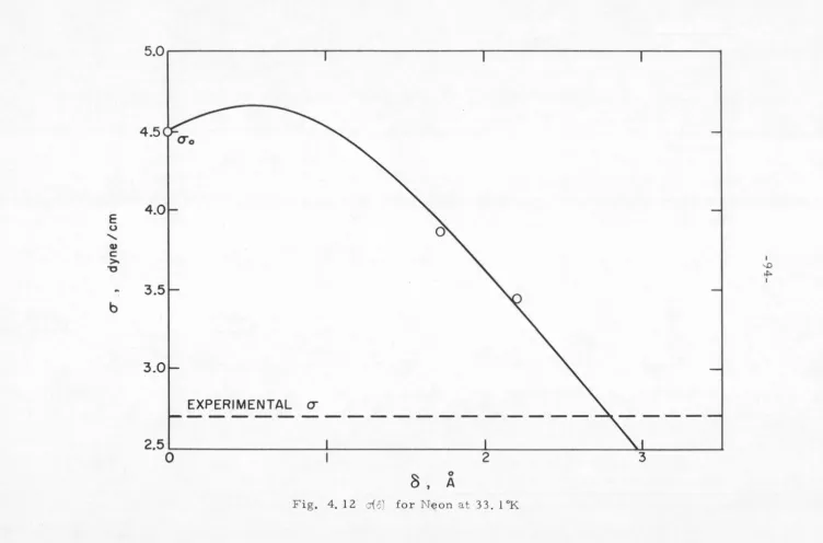
so doing, we derive a system of N equations that describes the transition region when the vapor density is much smaller than the liquid density. These equations, when simplified by the superposition approximation, can be solved easily. The resulting solutions are substituted into the expressions for the surface energy and surface tension, and numerical results are obtained for the liquidvapor sys -terns: oxygen, nitrogen, neon, and krypton.

One of the more interesting aspects of the transition region is the manner in which the density of the fluid changes as one proceeds from the vapor side to the liquid side. The theory presented in

Chapter IV predicts the existence of a length scale that characterizes the density variation through the interface. This characteristic length depends on the liquid density, temperature, and the inter -molecular potential. In particular, the length scale increases with temperature, decreases with liquid density, and decreases with in-creasing strength of the intermolecular potential. If in fact, the potential is too weak, no physical solution to the equations exists. This result suggests that a dominant factor in the formation of two phases is the existence of a sufficiently strong ,attractive intermolec -ular potential.

Finally, in Chapter V we analyze the liquid-vapor system near the critical point. Because of the fact that the transition region be-comes very broad as the critical point is approached, several

equations, modified by certain critical point assumptions, we

PART I

II. REVIEW AND MODIFICATION OF PREVIOUS THEORIES

A. INTRODUCTION

There exist various theories that attempt to describe the

interaction between a solid and a collection of fluid molecules':'. Most of these utilize the kinetic theory of gases at some stage in their

development. Thus, the actual dynamics of the molecules - - in particular the molecular flux impinging on the solid and the corre -sponding residence time of the molecules near the surface of the solid

is studied. To obtain reasonable results, interactions between the adsorbed molecules must be considered, and it is this considera-tion that inevitably leads to the use of simplifying models. For

example, the Langmuir theory[ 1] '[Z] attempts to include the effect of these interactions by supposing that only one "layer" of molecules can be adsorbed. Hence, the physical presence of adsorbed mole -cules prevents others from being adsorbed.

It is obvious that an assumption of this type does not take into consideration the complex nature of molecular interactions. Con-sequently, we shall not discuss at length the usual approach to adsorp-tion; rather our attention will be directed toward a rigorous, statistical

:i:c"~

mechanical theory of a simple fluid interacting with a plane, solid wall.

':'usually the density of molecules is greater near the solid than it is far away. The molecules are then said to be adsorbed by the solid. :i:c:::c

B. THE B. B. G.K. Y. APPROACH

Previous attempts to construct a rigorous statistical

mechanical theory of a simple fluid interacting with a plane, solid wall have been centered around the B. B. G. K. Y. equations for a

non-uniform fluid (Ref. 3 , p. 98 ). Due to inherent complexities, the search for a general solution of these equations, valid for any limit-ing value of the fluid number density as the distance from the solid approaches infinity, has not been successful. However, a power series solution in the asymptotic fluid density variable has been ob-tained (Ref. 3, p. I 08 ). A series solution of this type is useful for the low density fluid problem, but of little value for the treatment of dense fluids - - much as the virial approach to the equation of state is useful at low densities but not at high densities.

In the following sections we develop a power series solution to our problem using a set of equations that can be derived from the B.B.G.K. Y. equations. This task is undertaken for three main rea-sons. First, the modified equations are of a form paralleling the development of a new set of equations to be presented in Chapter III.

Thus, one is able to use similar solution techniques for both sets. Secondly, we feel that the solution method used for the modified equa-tions is more straightforward, Thirdly, the solution presented in Ref. [ 3] is partially in error.

C. MODIFICATION OF B.B.G.K. Y. APPROACH

space z

>

O. At z = 0 there exists a solid wall which exerts a force on the fluid molecules given by -

d~(z)

--e '

where

e

is a unit

z z z

vector in the z direction. U(z} is the external potential applied to the fluid due to the existence of the solid wall. We would like to solve for the statistical mechanical distribution functions that describe the fluid-wall system.

Before we construct the basic equations governing the distri-bution functions, it is useful to cite some results from the theory of uniform fluids which will be used as boundary conditions for these equations. From the B. B. G. K. Y. equations for a uniform fluid, or from a more general approach using the modified U-functions, (Ref.

12, p. 145) one can derive a power series expansion in the fluid density parameter for the distribution functions associated with a uniform fluid. The former method is valid only if the so-called pair-potential assumption is satisfied. Narriely, the total potential energy of a

system of N particles, _{~(r ..., 1} ' • . ,EN), must be written as

~{r .

,...1

N

= 21 \

L

<p(

Ir. -r. I )

,..1 ""J

it=j =l

( 2. 1)

where <p

(

I

r . -r. j ) = <p.. is the intermolecular potential and r. is the

~ 1 ,VJ lJ ,__.,l

position vector of the i th particle. The U -function method is thus more general. In either case. if n is the density of the uniform fluid, then

00

·

~h)

=

l

c~~~

(_:1 • • k=l

k+1

where n (j) is the j th - order distribution function (2

~

j

~

N) for an N particle system defined by

1 _j \ _e -13<P(r • _,...1

=

(N-j)!QN

( 2. 3) and

13 is

k~

, where k is Boltzmann's constant and T is the tempera-ture. For a uniform fluid n(h) can only depend on the distances be-tween the molecules so that we may write Eq. (2. 2) as

(2. 4)

h

and l.

Ki

(r lm) is an ordering operator allow-ing l to vary from 2 to h, and for each l , ordering the values of m

<

l from m

=

1- l to 1. Thus, for example,

4

_p (r )

=

r r r r r r

£m l.m Zl, 3Z, 3.1, 43, 4:Z., 41

h h For h ~ 5, n (

1bi(r1m)) has redundant arguments since not all the r lm listed are independent. We shall, however, list all the r

1m without loss of generality. Equation (2. 4) is strictly valid only in the thermodynamic limit: N-+ oo, V -+ oo such that the ratio

For a nonuniform system of particles the B. B. G. K. Y.

equa-tions are

. .

)

(2. 5)

Again, <P •• = <P (Ir. -r.

j )

is the intermolecular potential, r. is any

lJ ~ ""'] ""'1

of

.E1 . • •

!.h' and

h h

<I?(~l

• • • !.h) =

~

ll

<P ij

+

l

u

(~i)

it:j i= I

U(r.) is any external potential that is applied to the system. Due to

"-'l

the plane nature of the problem, we may write

,..(h) h

. . rh } = n I -P ( r ~ } , z , z , .

"-' rm Lm 1 2

.

,

(2. 6)

where we have again included a redundancy in the arguments of n (h)

for h ~ 4

A 0

ez.

Bz:-1 1

equations

with no loss of generality. If we specialize \l to

r. ,....,1

in (2. 5) and for each value of h add together the several

produced by allowing i to vary from I to h, we obtain,

with aid of the definition,

rThe A notation is used to indicate the change in independent variables.

(h) (h)

n (~P(rn ),z, x.m x.m l

dn(1 )(z)

kT 1

dz l

and for h ~ 2,

( 1 ) dU (z ) " z ( ) ( ) ( )

= -n (z ) d 1 - \ r12 <P 1 (r )n 1 (z )n 1 (z )g 2 (r , z , z )dr

l z

J

12 l 2 12 l 2 ""'2

l 12

for h

=

1 ( 2. 7)

dU(z.) l dz.

l

1 (1) (h+1)

<P (ri,h+1)n (zh+1)g 8!.h+1

(2. 8)

where <P1_{(r) =}

drpd~)

_{and the arguments of g(h) are understood to be}

h

( nP (r n ),

z, • . .

zh). We have also employed the following: x.m x.,m 1

h

II

i f= j

<P ••

lJ

=

0 and

If Eq. (2. 7) is used to simplify (2. 8 ), one obtains

h z

( (hl=I _{g ')}

r

_{r .} i,h+l _<P l(r. _{i h +1} )n(1)( _{zh + l} ) [ (h+l)

g

l , h+1 ,

i=l

-g(h)g(2 ) (r z z )] dr i, h + l , i, h +i "-"h + l

(2. 9)

(l) -(3U(z)

Ifwedefine p(z) by n (z )=p(z )e 1 , andassumethat the wall

-~U(z )

at z = 0 is ideal in the sense that e 1 = H(z ), where H(z ) is

1 1

the Heaviside step function, (2. 7) simplifies to

dp(z) 1 dz

1

z

12 _{cp'(r )p(z)g(}2 _{)(r ,z,z)dr}

r 12 2 12 i 2 ""'Z

z

>

0 2 and (2. 9) simplifies to

h

h

12

\ . 8 (h) l \

s

z i, h H

~Elzkg =-kTL r . h

k l _{= 1=} . l _zh+l

>

_o 1, H

(h) (2 )

g g (r. h+ , z., zh+ )] drh+ 1, 1 1 l "' 1

I [ (h+ l)

<p ( r i h + 1 )p ( zh + 1 ) g

-'

.

(2.10)

( 2. 11)

Equations (2. l 0) and (2. 11) are not valid if p(z) becomes infinite 1

for z

<

O. It is known, however, that p(z) possesses discontinuous

l 1

derivatives if and only if the intermolecular potential function has

discontinuous derivatives.

hard sphere interaction,

Even in the case when <p ••

lJ

p(z )e C(Ref. 13., p. II-47). 1

Eqs. (2. l 0) and (2. 11) are correct.

represents the

Therefore,

It is of some interest to examine the question of whether or

not the solution of Eqs. (2.10) and (2.11), subject to certain boundary

conditions to be presented in the next section, is identical to the

solution of the original B. B. G. K. Y. equations subject to the same boundary conditions. This question is discussed in Appendix A.

':'rt should be realized that the operator

~

operates on r .. (jf i)

zi ~

Finally, we should mention that the expression

is the differential change in g{h)as the z values of all the h points m

three-space _""r . _l . . _,,., rh are changed from z. to z. +dz , while

l l 0

the distances between the h points are held fixed. Thus, letting

z.

=

z?

+ z ( i

=

1, . . . h), we can use the chain rule and the fact

l l 0

that

(r

1 ,m } = 0 1

t=

m., i., m= 1, . . . h

to obtain

d (h} h 0

= d - g

_z <e P(r₁ }, z +z , 0 . m . m 1 o

Hence,

00

s

h

d (h}( P( ),zo+ dz g 1rn r1m ₁ zo,

0

• zh+z }dz

=

0 0 0

0

lim z. -oo

l

(i=l'.

r

(h) h

g <1i\i<r1m},z1, · · ·2h_)

. h} (h} h 0

- g (

1m P(r1 m ),z, i

(2. 12}

Consequently, if is known for all values of

0

z.

=

z.

+

z for z

>

0 and fixed r A , and if

i i o o x., m

lim

z. -oo

i=1i' . . . h

is known for the same fixed r A , then from Eq. (2. 13) we can

x., m

uniquely determine

D. THE SERlES SOLUTION

A series solution in powers of the asymptotic fluid density

n is written as

(h) h

g (AP(rA ),z,

x.m x.m i

00

p(z)

=I

nkpk(z)

k=l

The boundary condition on p(z) is simply

p(z) - n as

Examining Eq. (2.14), we see that Eq. (2.16) implies

p (z) - l as 1

pk(z)-o as

(2. 14)

(2. 15)

(2.16)

The boundary conditions for

g~)

are obtained by comparing Eq. (2. 15)

to Eq. (2. 4) and using the definition of g(h). The result is

(2.18)

as

r ~ fixed

..r.,m

In particular, we now have in Eq. (2. 13)

l ;.,.,... ... u g (h)( hp ( ~

r

~ )

, z,

z·-+oo ..r.m ..r.m i

(l=l, . . . h)

(2.19)

We shall now substitute Eqs. (2.14) and (2.15) into Eqs. (2.10)

th

and (2. 11 ), and equate powers of n. For the k power of n we

obtain a linear,first-order differential equation for pk and

g~h)

in-. (h ) (h +i ) (

z )

.

valving p., g. , g. , g. for 1 = 2, . • . k-1. Boundary con9.itions

1 1 1 1

(2.17) and (2.18) will be used in the solution of these equations. For

example, by equating terms of order n in Eq. (2. 10) and of order

unity in Eq. (2. 11 ),we immediately have

d

~ p (z) = 0

uz 1 1

1

g(h) = 0

0

Equation (2. 20) and boundary condition (2. 17) require

p (z ) = I 1 1

(2. 20)

(2.21)

By referring to the derivation of Eq. (2.13),we see that Eq. (2. 21 ),

subject to boundary condition (2. 18), implies that

(h) h

g (~P(r~

),z,

o x.m x.m 1 (2.23)

By equating terms of order n2 in Eq. (2. 10) and order n in Eq.

(2. II),we obtain, with the aid of Eq. (2.23),

h

I

dp (z)

2 1

dz

1 k

1

T

s

z >o

2

z

_g_ r

12

cp '(r )C2 (r )dr

12 0 12 ""'2 (2. 24)

(2. 25)

The results of Eq. (2.13) suggest that Eqs. (2. 24) and (2. 25)

can be treated as first order differential equations (after the

sub-0

stitution z.

=

z.

+

z ) of the form

1 1 0

with boundary conditions

Y(a,z ) - Y (a)

0 0 as

where a represents a set of constant parameters and F(a, z ) may

0

be considered a known function. Consequently, Eqs. (2. 24) and

(2. 25 ), subject to the given boundary conditions, have a unique

and (h)

pk gk

In general the integrals appearing in Eqs. (2. 24) and (2. 25)

are difficult to evaluate as explicit functions of the z.(i

= 1, .

. . h). 1

Thus, the solutions to (2. 24), (2. 25) must usually be obtained

numerically. We recall, however, that the B. B. G. K. Y. equations

are valid only if the pair-potential condition, Eq. (2. I ),is satisfied.

By using Eq. (2. I), one calculates C(h) functions which, surprisingly,

1

permit Eqs. (2. 24) and (2. 25) and the equations governing the higher

order terms to be solved analytically. Some of the

using condition (2. I) are (Ref. 3. p. I 05)

(2 ) -13rp ( r ) C (r ) = e 12

0 12

( 3 ) -13qi ( r ) -S<p ( r ) -13qi ( r }

C (r r r } = e 12 e 23 e 13 0 12 23 13

and

-13rp(r )

s

-13rp(r ) -13qi(r ) C(z)(r }

=

e 12 dr (e 13 -I)(e 23 -i)

l 12 NJ

Relations (2. 26) - (2. 28) enable us to calculate

p ( z } g (Z ) ( r ,z , z ) and p ( z )

2 l lZ l 2 3 1

c~h)

calculated

1

(2.26)

(2. 27)

(2.28}

Substituting Eq. (2.26) into Eq. (2.24} we obtain

dp (z)

I

s

z -13qi(r )

2 l _{....!L <p}

I (r )e 12 dr

= _{- kT}

dz r ₁₂ ,_;z

l _{z >o} 12

2 d

s

(e -13qi(r 12 ) _{-I )dr}

= _{dz "'2}

Thus,

p (z }

=

S

f (r } dr

+

a

2 i 12 ~2

z>o

2

where a is a constant and

-13<p

{r }

f(r } = (e iz. -I}

lZ.

However, boundary conditions (2. I 7} imply that

a

= -

S

f{r } dr

=

-13

12 ""2 1

where

13

is the first irreducible integral to be introduced in the

1

virial treatment of the equation of state. Therefore,

p (z}

=

S

f(r }dr

-13

Z 1 lZ

"'z

l (2.29}

z>o

2

Upon substituting Eqs. (2. 26} and (2. 27) into Eq. (2. 25} we obtain

(

az-

a

+

az-

a

)

g1 (2)

= -

kT 1

S

d~

z

-13<p (

r )

-13

cp ( r )

_E.<p'(r )e 12 e 13 f(r )

r

u

Z3

l z z

>

0 13

k~

s

z >o

3

=

(

~

z

dr 23

"'3 r

Z3

3

-13 <p (

r )

-13<p (

r } <p1_{(r )e} 12 _e 23 _{f(r )}

Z3 13

Equation (2. 30) implies that

(z) -[3qi(r )

s

g (r , z , z ) = e 12 dr f (r )f(r )

+

G(r )

1 lZ 1 Z ""3 Z3 13 lZ

z>o

3

where G(r ) is an arbitrary function of r Boundary condition

lZ lZ

(2. 18) coupled with Eq. (2. 28) requires G(r ) = 0. Therefore

lZ

g<z ) (r

z ,

1 lz' 1

-[3<p(r )S

z ) = e 12 dr f(r )f(r )

z "'3 Z3 13

z >o

3

(2.31)

It is now possible to solve for p (z ).

3 1 By equating terms of

order n3 in Eq. (2. 10) and using previous results, we have that

dp (z )

3 1

dz 1

=

z lZ r 12

-[3 <p(r ) <p' ( r )e lZ dr

lZ ~z

-

~T

s

z -[3<p(r )

_g

<p'(r )e lZp(z)dr

r lZ 2 Z "'Z

1

- kT

= p (z )

z

1

s

z >o

z

lZ

S

<p '(r )e -[3<p (r lZ)[S f(r )f(r )dr ] dr

lZ 23 13 ~3 ~z

z>o z>o

z

3

dp (z )

z

1 dz

1

+

~[S

_uz f(r )p cz )dr

J

12

z

2

""z

1 z

>

0

z

a

f(r )f(r )

=-

f(r )dr dr

Z3 13 0 z 1

z

~2 "".}

z > o z > o 1

z

3

However,

s s

a

f(r )f(r )

-8z f(r )dr dr

23 13 12. ""'2. ""3

z>o z>o l

2. 3

s

f(r )f(r )f(r )dr dr

12. 23 13 "'2. "'3

z >o

3

-S S

f(r )f(r )

~

f(r )dr dr

12. 23 0

z

.

13 ""Z. ""')

z>o z>o 1

2. 3

(2. 33)

Upon interchanging indices 2 and 3, we see that the last term on

the right hand side of Eq. (2. 33) is equal to the left hand side of Eq.

(2. 33). Equation (2. 33) is therefore equivalent to

s s

f(r )f(r )

~

f(r )dr dr

23 13 0 z 12. "'2. "'3 l

=

z >o z >o

2. 3

~

dzd

S S

f(r )f (r )f (r )dr dr

G 12. 23 13 r-'2. "'3

1 _{z>o z>o}

2. 3

Hence ,Eq. (2. 32) simplifies to

or

dp (z)

3 1

dz 1

d

(

p(z}

)

z.

- 2. 1

-crz

2

-1

+

I d

C

2

dz

J

1

z>0

2.

+

dd

S

f(r }p (z )dr

z 12. 2. 2. ~2

1 z

>

0

2.

S

f(r }f(r )f(r )dr dr

12. 23 13 ,....2. "3

z >o

3

+

S

f (r )p (z )dr 12 2 2 r-1z z>o

z

,-. I .

+

2

J

S

f(r )f(r )f(r )dr dr lZ Z3 13 ~z "-3

z > oz>o

2 3

+

'I (2.35)

where y is a constant. From boundary condition (2. I 7) we see that

I

s

r

'I

=

-2

J

\ f (r )f(r )f{r )dr dr lZ Z3 13 ~2 ~3

=

-~ 2

·

,

where ~ is the second irreducible integral occurring in the virial

2

theory of the equation of state. Adding together Eqs. (2. 35), (2. 29)

and (2. 22) ,one obtains

p{z 1

) = n +

n[S

f{r )dr -

~

l

+ n3 [

2 11

{

S

f(r )dr -

~

)

l

12 ""2 1J

~

lZ

~

2

1

z>o z>o

+S

z >o

2

2

z

S

f(r )f{r )dr dr -

~

S

f(r )dr

+

12 2 3 ""2 "'3 1 1 2 "2

z>o z>o

3 2

2

}S

z >o

2

S

f{r )f{r )f{r )dr dr -

~]

+ O{n4) •

lZ Z3 13 ""2 "1 2

z >o

3

(2. 36)

Likewise, adding together Eq. {2. 23) for h = 2 and Eq. (2. 31 ), we

have

-~q>{r > -~q>(r

>S

g{2)(r z ,z)

=

e 12 +ne 12 dr f{r )f(r ) +O(n2)

lZ, 1 Z ""3 Z3 13 . (2. 37)

z >o

It is important to realize that Eqs, (2. 36), (2. 37) and their

extensions to the higher order distribution functions are valid only if

the pair-potential condition, Eq. (2. I ),is satisfied. If we want to

con-sider multi-body interactions, or if we need to generate expressions

like (2. 36) and (2. 37) where the only assumption involved is the

intro-duction of a suitable approximate theory of the uniform fluid state,

then a completely general set of equations is needed. In the next

III. FORMULATION OF A NEW APPROACH

A. DERIVATION OF THE EQUATIONS

As a starting point for deriving a general set of equations

th describing the fluid-solid interaction, we cite the definition of the q

order distribution function in a suitable ensemble. In the Grand

Canonical Ensemble [ 14],

( 3. I)

. . d~N'

where X. = 3/2 .tn(2iTmkT/h2), 13 = kIT and µ is the chemical potential.

~(r . . . rN) is the total potential energy of an N particle system and

~l ~

can be written as

cl>( r . . . r _ J = cl>'( r . .

~1 ,....,N ,..,1 U(r.) ~1

~'(r

1

. . . rN) is the interaction energy of a configuration of N

molecules, and U(.£i) is the external potential that acts on the system.

Z is the grand canonical partition function defined by

00

z

=I

Jr

s

exp{N(X.+[3µ) -

[3<1>(~1·

. ·E.N)}d!1· . . d_EN

N=l

Equation (3. I) allows us to study the effect of an infinitesimal change

inthe external potential U(r.) on the n(h) functions.

- ' l

( 3. 2)

and

h

on(h) (r. • . r ) =n(h)(r.

,....1 ~h r-1 . r h ) \ -[36U(r.)

_,

L

~1

i=l

(h

2'.

2) ( 3. 3)

where oX stands for "infinitesimal change in11 _{X. By using the}

definition,

one can transform Eq. (3. 2} to

on(1 )(r) = n(1)(r >[-[36U(r }+Sdrn(1)(r )(-f36U(r) )(g(z)(r, r)-1)] (3. 5)

"'l ,..,,1 ~l "'2. ~2. ,...,2. "'1 ,v2.

and Eq. (3. 3) to

where the arguments of g(h) are understood. If we now define

[3U(r.)

(1 ) "'l

S

2

-f3

U(r )

6p(r) = p(r) drp(r)(g( )(r,r)-l)o[e

~

2

]

~ 1 '1 ~z ~2 ,....1 ...,2 ( 3. 7)

and

Again we consider a semi-infinite fluid occupying the regl.on

z

>

0 bounded by a plane, solid wall at z == 0 and assume that the inter

-action of the wall with the fluid is due to the existence of a potential

field associated with the wall. To generate a new set of equations we

specialize Eqs. (3. 5) and (3. 6) to the situation where 6U(r.) is

1

created by a displacement of the wall an infinitesimal distance dz

toward the negative z direction. Figure (3. I) is a graph of a typical

U(z) as a function of z. The dotted line represents the same function

translated to the left by a distance dz. The vertical distance between

the dotted and solid curves represents 6 U(z ). It follows that 6 U(z)

can be expressed as

6U(z) = U(z+dz) - U(z) =

~~(z)

dz + O(dzl

t

(3. 9)

To calculate 6p(r) and 6g(h)(r . • . !",h)' we use the

follow-"'1 ~1 ~

ing principle of. equivalence. The value of any function, with direct

physical significance, of the h points r. • • rh is unchanged when

"'l ,....

t It

is assumed that U(z) does not change as the wall displaces

u (

z)

I\

I \

I \

I

I

\

I

\

\

I

\

I

\

I

\

I

\

Zo

z

dz

the wall is displaced parallel to the z axis provided the coordinate

system used to evaluate r . . • rh moves with the wall. The above

"1. ,.,,,

statement can only be true to order I /V, where V is the volume of

the system. Since the system is infinite, the principle must be exact,

unless one is attempting to describe a two-phase system. The reason

for this restriction will be made clear in Part

II.

and

Thus, defining ~ = ezdz, we have that

op(z) = p(ztdz) - p(z) =

d~~z)

dz+ O(dz)2

(h) . (h)

• . rh) = g ( r +

s . . .

rh +

s ) -

g ( r . . . r i.. )

,...,, ,.vl , ; J ,...,, r-J "'l """11

h

= \

'V

g(h)(r . . .

_Eh)·~

+ O(dz)2

/_; !k

---1

~

k=l

h

=I

a:k

(Jhh:l. . • ;:h) }dz + O(dz )z

k =l

(3. I 0)

(3.11)

SubstitutingEqs. (3.9), (3.IO)and(3.Il)intoEqs. (3.7)and(3.8),

we obtain, in the limit dz - 0,

dp(z) 1 dz

l

and

=

p(z )Sdr p(z) (g(z)(r ,z ,z )-I) dzd

l "'2 2 l z 1 2

z

-f3

U(z )

(h) h

-g (AP(rA ),z,

Lm Lm 1

(3.13)

where we have used the notation of the previous chapter and where it

must be realized that

a:.

operates on r ik as well as on zi in the

l

indicated arguments of g(h).

If the wall is ideal, e -(3U(z)

=

H(z) and the expression

d~

e -(3U(z) - 6 (z ), where 6 (z) is the Dirac delta function. Equations

(3.12) and (3.13) then become

dp(z) 1 dz

1

and,

z

= 0

z

dS p(z) {g(2 )(r ,

z ,

z)

-1}

Z · Z lZ 1 2 (3. 14)

(3. 15)

We can use the divergence theorem plus the fact that the bracketed

expressions in the integrals of Eqs. (3.14) and (3.15) approach zero

for fixed, finite r .

transform Eqs. (3.14) and (3.15) to

dp(z)

s

dz

1 ₌

-p ( z

1

) dr

~

""z

oz

1 z

>

0 2

2

and

(p(z )(g(z )(r , z, z )-1))

2 12 1 2 (3.16)

It is interesting to note the similarity between Eqs. (3. 16) and (2. I 0)

and between Eqs. (3. 17) and (2. 11 ).

Equations (3. 16) and (3.17) together with the boundary

con-ditions,

p(z)-+ n 1

as

(h) h

g

(

1m P(r1 m ),

z,

i

z -+oo 1

as

z'

1 • . zh -+oo, r 1m fixed,

(3. 18)

where

g~)

is the modified h th_ order distribution function of a

uniform fluid at density n, represent a general formulation of

the problem. LikeEqs. (2.IO)and(2.ll), Eqs. (3.16)and(3.17)

are extremely difficult to solve for any value of n. We may, however,

Eqs. (2.14) and (2.15) into Eqs. (3.16) and (3.17) and using the

boundary conditions (2. 1 7) and (2. 18 ), we obtain a new set of equations

that is independent of the pair-potential assumption.

If the above equations are correct, the series solution of these

equations in powers of n, when condition (2. 1) is used to calculate

the boundary conditions, must be identical to Eqs. (2. 36), (2. 37), etc.

This fact is demonstrated in Section C of the current chapter.

B. OBSERVATIONS AND EXTENSIONS

The equations described above can be used to give some

indication of the effect of the pair-potential assumption on

non-uniform systems. Practially speaking, this cannot be accomplished

until multi-body interactions are better under stood, or until a

suit-able approximate theory of the uniform fluid state is extended to

in-clude nonuniformities . With respect to the latter possibility, we

expectthatanintegralequationfor n(z) involving n(i) would

usually result. This integral equation, together with either Eq.

(3.16) or Eq. (2.10),could be solved by using a series solution

technique. A comparison of the two solutions would indicate the

ef-fects of assumption (2.1 ). Unfortunately, the usefulness of this

ap-proach is somewhat limited since the approximate theories mentioned

above are of value mainly in the regime of relatively large n, where

the series solution would converge slowly or might possibly diverge.

Still another aspect of the problem is the possibility of

approach. Obviously, the infinite set of equations must be terminated ,

and the easiest way to do this is to use the so-called superposition

approximation,

(3. 20)

We would then have two coupled, nonlinear, integro-differential

equations in the variables p ( z ) and g ( 2 ) ( r , z , z

~

l lZ l Z If, indeed, a

numerical solution of Eqs. (2. l 0) and (2. 11) is possible using Eq.

(3. 20), one would also expect a numerical solution of Eqs. (3. 16) and

(3. 17) to be possible. The latter would not be restricted to cases

where condition (2. 1) is applicable.

Finally, we mention some possible contributions to the theory

of gas adsorption. In reality solid walls are not ideal. The potential

U(z) is such that the molecules are usually attracted to the wall.

Equations (3.16) and (3.17) as well as Eqs. (2.10) and (2.11) can

easily be extended to the case where the wall is non-ideal.

Con-sequently, one could solve, at least numerically, for the density

n(z) and the distribution functions g(h). By computing

00

a

=

S

(n(z )-n)dz (3.21)

Z=O

we would obtain an expression for the number of adsorbed molecules

per unit area. For constant n, Eq. (3. 21) yields the adsorption

isochore. If we express n in terms of p and T, we obtain from

Eq. (3. 21) the adsorption isobar (for constant p) and the adsorption

their calculation is the aim of all adsorption theories.

The statistical mechanical approach is, in some respects,

superior to other methods because the former does not involve model

assumptions. In particular, the theory presented in this chapter is

rigorous if the potential field produced by the wall is known. This

would include taking into effect the surface irregularities that must be

pre sent on any real solid - - a task of enormous complexity. We

must also rule out the case where two phases, liquid and vapor, are

present. The reason for the one phase restriction is discussed in

Appendix A and involves the question of uniqueness. Practically

speaking, this means that for a given temperature, the pressure of

the system must be less than the equilibrium vapor pressure at that

temperature. Thus, if one is willing to accept the assumption of a

mathematically plane wall with perhaps some simple extensions to

in-clude the effect of surface irregularities, is satisfied with his

know-ledge of the potential field produced by the wall, :::< and is only

interest-ed in one-phase systems, then the approaches outlininterest-ed in the precinterest-ed-

preced-ing two chapters are useful.

The equations developed above have advantages over those

developed in Chapter II. Some of these advantages, especially

those concerned with relation (2. I ),have been detailed. When dealing

with adsorption problems, one is usually concerned with rather

complex molecules possessing several internal degrees of freedom.

':c

The interaction potential is therefore quite complicated. The method

developed in this chapter seems to be more easily extendable to cases

involving such complicated interactions. The basic equations, (2. 2)

and (2. 3 ), do not contain the two-body potential function ,and it is easy

to see that this will also be true of the extended equations. Thus,

al-though the integration over molecular coordinates becomes more

complicated, the complexity of molecular interactions enters only

through the boundary conditions. The B. B. G.K. Y. equations,

how-ever, explicitly contain the potential function and, in the general

case,appear more complicated.

C. SERIES SOLUTION USING THE PAIR-POTENTIAL CONDITION

We shall now substitute expressions (2.14) and (2.15) into

Eqs. (3.16) and (3.17). Using boundary conditions (2.17) and (2.19),

where the

C~)

in (2.19) are calculated by using the pair-potential

condition, we shall then solve Eqs. (3. 16) and (3.17) and show that the

results are identical to Eqs. (2. 36) and (2. 37).

Equating terms of order n in Eq. (3. 16). we find that

dp(z)

1 1

dz

1

= 0

(3.22)

which, when coupled with boundary condition (2.17),proves that

p (z )

=

1

1 1 (3. 23}

Equating terms of order nz. and n3 in Eq. (3. 16} and using condition

dp (z)

3 1

dz

1

dp (z)

2 1

dz

1

=

p (z )

2 1

z

>

0

2

dp (z )

2 1

dz 1

3 (2)

dr

....---2 (g (r , z , z ) - l)

~2 oz 0 12 1 2

2

- C'

dr

J

"'2

z >o

2

-=--zo [

(~

2 tr , z, z )-1 )p (z )]

oz 0 12 1 2 2 2 2

-s

dr _""2

z>o

2

(3,24)

(3.25)

Likewise, by equating terms of order unity and order n in Eq. (3. 17)

for h

=

2, and order unity in Eq. (3. l 7) for h

=

3 ,one finds that

(

3 3 ) (2)

-=--

+

- n - g (r , z, z )

=

0

oz uz 0 12 1 2

1 2

(3. 26)

-g(2)(r ,z,z) (g(2)(r ,z,z) tg(2)(r ,z ,z)-1)}

0 12 1 2 0 13 1 3 0 2 3 2 3 (3. 27)

and

( 3z

0

1

+

nz3

+

~

)

g3

(r , r , r , z , z , z )

=

O

u u

z

0 12 23 13 1 2 3

2 3

(3.28)

The relevant boundary conditions,derived from Eqs. (2. 17) and (2.19),

are

p (z ) -+ 0

2 1

p(z)-+O

3 1

z) -(3cp(r )

g( (r z,z)-+e 12

0 lz' 1 2

as z -+ oo

1

as z , z -+ oo , for fixed r

1 2 12

(3,29)

( 3 ) -f3<p ( r ) - f3 <p ( r ) - f3 ( <p ( r )

g ( r , r , r , z z z ) - l2 Z3 13

o lZ 23 13 l'

z'

3 e e e

as z , z , z - oo for fixed r , r , r

1 2 3 12 Z3 13 (3.31)

and

(2 ) -[3 <p ( r )

s

g (r , z , z ) - e 12 dr f(r )f(r )

1 12 1

z

""'3 13 23

as z, z -oo, r fixed ( 3. 32)

1 2 1 z

where

-[3 cp(r )

f(r ) = (e 12 -1)

12

Recalling the methods used in Chapter II,we immediately have

-[3 <p(r )

g ( 2 )(r z z )

=

e 12

0 lz' l'

z

(3. 33)

and

p ( z ) =

S

f ( r )dr - f3

2 l lZ

,..,z

l (3. 34)

z >o

z

where

f3

=

S

f(r )d;

1 12

z

and

(3. 35)

(

=-

oz

a

+

~ oz

a

)

(g ! (z ) (r , z, z)) lZ 1 Z =

1 z

-s

[

0

l(f(r )+I )(f(r )+I )(f(r )+I)]

~ lZ 13 Z3

z

>

0 3 3

Since

a

-~~(r ) -~~(r ) -~~(r )

- az (

e 12 e Z3 e· 13 )

3

and

=-za

(f(r )+f(r )+I) =

-(.J--

+

~)

(f(r )+f(r )+I)

0 z 13 Z3 0 z 0 z 13 Z3

3 1 2

the solution to Eq. (3. 36) can be written as

z -f3<p(r )

s

g<

\r ,

z, z) = e 12 dr f(r )f(r )

+ G(r )

1 lZ 1 Z ,...3 13 Z3 lZ

z >o 3

where G(r ) is an arbitrary function of r . Boundary conditions

lZ lZ

(3. 32) imply that G(r ) = O. Thus,

lZ

(z )

g (r , z, z )

=

1 12 1 2

-~~(r )

s

e 12 dr f(r )f(r )

,..,3 13 Z3

z

>

0

3

We can now write Eq. (3. 25) as

dp (z ) dp (z )

s

s

(

)

3 1

=

p (z) _2_1_

+

dd dr p (z )f(r ) - dr f(r ) dzd 2

p

2

(z

2 )

dz

z

1 dz z ,...2 2

z

12 ..-2 12

1 1 1

-

C

dr , } -[ e -f3<P(r12)

S

dr f(r )f(r

>

]

J

,,....2 uz ~ 13 23

z >o 2 z >o

(3. 38)

2 3

However,

-S

dr

~

[

e-!3<P(r

12

)S

drf(r )f(r )]

2. oz "'3 13 23

z>o 2 z>o

2 3

= -

S

dr _{~2 oz}

~

[f(r )

S

dr f(r )f(r )]-

S

dr

~[s

dr f(r )f(r

>]

12 "'3 13 23 ~2 oz ,...,3 13 23

z>o 2 z>o z>o 2 z>o

2. 3 2. 3

= -

S

dr _~2.

~[f(r

>S

dr f(r )f(r

)1

+

S

dr f(r ) dd (p (z ))

uz 12. ~3 13 23J "-3 13 z 2. 3

z>o 2 z>o z>o 3

2 3 3

(3,39)

=

~[

_uz

S

dr

S

dr f (r )£ (r )£ (r

>]

,,....2. "j' 12. 2.3 13 . 1 _{z >o z >o}

2 3

+

s

dr f(r ) _~2

s

dr

r~

f(r

>)

f(r )

12 "3 oz 13 23

z>o z>o 3

2 3

+S

dr f(r ) dd _~3 (P (z

>\_

S

dr f(r )

S

dr f(r )

~(f(r

>)

13 z 2 3; ~2 12 "'3 13 oz 23

z>o 3 z>o z>o 2

(3,40)

3 2 3

equivalent to

1 d ) ['

-2 -dz ~ dr \ ""'2...J dr f(r )f(r 'i 12 23 )f(r ) 13 1 _{z>o z>o}

2 3 z >o 3

dr f(r

""'3 13

~

p (z) dz 2 3

3

Therefore, we may write the solution of Eq. (3. 38), subject to boundary

condition (3. 29), as

p (z ) =

3 1

where

(p (z ))2

2 1

2

+ \

dr f(r )p (z

)+-

2

1

s

J

""2 12 2 2

z>o z >o

2

z

s

z >o

3

f3

=

2

1

SSdr

drf(r )f(r )f(r ) 2 "'2 ' i i z 13 2 3

drdrf(r )f(r )f(r )-(3 "2 ~ l 2 2.3 13 2

(3.41)

Adding together the results of this section, we see that re

la-tions (2. 36) and (2. 37), derived from the modified B. B. G. K. Y.

method, have been duplicated by the current, more general method

when condition (2. 1) was imposed on the latter. In Appendix B we

derive Eq. (2. 36) by using a different approach based on a functional

expansion technique developed by J. K. Percus (Ref. 4, p. II-54).

In reference to the adsorption of a gas by an ideal, plane wall,

00

a =

S

(n(z)-n)dz

z=o

00

=

-;rn2

.

~

r3f(r)dr

+

O(n3)

0

(3. 42)

Or, anticipating that f(r)

=

g ( ar ) ,

0

where a is a length scale factor

0

of the size of a molecular radius, we find that Eq. (3. 42) becomes

00

a= n2a₀6[ - : ,

S

dxx'g(x)] (3.43)

0 0

Finally, we should remark that Eq. (2. 37), evaluated at z

=

0,

l

yields

p(z

f3

=

O)

=

n - n2 _L

2

which, for the first three terms, is identical to the series _E_

kT

(3. 44)

expanded in powers of n (the virial equation of state). Actually, the

equation

p(z=O)

=

_E_

kT

PART II

IV: THE GENERAL LlQUID-VAPOR INTERFACE

A. THE THERMODYNAMIC APPROACH

Due to the complexities associated with a statistical

mechan-ical study of nonuniform systems, most attempts to describe the

liquid-vapor interface have, to some degree, eni.ployed

thermodynam-ic concepts and reasoning. The pure thermodynamic theory,

initi-ated by Gibbs and refined by Tolman[6], was the first attempt to

describe surface phenomena. Tolni.an is careful, however, to

empha-size the difficulties associated with the presence of thermodynamically

undefined functions in his theory. Another approach involves the use

of a free energy density for nonuniform fluids. This method has

been used extensively to describe the interface near the critical point

and will be discussed in Chapter V. The last basic approach was

developed by Hill[?] and involves finding an expression for the

chemi-cal potential of the liquid-vapor system. Hill adopts the

van der Waals description of the uniform fluid state and then

general-izes this description to include nonuniform fluid regions. For a

van der Waals fluid,

v = 1n[ 8/1+8]

+ (

8/I-8] - a8 (4. I)

where

v =

(µ-µ

0(T) - kT.fn(kT/b)] /kT

Here,µ is the chemical potential of the fluid, a and b are the

standard van der Waals constants, N is the number of molecules, V

is the volume occupied by the fluid, and µ0(T) is a function of T

only. The quantity -aOkT is interpreted as the interaction energy of

a given molecule with the rest of the molecules. The intermolecular

potential is taken to be

<P (r)

= -

E

(

-

r':')

6

r

(4. 2)

=

+

00

and the radial distribution function is taken to be

··-g(r) = I r > r

,,.

( 4. 3)

....

= 0 r

<

r

,,.

Hill suggests that Eq. (4. I) can be generalized to apply to a

non-uniform fluid by changing Cl' appropriately and letting

e -

8(r ),

where O(r) = bn(r ). The ql!llantity -a8 is replaced by ~(r ), where,

specializing to a plane interface problem,

00 'IT 2ir

~(z)kT

=

S,:

,

S S

</J(r')n(z+z')r'2sin8'dcp'd8'dr'

r o o

(4. 4)

~(z )kT is the potential energy of interaction of a molecule at z with

all the rest of the molecules under the assumption that Eqs. (4. 2) and

(4. 3) are valid. The requirement that µ is a constant for phase

Equation (4. 1 ), modified by

e -

8(z)

=

n(z)b and

-a8kT - <li(z )kT

where <li(z)kT is given by Eq. (4. 4), reduces to an integral equation

for n(z) when v is set equal to a constant. For numerical

calcula-tions Hill uses Tonks' equation of state for a gas of hard spheres

instead of the van der Waals equation, but treats the potential energy

term in the same way as above. To calculate the surface tension, he

uses an expression derived by Tolman[b]

00

O'

=

S

(p-p'(z) )dz (4. 5)

-00

p is the pressure of the system,and p'(z) is a generalization of p

in exactly the same way that

µ

is generalized. The surface energy,

a well defined quantity involving only the potential of interaction, is

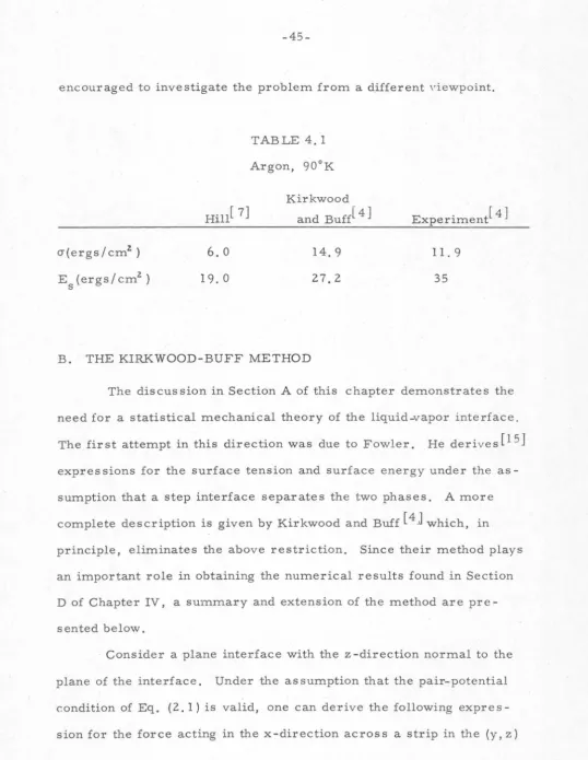
also calculated. Table (4. 1) compares Hill's results for argon at

90°K with those obtained from another method developed by Kirkwood

and Buff[ 4]. The latter method will be discussed in detail in the next

section.

It is clear that Hill's approach involves assumptions that are

difficult to justify. In fact, the assumptions present in Eqs. (4. 2)

and (4. 3) are simply not valid. We also note from Table (4. 1) that

there is considerable disagreement between the experimental results

[image:48.557.23.543.25.755.2]

encouraged to investigate the problem from a different \'iewpoint.

rJ(ergs/cm2 ) E (ergs/ cmz)

s

6.0

19.0

TABLE 4. I Argon, 90°K

Kirkwood and Buff[ 4 ]

14.9

27.2

B. THE KIRKWOOD-BUFF METHOD

Experiment[ 4 ]

11. 9

35

The discussion in Section A of this chapter demonstrates the need for a statistical mechanical theory of the liquid-vapor interface. The first attempt in this direction was due to Fowler. He derives

(1

5

J

expressions for the surface tension and surface energy under the as -sumption that a step interface separates the two phases. A more complete description is given by Kirkwood and Buff [ 4

.J

which, in principle, eliminates the above restriction. Since their method plays an important role in obtaining the numerical results found in Section D of Chapter IV, a summary and extension of the method are pre-sented below. [image:49.558.8.546.35.730.2]

plane of unit width in the y direction and extending from

in the z direction:

P.

L"

J.

+-P. P.

- L"

to

L"

2:

= -

k T

S

n ( 1 ) ( z }dz

+

x 1 1

P.

2

z

I.

S

dz

[

S

x lZ cp ' ( r )n ( z) ( z , r )dr ]

2 1 r 1Z 1 ""lZ ""lZ

p_ lZ

- Z"

-z-(4. 6)

where n( l)(z) is the density or first order distribution function as 1

in Chapter II, n(z )(z, r ) is the second order distribution function,

1 lZ .

r is the vector between points r and r , r is the distance

be-"'lZ "'1 ,...Z lZ

dcp(r )

tween r and r · and cp'(r )

=

lZ

"'l "'Z 1 Z dr is the derivative of the inter

-lZ

molecular potential. Obviously,

1

where

p'(z)

=

kTn(1 )(z)

-. 1 l

=

-s

2:

x

I_

_g

S

x 2

2 r

12

Z"

p'(z )dz

1 1

(z '

cp'(r )n 1(z,r )dr

12 l ,..,12 "'12 (4. 7)

From the mechanical definition of the surface tension, we must have

00

a =

S

(p-p'(z) )dz

1 1

-oo

(4. 8)

where p is the thermodynamic pressure of the system. If the

pair-potential condition holds, the pressure of the system may be written

p = kTnn -

J-Sr <P'(r

)n~

2 )(r }dr

.l'.. o 12 12 .l'.. 12 "'12 (4. 9)

or

p

=

kTn -

~

Sr <P

'(r )n (z. ) (r )dr

v 0 12 12. v 12 "i.2 (4.10)

where the subscripts l and v refer to the uniform liquid and uniform

':

.:

vapor states respectively. It is convenient to define the functions

n

1v and ni:) as

n_r.v 4 (z) = (l -H(z -z ) )n + H(z -z )n_{o v . o 1}

(4.II)

=

(1-H(z-z ))n(2)(r )+H(z-z )n

1(

2

)(r)

0 v 12. 0 12

where

l z

>

0

H(z) =

0 z

<

0

The surface z

=

z is an arbitrary Gibbs dividing surface.

There-o

fore, p can be written as

p

=

kTn

1v(z1

) -

~

Sr <P'(r

)n

1(z.) (r , z )dr

0 12 12 .. v 4 2 1 "12 (4. 12)

Substitution of Eqs. (4. 12) and (4. 7) into Eq. (4. 8) yields

er

=

-r(1 )kT

+

.!_

S

x122 <p1_{(r )r(}2 _{)(r )dr}

s 2 r 12. s "'12 ""'12

.

.

(4. 13)

12.

):c

nv 1s the uniform vapor density and n

where

and

r(l)

=

S

00

n (z )dz

s s 1 1

-co

00

,....

r( 2 ) ( r )

= \

n ( 2 ) ( z , r )dz

S lZ

J

S l ~z 1

-00

n (z )

=

n (l ) (z ) - IlA (z )

s 1 1 x.v 1

r(l ) is the Gibbs superficial density relative to the surface

s

One can see from Eq. (4. 13) that

a

is independent of z .

0

(4.14)

(4.15)

z

=

z .

0

If the pair-potential condition is satisfied, the functions

n(h)(r . . Ith) must satisfy the B.B.G.K. Y. equations. In particular

"'l

dz

1

or, because

=

+

1

s

zr1z cp'{r )n(z )(r 'z )dr

kT lZ ""lZ 1 ~12

lZ

S

z f{r )dr = 0

lZ lZ "'lZ

for arbitrary f{r ), lZ

dn (z)

s 1

dz

1

=

{n -nl )o (z -z )

+

kl

s

zr1z <P '{r )n (z )(z , r )dr

v · 1 o T

12 iz s 1 'lz -iz

(4.16)

Multiplication of Eq. (4. 17) by (z -z ) and integration from z = -co

1 0 1

to z =

+

oo gives

00

s

dn (z)

s

z

s

00

( z - z ) s 1 dz 1

_g_

cp 1 _{( r ) ( z - z )n ( z ) ( z , r )dz dr}

1 o dz 1 = k T r iz 1 o s i J'.z i "'1z

-oo 1 12 -00

or

00 .

\ ld d d

f

(

z -z )n ( z )) - n ( z )] dz

J

L

crz--i

i o s i s 1 1

-00 1

00

- 1_

s

zlZ

s

(Z )

=

kT r <P '(r ) (z -z )n (z , r )dz dr

lZ 1 0 S 1 ""'lZ 1 "'l Z

lZ _-oo

and by assuming lim z n (z ) - 0, we have that

z -+oo 1 s 1

where

l

or z --oo 1

r(l)

=

I

s

zrlZ cp'(r ){r(z)(r )} dr

s - kT lZ S "-'lZ

1 "'1z

lZ

00

{ r(Z ) }

=

s (

z - z )n ( z ) ( z ' r )dz

S 1 1 0 S 1 ""lZ 1

-00

Substituting Eq. (4.18) into Eq. (4.13), we obtain

(J=S-

1

- cp'(r >[z {r(z)(r

n

+~

r(z)(r >]dr

r iz iz s _{""'1z 1} c. s ""'1z ~12

lZ

The Gibbs surface energy is, by definition,

E = 2 1

S

cp(r )r(z )(r )dr

S 12. S "'1z ""lZ

(4. 18)

(4.19)

(4.20)

(4.21)

where in the definition of r( 2 )' is determined by the condition

z

0 00

C

(n(1)(z )-n )dz

+

J

1 v 1

S

(n(

1

)(z

1

)-n

1)dz1

= 0

-oo

In other words,

Thus,

a

z

0

and

z

0

is chosen so that r(l)

=

o.

s

E can be determined if n (1 )(z ) and

s l

are known. Unfortunately, these functions can be determined only by

solving the B.B.G.K. Y. equations. Progress can be made, however,

if one as sum es a particular n ( 1 )(z ) and n (2 )(z, r ) and then sub

-l 1 ""12

stitutes these quantities into Eqs. (4. 20) and (4. 21 ). The step

inter-face model is defined aB

n(2)(z,r)

g(2)(z,r) ₌ 1 ~12.

n(l )(z )n(1 )(z) =

1 ~12

1

z.

n v

gl (r 1)

g (r

v 12. )

z

>

0

l

z

<

0

1

z

>

1

z

<

1

glv(r 1) z ₁

<

g.lv(r 12. ) z ₁

>

0

0

0 '

0 '

where z

= 0 is the position of the step interface.

1

(4. 22)

z

>

0

2

z

<

0

2

(4.23)

z

>

0

z.

z

<

0

2

~:'

If we choose

':'If n(1 )(z) and n(z.

~z,

r ) are related by Eq. (4.16),then

a,

as

1 1 ~12

expressed by (4. 20),is independent of z

0 . For the step model,

a

is likewise independent of z . For a general model, however,

a

0

will depend on z . This problem is not present in the expression for

0

and r( z )(r ) can be calculated from relations s "'12

(4. 22) and (4. 23 ). Substituting the results into Eq. (4. 20), we obtain

cr

~ ~

s"'

r'<P'(r) {(n₁)'g

1(r)

+

(n)'g)r) - 2n1nvgl)r)}dr , ( 4. 24) 0

Since z = 0 is the surface where r( 1) = 0, expression (4. 21) for

0 s

the surface energy, with the step interface assumption, becomes

00

Es = -

~

S

r3 cp(r ){ (n_{1 )}2 g₁(r)

+

(nv)2g)r) - 2n₁nvg.t)r )}dr

0

(4. 25)

Kirkwood and Buff[ 4] assume and,in the low vapor density

limit,obtain

00

(J =

~

(n.l)2

S

r4cp'(r)g.l(r)dr

0

00

,.

Es= - ; (n₁)2

J

r3cp(r)g₁(r)dr

0

(4. 26)

(4. 27)

Equations (4. 26) and (4. 27) can be evaluated if the intermolecular

potential and the liquid pair-correlation function are known. Table

(4. l) contains the results calculated from Eqs. (4. 26) and (4. 27) for

Argon[ 4 ] at 90°K. Shoemaker, Paul, and Marc de Chazal[5] have

recently evaluated Eqs. (4. 26) and (4. 27) using more accurate g 1(r)

data for several simple liquid-vapor systems. Their results

com-pare favorably with experiment and will be presented in Section D

of this chapter.

[image:55.563.6.544.35.741.2]

surface tension, Eqs. (4. 20) and (4. 13) ,exists. Instead of substituting

Eqs. (4. 22) and (4. 23) into Eq. (4. 2 0) and evaluating the surface

tension, we could just as easily substitute these relations into Eq.

(4. 13). One then obtains, for the low-vapor-density approximation,

00

1T

z

r

-4,

a

= -

8

(n

1)

J

r <p'(r)g1(r)dr (4.28)

0

or exactly the negative of Eq. (4. 26). Since the surface tension

deriv-ed from Eq. (4. 26) is usually close to the experimental results, one

must conclude that the surface tension values derived from Eq. (4. 28)

are nonphysical . Fowler (l S]computes the surface tension for the

step interface model (low vapor density) by defining the surface

ten-sion to be one half the work of adheten-sion between two columns of liquid

phase of unit cross sectional area. His results are identical to those

derived from Eq. (4. 20) when the same approximations are employed.

Since the two definitions of the surface tension must be compatible,

one must consider

a

as defined by Eq. (4. 20) to be the proper expres

-sion to use with model assumptions like Eqs. (4. 22) and (4. 23). As a

final remark, we should note that Eq. (4. 21) for the surface energy is

free from any such ambiguity.

C. STRUCTURE OF THE INTERFACE

The structure of the liquid-vapor interface can be determined

if the distribution functions of classical statistical mechanics are

known. The most commonly suggested method of solution involves

Eq. (3. 20). The solution of the resulting system of two equations is

extremely difficult and must be accomplished numerically. To our

knowledge, no solution has been obtained for a nonuniform problem

such as the liquid-vapor interface.

There exists another set of equations, mentioned in Chapter

III,