ISSN Online: 2327-4085 ISSN Print: 2327-4077
DOI: 10.4236/jmmce.2018.63021 May 4, 2018 294 J. Minerals and Materials Characterization and Engineering
Modeling and Optimization of Galena
Dissolution in Hydrochloric Acid:
Comparison of Central Composite Design
and Artificial Neural Network
Ikechukwu A. Nnanwube
*, Okechukwu D. Onukwuli, Sunday U. Ajana
Department of Chemical Engineering, Nnamdi Azikiwe University, Awka, Nigeria
Abstract
Response surface methodology (RSM) and Artificial neural network (ANN) were used for the simulation and optimization of galena dissolution in hy-drochloric acid. The galena ore was characterized for structure elucidation using FTIR, SEM and X-ray diffraction spectroscopic techniques and the re-sults indicate that the galena ore exists mainly as lead sulphide (PbS). A feed-forward neural network model with Leverberg-Marquardt back propa-gating training algorithm was used to predict the response (lead yield). The leaching temperature, acid concentration, solid/liquid ratio, stirring rate and leaching time were defined as input variables, while the percentage yield of lead was labelled as output variable. The multilayer perceptron with architec-ture of 5-9-1 provided the best performance. All the process variables were found to have significant impact on the response with p-values of <0.0001. The performance of the RSM and ANN model showed adequate prediction of the response, with AAD of 0.750% and 0.295%, and R2 of 0.991 and 1.00, respec-tively. A non-dominated optimal response of 85.25% yield of lead at 343.96 K leaching temperature, 3.11 M hydrochloric acid concentration, 0.021 g/ml solid/liquid ratio, 362.27 rpm stirring speed and 87.37 min leaching time was es-tablished as a viable route for reduced material and operating cost using RSM.
Keywords
Galena Dissolution, Optimization, ANN Modelling, Hydrochloric Acid, RSM
1. Introduction
Lead is a naturally occurring metallic element usually associated with other ore
How to cite this paper: Nnanwube, I.A., Onukwuli, O.D. and Ajana, S.U. (2018) Modeling and Optimization of Galena Dissolution in Hydrochloric Acid: Com-parison of Central Composite Design and Artificial Neural Network. Journal of Min-erals and Materials Characterization and Engineering, 6, 294-315.
https://doi.org/10.4236/jmmce.2018.63021 Received: March 5, 2018
Accepted: May 1, 2018 Published: May 4, 2018
Copyright © 2018 by authors and Scientific Research Publishing Inc. This work is licensed under the Creative Commons Attribution International License (CC BY 4.0).
http://creativecommons.org/licenses/by/4.0/
DOI: 10.4236/jmmce.2018.63021 295 J. Minerals and Materials Characterization and Engineering minerals such as pyrite, sphalerite, quartz and barite. Trace amounts of other elements including gold are sometimes found with lead ore. The most common ore mineral of lead is galena (PbS) also known as lead sulphide. Lead’s high den-sity, atomic number, and formability form the basis for use of lead as a barrier that absorbs sound, vibration, and radiation. Lead has no natural resonance fre-quencies; as a result, sheet-lead is used as a sound deadening layer in the walls, floors, and ceilings of sound studies. Organ pipes are often made from a lead alloy, mixed with various amounts of tin to control the tone of each pipe. Lead is an established shielding material from radiation in nuclear science and in X-ray rooms due to its denseness and high attenuation coefficient. Molten lead has been used as a coolant for lead-cooled fast reactors [1]. The single most important commercial use of lead is in the manufacture of lead-acid storage batteries.
Response surface methodology (RSM) was developed by Box and Wilson [2]
to enable the improvement of manufacturing processes in the chemical industry. It focused on optimizing chemical reactions in order to obtain, e.g., high yield and purity at low costs. This was accomplished through the use of sequential experimentation, involving factors such as temperature, pressure, duration of reaction, and proportion of reactants. The same methodology can be applied to model or optimize any response that is affected by the levels of one or more quantitative factors.
The most popular RSM is the central composite design (CCD). A CCD has three groups of design points: 1) two-level factorial or fractional factorial design points, 2) axial points (sometimes called star points), and 3) centre points. CCDs are designed to estimate the coefficient of a quadratic model. All point descrip-tion is in terms of coded values of the factors.
Artificial Neural Network (ANN) is an empirical tool, which is analogous to the behavior of biological neural structures [3]. Neural networks are powerful tools that have the abilities to identify underlying highly complex relationships from input-output data only [4]. For the past two decades, artificial neural net-works (ANNs), and, in particular, feed-forward artificial neural netnet-works (FANNs), have been extensively studied to present process models, and their use in industry has been rapidly growing [5].
DOI: 10.4236/jmmce.2018.63021 296 J. Minerals and Materials Characterization and Engineering
2. Materials and Methods
2.1. Material
Sample Mining and Preparation
The galena ore used for this study was collected from Abakaliki, Enyigba mining site in Ebonyi State of Nigeria. The galena ore was finely pulverized and sieved with a 75 µm size sieve. All experiments were performed with the 75 µm frac-tion. HCl solutions were prepared from analytical grade reagents with deionized water.
2.2. Methods
2.2.1. Spectrophotometric Analysis
The X-ray fluorometer (XRF), X-supreme 600 oxford instruments was used for the elemental analysis of the ore. The mineralogical analysis of the ore was done using ARL X’TRA X-ray Diffractometer, Thermoscientific with the serial num-ber 197492086 with CuKα (1.54 Å) radiation generated and 40 mA and 45 kV. This unit comprises of a single compact cabinet. The cabinet houses a high speed, high precision Goniometer; high efficiency generator (X-ray) and an au-tomatic sample loading facility.
The petrographic slides of galena ore were prepared using Epoxy and Lakeside 70 media according to the method of Hutchison [6].
2.2.2. FTIR and SEM Analysis
FTIR analysis was carried out using Buck Scientific M530 Infrared Spectropho-tometer. SEM analysis was carried out using Q250 by FEI model from the Neth-erlands.
2.2.3. Experimental Procedure
Leaching experiments were performed in a 500 ml glass reactor fitted with a condenser to prevent losses through evaporation. The two major variables (heat and stirring rate) necessary for accelerating the rate of chemical reaction was provided by the aid of a magnetically-stirred hot plate (Model 78HW-1). For every leaching experiment, the solution mixture was freshly prepared by dis-solving the required mass of the ore sample in the acid solution at the required temperature. At the end of each reaction time, the undissolved materials in the suspension was allowed to settle and separated by filtration. The resulting solu-tions were diluted and analyzed for lead using atomic absorption spectrophoto-meter (AAS).
The mole fraction of lead passing into the solution from galena was calculated by the formula given in Equation (1), where x designates quantity dissolution.
Amount of Pb passing into the solution Amount of Pb in original sample
x= (1)
2.2.4. Design of Experiment
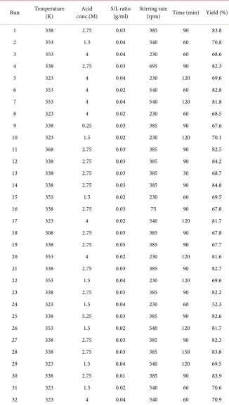
DOI: 10.4236/jmmce.2018.63021 297 J. Minerals and Materials Characterization and Engineering were investigated using RSM combined with five-level, five factor fractional fac-torial design as established by Design Expert software (10.0 rented version). The process variables were leaching temperature, acid concentration, solid/liquid ra-tio, stirring rate and leaching time. The response variable was chosen as% yield of lead. The factor levels were coded as −α, −1, 0, +1 and +α. The range and le-vels are shown in Table 1.
A total of 32 runs were carried out to optimize the process variables and expe-riments were performed according to the actual experimental design matrix shown in Table 2. The experiments were performed randomly to avoid systemic error. The results were analyzed using the analysis of variance (ANOVA), con-tour, and response surface plots. In RSM, the most widely used second-order polynomial equation (Equation (2)) developed to fit the experimental data and identify the relevant model terms may be written as:
2 0
1 1
k k
i i ij i j ii i
i i j i
Y β β x β x x β x ε
= < =
= +
∑
+∑∑
+∑
+ (2)where Y is the predicted response variable which is the% yield of lead in this study, β0 is the constant coefficient, βi is the i
th linear coefficient of the input
variable xi, βii is the i
th quadratic coefficient of the input variable
i
x , βij is
the different interaction coefficients between the input variables xi and xj
and ε is the error of the model.
3. Results and Discussion
3.1. Results of Characterization Studies
3.1.1. Elemental Composition by XRFThe results of the elemental composition of galena by X-ray fluorescence tech-nique showed that the galena mineral exist mainly as PbS with metals such as Na, Mg, Al, Ca, Fe and Zn occurring as minor elements, and K, Cr, and Sr as traces. The elemental analysis gave Pb (60.01%), S (14.66%), Fe (4.32%), Na (3.78%), Si (7.69%), Mg (1.21%), Al (1.94%), P (1.37%), Cl (1.19%), K (0.09%), Ca (1.99%), Cr (0.01%), Mn (0.49%), Zn (1.22%), and Sr (0.04%).
3.1.2. Phase Studies by XRD
[image:4.595.209.540.601.724.2]The analysis of galena by X-ray diffraction gives a better description in terms of
Table 1. Levels of independent variables for CCD experimental design.
Independent variable Unit Symbol Coded variable levels
−α −1 0 +1 +α Leaching temperature K X1 308 323 338 353 368
Acid concentration M X2 0.25 1.5 2.75 4.0 5.25
Solid/liquid ratio min X3 0.01 0.02 0.03 0.04 0.05
Stirring rate g/ml X4 75 230 385 540 695
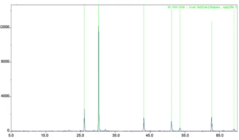
DOI: 10.4236/jmmce.2018.63021 298 J. Minerals and Materials Characterization and Engineering the mineral phases present in the ore. Table 2 present the results of the X-ray diffractogram of the ore and shows that the ore exist mainly as lead sulphide (PbS).
[image:5.595.207.540.202.339.2]The galena ore gave three major peaks at 2.96, 3.42, and 2.09 Å, respectively as shown in Figure 1. All these supported the results of the elemental analysis by XRF.
Table 2. The X-ray diffraction data of the galena ore showing the angle 2θ and d-values of the compounds identified, with their relative intensity (%).
2θ d-Value (Å) Compound Intensity (%) JCPDS file No. 26.03 3.42 Galena (PbS) 93.99 01-078-1056 30.15 2.96 Galena (PbS) 100.00 01-078-1056 43.16 2.09 Galena (PbS) 65.77 01-078-1056 51.10 1.79 Galena (PbS) 38.14 01-078-1056 53.55 1.71 Galena (PbS) 20.72 01-078-1056 62.68 1.48 Galena (PbS) 8.71 01-078-1056 69.06 1.36 Galena (PbS) 12.91 01-078-1056
JCPDS File No.: Joint Committee on Power Diffraction Standards File Number.
Figure 1. X-ray diffraction pattern of galena ore.
3.1.3. FTIR Analysis of Galena
[image:5.595.60.543.359.642.2]DOI: 10.4236/jmmce.2018.63021 299 J. Minerals and Materials Characterization and Engineering Figure 2. FTIR spectrum of galena ore.
attributed to O-H bending. The bands at 3519 cm−1, 3353 cm−1 and 2564 cm−1 are attributed to N-H stretching. The band at 2564 cm−1 which is attributed to S-H stretching confirms the presence of sulphur in the ore. The band at 1634 cm−1 is attributed to Si-O and Al-O stretching while the band at 1634 cm−1 is also attributed to Al-O-H stretching.
The FTIR result is in agreement with XRF and XRD results which confirmed the presence of the minerals detected.
3.1.4. SEM Analysis of Galena
The scanning electron micrograph (SEM) of galena ore was obtained with mag-nifications of 240×, 520×, 1000×, and 1500× respectively as shown in Figure 3. The average cell diameter of the ore ranges from 8 to 62 µm while the average cell density ranges from 0.0042 to 1.13 cells/mm. The results indicate that the ore particles are very cohesive, forming an aggregate mass that appeared to have been formed by several flaky particles stacked together in form of agglomerates
DOI: 10.4236/jmmce.2018.63021 300 J. Minerals and Materials Characterization and Engineering
(a) (b)
[image:7.595.58.538.68.591.2](c) (d)
Figure 3. SEM images of galena ore showing magnifications of 240× (a), 520× (b), 1000× (c), and 1500× (d) respectively.
The central composite design (CCD) for the leaching of lead from galena us-ing hydrochloric acid is shown in Table 3 with the experimental values.
3.2. RSM Modelling
DOI: 10.4236/jmmce.2018.63021 301 J. Minerals and Materials Characterization and Engineering Table 3. Fractional central composite design for galena dissolution in hydrochloric acid (HCl).
Run Temperature (K) conc.(M) Acid S/L ratio (g/ml) Stirring rate (rpm) Time (min) Yield (%) 1 338 2.75 0.03 385 90 83.8 2 353 1.5 0.04 540 60 70.8 3 353 4 0.04 230 60 68.6 4 338 2.75 0.03 695 90 82.3 5 323 4 0.04 230 120 69.6 6 353 4 0.02 540 60 82.8 7 353 4 0.04 540 120 81.8 8 323 4 0.02 230 60 68.5 9 338 0.25 0.03 385 90 67.6 10 323 1.5 0.02 230 120 70.1 11 368 2.75 0.03 385 90 82.5 12 338 2.75 0.03 385 90 84.2 13 338 2.75 0.03 385 30 68.7 14 338 2.75 0.03 385 90 84.8 15 353 1.5 0.02 230 60 69.5 16 338 2.75 0.03 75 90 67.8 17 323 4 0.02 540 120 81.7 18 308 2.75 0.03 385 90 67.8 19 338 2.75 0.05 385 90 67.7 20 353 4 0.02 230 120 81.6 21 338 2.75 0.03 385 90 82.7 22 353 1.5 0.04 230 120 69.6 23 338 2.75 0.03 385 90 82.2 24 323 1.5 0.04 230 60 52.3 25 338 5.25 0.03 385 90 82.6 26 353 1.5 0.02 540 120 81.7 27 338 2.75 0.03 385 90 82.3 28 338 2.75 0.03 385 150 83.8 29 323 1.5 0.04 540 120 69.5 30 338 2.75 0.01 385 90 83.9 31 323 1.5 0.02 540 60 70.6 32 323 4 0.04 540 60 70.9
experi-DOI: 10.4236/jmmce.2018.63021 302 J. Minerals and Materials Characterization and Engineering mental runs were quite unique, indicating that each of the factors have consid-erable effect on the response.
3.3. Statistical Analysis
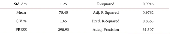
[image:9.595.206.541.493.578.2]To determine the adequacy of the models depicting the removal of lead by the dissolution of galena in hydrochloric acid, two different tests, i.e. the lack of fit test and the model summary statistics, were conducted. From the lack of fit test, the highest order polynomial with non-significant p-value and is not aliased would normally be chosen. This test is used in the numerator in an F-test of the null hypothesis and indicates whether a proposed model fits well or not. It com-pares the variation around the model with pure variation within replicated ob-servations and measures the adequacy of the model based on response surface analysis [8]. The results from the lack of fit test indicated that the 2FI, linear and the cubic model (aliased) did not provide a good description of the experimental data. The results are tabulated in Table 4. From the model summary statistics, it can be seen that the R-squared, adjusted R-squared and the predicted R-squared values for the quadratic model (0.9916, 0.9762, and 0.8565) showed a better cor-relation when compared with the cubic model (0.9948, 0.9732 and −1.4789) and the linear model (0.7281, 0.6758 and 0.6545) as shown in Table 5. The measure of how efficient the variability in the actual response values can be explained by the experimental variables and their interactions is given by the R-squared value. If the R-squared predicted and adjusted are too far from each other, there may be a problem with either the data or the model [8]. The results are tabulated in
Table 5. The afore-mentioned results indicate that the quadratic model provided an excellent explanation for the relationship between the independent variables and the corresponding response. With respect to these results, the effect of each
Table 4. Lack of fit tests.
Source Sum of squares df Mean Square F Value p-value Remarks Linear 545.26 21 25.96 22.10 0.0014 Inadequate
2FI 523.36 11 47.58 40.50 0.0004 Inadequate Quadratic 11.22 6 1.87 1.59 0.3132 Adequate
Cubic 4.62 1 4.62 3.93 0.1041 Aliased
[image:9.595.207.540.624.710.2]df = degree of freedom.
Table 5. Model summary statistics.
Source Std. Dev. R-Squared Adjusted R-Squared Predicted R-Squared PRESS Linear 4.60 0.7281 0.6758 0.6545 700.34 2FI 5.75 0.7389 0.4942 −3.0651 8240.35 Quadratic 1.25 0.9916 0.9762 0.8565 290.93
Cubic 1.32 0.9948 0.9732 −1.4789 5024.90
DOI: 10.4236/jmmce.2018.63021 303 J. Minerals and Materials Characterization and Engineering parameter was evaluated using the quadratic model as shown in Table 6.
The second-order model tested at the 95% confidence level obtained for ex-traction of lead from galena is shown in Equation (3):
1 2 3 4 5 1 2
1 3 1 4 1 5 2 3 2 4
2 5 3 4 3 5 4 5
2 1
2 2 2 2
2 3 4 5
Yield 83.52 3.44 3.39 3.57 3.71 3.41 0.31
0.24 0.28 0.35 0.37 0.14
0.24 0.36 0.26 0.77 2.23
2.25 2.07 2.26 1.96
X X X X X X X
X X X X X X X X X X
X X X X X X X
X X X X X X = + + − + + − + − − + − − + − − − − − − − (3)
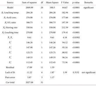
[image:10.595.208.538.428.721.2]The results were analyzed by using the analysis of variance (ANOVA) suitable for experimental design used and shown in Table 6. The ANOVA of the quad-ratic regression model indicates that the model is significant. The model F-value of 64.67 implied the model to be significant and there is only 0.01% chance that an F-value this large could occur due to noise. The F-value of the independent variables X1, X2, X3, X4, and X5 were estimated as 182.94, 177.66, 197.39, 212.39 and 179.41 respectively, showing that the effects of most independent variables on the dependent variable were significantly high. Model F-value was calculated as ratio of Adj. mean square of the regression and Adj. mean square of the re-sidual. The model P-value (Prob. > F) is very low which shows that the model is significant. The P-values were used as a tool to check the significance of each of the model coefficients. The smaller the P-value the more significant is the cor-responding coefficient. Values of P < 0.05 indicate the model terms to be sig-nificant. The values of P for the coefficients estimated indicate that among the
Table 6. ANOVA for Response surface reduced quadratic model.
Source Sum of squares df Mean Square F Value p-value Remarks Model 2009.99 20 100.5 64.67 <0.0001 significant X1-Leaching temp. 284.28 1 284.28 182.94 <0.0001
X2-Acid conc. 276.08 1 276.08 177.66 <0.0001
X3-S/L ratio 306.73 1 306.73 197.39 <0.0001
X4-Stirring rate 330.04 1 330.04 212.39 <0.0001
X5-Leaching time 278.80 1 278.80 179.41 <0.0001
4 5
X X 9.61 1 9.61 6.18 <0.0302
2 1
X 146.26 1 146.26 94.12 <0.0001
2 2
X 147.90 1 147.26 95.18 <0.0001
2 3
X 125.75 1 125.75 80.92 <0.0001
2 4
X 149.55 1 149.55 96.24 <0.0001
2 5
X 112.45 1 112.45 72.36 <0.0001
Residual 17.09 11 1.55
Lack of fit 11.22 6 1.87 1.59 0.3132 not significant Pure error 5.87 5 1.17
DOI: 10.4236/jmmce.2018.63021 304 J. Minerals and Materials Characterization and Engineering tested variables used in the design, X1, X2, X3, X4, X5, X4X5, X12,
2 2
X , X32, 2 4
X ,
2 5
X (where X1 = leaching temperature, X2 = acid concentration, X3 = solid/liquid ratio, X4 = stirring rate, and X5 = leaching time) are significant model terms. The “Lack of Fit F-value” of 1.59 implies that the Lack of Fit is not significant relative to the pure error. There is a 31.32% chance that a “Lack of Fit F-value” this large could occur due to noise. Non-significant lack of fit is good because it indicates that the model is well fitted. Since many insignificant model terms have been eliminated, the improved model can be used to predict effec-tively, the responses of the percentage recovery of lead from galena. The model equation with the significant coefficient is shown in Equation (4).
1 2 3 4 5 4 5
2 2 2 2 2
1 2 3 4 5
Yield 83.52 3.44 3.39 3.57 3.71 3.41 0.77 2.23 2.25 2.07 2.26 1.96
X X X X X X X
X X X X X
= + + − + + −
− − − − − (4)
In terms of the actual factors the model equation (Equation (5)) is as follows:
2
Yield 1244.09 7.05 Leaching temperature 16.19 Acid concentration 98.32 Solid / Liquid ratio 0.15 Stirring rate
0.82 Leaching time 1.67E 004 Stirring rate Leaching time 9.92E 003 Leaching temperature 1
= − + ∗ + ∗
+ ∗ + ∗
+ ∗ − − ∗ ∗
− − ∗ − 2
2 2
2
.44 Acid concentration – 20704.55 Solid / Liquid ratio 9.40E 005 Stirring rate – 2.18E 003 Leaching time
∗
∗ − − ∗
− ∗
(5)
The CV called coefficient of variation which is defined as the ratio of the standard deviation of estimate to the mean value of the observed response is in-dependent of the unit. It is also a measure of reproducibility and repeatability of the models [9] [10]. The results indicated the CV value of 1.65% which illus-trated that the model can be considered reasonably reproducible [9]. The signal to noise ratio which is given as the value of the adequate precision is 31.307 as shown in Table 7. This indicates that an adequate relationship of signal to noise ratio exists. The result shows that the model can be used to navigate the design space.
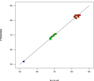
[image:11.595.207.540.651.719.2]The data were also analyzed to check the correlation between the experimental and predicted dissolution yield (Y%), as shown in Figure 4. The experimental values were the measured response data for the runs designed by the CCD model, while the predicted values were obtained by calculation from the quad-ratic equation. It can be seen from Figure 4 that the data points on the plot were reasonably distributed near to the straight line (R2 = 0.9916), indicating a good relationship between the experimental and predicted values of the response. This
Table 7. Summary of regression values.
DOI: 10.4236/jmmce.2018.63021 305 J. Minerals and Materials Characterization and Engineering Figure 4. Plot of predicted values versus experimental values.
shows that the model chosen is appropriate and that the central composite de-sign (CCD) can be used to perform the optimization operation of the process.
3.4. Combined Effects of Operating Parameters on the Response
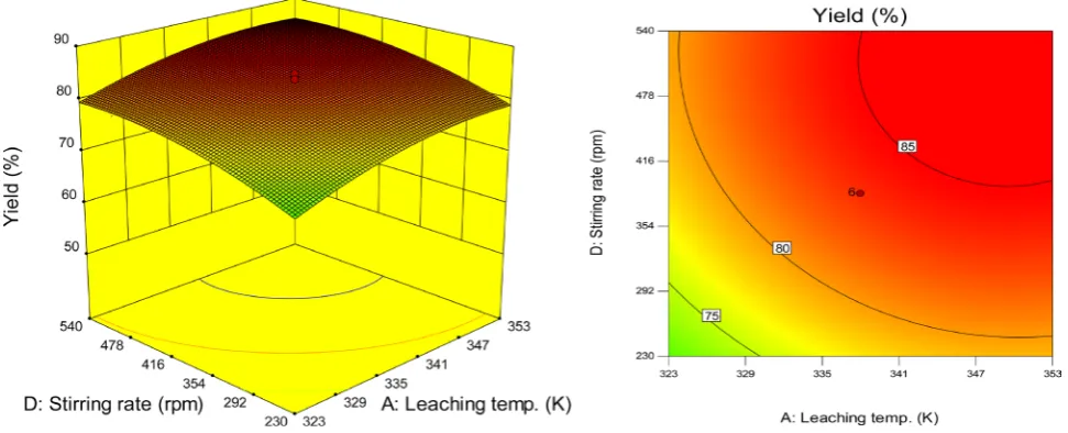
The dissolution process for the extraction of lead from galena was analyzed based on the various solutions obtained at possible reaction conditions from the model predictive Equation (2). RSM was considered appropriate owing to its flexibility in navigating the design space. The model equations were solved for the various interaction effects on lead yield considering at any instance the in-teraction between two factors only, assuming the other variables are set at their mean coded value of zero (0). The combined effects of adjusting the process variables within the design space were monitored using the 3D surface plots and contour plots.As the leaching temperature is increased from 326 K to 342 K, the percentage recovery of lead increased from 75% to 85% as seen in Figure 5. This linear rela-tionship is as a result of increase in kinetic energy with higher temperature which allows the solvent molecules to more effectively break apart the solute molecules that are held together by intermolecular attractions, hence increasing the diffusion rate from the solid bulk phase into the solvent region. The same trend was observed in Figures 6-8. The results obtained here are in agreement with the results of statistical analyses shown in Table 6 which reveals that the quadratic effect of temperature (X1 squared) on the response is significant within the factor range of the experiment with a p-value of <0.0001. This is in line with
Actual
P
red
ic
ted
50 60 70 80 90
DOI: 10.4236/jmmce.2018.63021 306 J. Minerals and Materials Characterization and Engineering Figure 5. 3D and contour plots on the effect of leaching temperature and acid concentration on % yield.
Figure 6. 3D and contour plot of the effect of leaching temperature and solid/liquid ratio on % yield.
[image:13.595.57.543.513.710.2]DOI: 10.4236/jmmce.2018.63021 307 J. Minerals and Materials Characterization and Engineering Figure 8. 3D and contour plot of the effect of leaching time and leaching temperature on % yield.
the report of several researchers [11] [12] [13] who agree that increase in tem-perature substantially increases the dissolution rate of solutes.
As the acid concentration is increased from 1.8 M to 3.18 M, the percentage recovery of lead increased from 75% to 85% as seen in Figure 5. This is attrib-uted to the increase in the diffusion rates of Pb2+ from the solid to the solution as the concentration and diffusion of hydronium ion rises. The same trend was ob-served in Figures 9-11.
A plot for the combined interactive effects of reaction temperature and
solid/liquid ratio on the recovery of lead is shown in Figure 6. As the
solid/liquid ratio is decreased from 0.039 to 0.028 g/ml, the percentage recovery of lead increased from 75% to 85%. This could be attributed to the decrease in the fluid reactant per unit weight of the solid [11]. The same trend was observed in Figure 9, Figure 12 and Figure 13.
The plot for the combined effects of leaching temperature and stirring rate on the recovery of lead is shown in Figure 7. As the stirring rate is increased from 270.4 rpm to 429.5 rpm, the percentage recovery of lead increased from 75% to 85%. This could be attributed to the decrease in the thickness of the film layer as the stirring rate is increased [11]. The same trend was observed in Figure 10,
Figure 12 and Figure 14.
As the leaching time is increased from 65 min to 93.2 min, the percentage re-covery of lead increased from 74% to 84% as seen in Figure 8. The same trend was observed in Figure 11, Figure 13 and Figure 14. The results obtained above also indicate that the quadratic effects of acid concentration, solid/liquid ratio, stirring rate and leaching time on response are also very significant within the factor range of the experiment with p-values of <0.0001.
3.5. ANN Modeling
DOI: 10.4236/jmmce.2018.63021 308 J. Minerals and Materials Characterization and Engineering Figure 9. 3D and contour plot of the effect of solid/liquid ratio and acid concentration on % yield.
[image:15.595.50.544.71.268.2]Figure 10. 3D and contour plot of the effect of stirring rate and acid concentration on % yield.
[image:15.595.58.543.503.694.2]DOI: 10.4236/jmmce.2018.63021 309 J. Minerals and Materials Characterization and Engineering Figure 12. 3D and contour plot of the effect of stirring rate and solid/liquid ratio on % yield.
Figure 13. 3D and contour plot of the effect of leaching time and solid/liquid ratio on % yield.
[image:16.595.56.547.519.706.2]DOI: 10.4236/jmmce.2018.63021 310 J. Minerals and Materials Characterization and Engineering which attempt to simulate some of the neurological processing abilities of the human brain [14]. They can be considered as a nonlinear regression tool for making a relationship between input and output variables. Multilayer percep-tron, radial basis function networks, linear networks, Bayesian networks (gene-ralized regression), and Kohonen networks (probabilistic regression) are the most well-known ANN types.
Multilayer perceptrons (MLP) is perhaps the most popular network architec-ture in use today [15]. Neurons perform a weighed sum of their inputs and pass it through a transfer function f to produce their output. The MLP model used in this work was developed in MATLAB (The math works Inc. 2007b). For galena dissolution in HCl, the selected MLP model had three layers, where the first had five input units representing the process independent variables (tempera-ture, acid concentration, solid/liquid ratio, stirring rate and leaching time), the second layer had nine hidden units, and the third layer had one output unit representing the percentage yield of lead. The MLP architecture is shown in
Figure 15.
3.5.1. Network Training
[image:17.595.209.539.515.692.2]In order to reduce the deviations of predictions from experimental values, a trial and error technique was employed to determine the adequate number of neu-rons required in the hidden layer. 70% of experimental results was used to train the network, 20% was used to validate the training while the remaining 10% was used for testing. After the selection of the hidden number of neurons, a number of runs were performed to get the best possible weights in error back propaga-tion and the final selected network architecture was trained for 9 iterapropaga-tions. The mean square error of the trained network is 1.36847e−1 with a regression coeffi-cient of 0.998520. The performance plots of the trained network as well as the regression plots for the training and validation are shown in the Figure 16 and
Figure 17 respectively.
DOI: 10.4236/jmmce.2018.63021 311 J. Minerals and Materials Characterization and Engineering Figure 16. Performance plot for galena dissolution in HCl ANN model.
Figure 17. Regression plots for the training (a) and validation (b) for galena dissolution in HCl ANN model using 5 input va-riables, 9 processing elements in the hidden layer and 1 output variable.
3.5.2. Comparison of RSM and ANN
A comparison between Artificial Neural Network (ANN) and Response Surface Methodology was carried out using the Absolute average deviation (AAD) and Coefficient of determination observed for both models. The AAD observed for both models gives an indication of how accurate the model predictions can be
[image:18.595.87.513.369.593.2]DOI: 10.4236/jmmce.2018.63021 312 J. Minerals and Materials Characterization and Engineering
( )
artpred artexp1 artexp
1
AAD % 100
n
i
R R
n = R
−
= ×
∑
(6)where n is the number of sample points, Rartpred is the predicted value of lead
dissolution and Rartexp is the experimentally determined value for lead
dissolu-tion [16].
The linear fit model (Y =((1.0) * T + (0.22)) generated by the trained outputs vs target plots shown in Figure 17 was used to predict the ANN model values. Where Y = the ANN model value, T (Target) = the experimental value used to generate the corresponding ANN value. The graph of the correlation between the experimental values and the predictions by RSM and ANN is shown in Fig-ure 18.
From the AAD estimation, RSM gave an AAD of 0.750% and ANN model gave an AAD of 0.295%. From the graph in Figure 18, the coefficient of deter-mination for the RSM model is 0.991, while that of ANN is 1.0. These values are a measure of how close the predicted value of the response is to the actual expe-rimental values. The closer each of these values is to 1, the better the prediction. Since the value of COD for both RSM and ANN are approximately equal to 1, it is evident that both models could efficiently predict the recovery of lead from galena [13]. RSM was then adopted for the optimization studies.
3.6. Process Optimization Using CCD
[image:19.595.217.534.482.714.2]The optimization exercise for the dissolution process was conducted separately using the flexibility of the design expert tool function. Equation (4) was solved for the best solutions such that the responses (Yn) are maximized within the de-sign space. No unique solutions were possible. A usual approach, which involves selecting the best solution based on economic considerations, was adopted and
DOI: 10.4236/jmmce.2018.63021 313 J. Minerals and Materials Characterization and Engineering the chosen optimal solutions are presented in Table 8. The selection of desired optimum solution of Table 8 was mainly influenced by the cost of reagents and energy. By using the numerical optimization technique which is a feature of CCD in the design expert software, a combination of factors that concurrently satisfy the requirements placed on each of the responses and factors could be determined by the software [13]. In choosing the goal for each of the factors for the numerical optimisation, a number of considerations were made. The signifi-cance of each of the factors on the final response was the most important con-sideration. The response was set at maximum goal, all other factors were kept in range apart from the reaction time which was set to a minimum goal target. Based on these, the software predicted optimum reaction conditions with a de-sirability of 1.00 tabulated in Table 8.
In order to confirm the accuracy of this model, an experimental run was con-ducted under these optimal conditions. The experimentally obtained value for the% yield of lead was 84.54% and this was in reasonable agreement with that of CCD model of design expert (85.25%) as shown in Table 9. A non-dominated optimal response of 85.25% yield of lead at 343.96 K leaching temperature, 3.11 M hydrochloric acid concentration, 0.021 g/ml solid/liquid ratio, 362.27 rpm stirring speed and 87.37 min leaching time was established as a viable route for reduced material and operating cost using RSM.
4. Conclusion
The optimum conditions for the extraction of lead from galena were investigated in this work. Response surface methodology (RSM) and Artificial neural net-work (ANN) were used for the modeling and optimization of process parame-ters. The performances of the models were estimated on the basis of correlation coefficients, absolute average deviation (AAD) and mean square error (MSE). The experimental data for the central composite design (CCD) of RSM were fit-ted using the second-order polynomial equation. The best multilayer perceptron (MLP) model of ANN had nine neurons and a logistic sigmoid activation func-tion in the hidden layer. CCD and ANN regression coefficients were obtained to be 0.991 and 1.00 respectively showing good agreement with the experimental
Table 8. CCD optimum predicted condition.
Leaching
[image:20.595.207.540.664.729.2]temperature concentration Acid Solid/Liquid ratio Stirring rate Leaching time % Yield 343.96 K 3.11 M 0.021 g/ml 363.27 rpm 87.37 min 85.25%
Table 9. Results of validation experiments.
Leaching
DOI: 10.4236/jmmce.2018.63021 314 J. Minerals and Materials Characterization and Engineering data. The absolute average deviation (AAD) for RSM and ANN was obtained as 0.750% and 0.295% respectively. Both methodologies proved to be quick and useful tools for the optimization of lead recovery from galena. The higher value of the correlation coefficient and lower values of AAD and MSE for the MLP model indicate that the MLP of ANN provides better prediction of experimental data than the CCD model.
References
[1] Tucek, K., Carlsson, J. and Wider, H. (2006) Comparison of Sodium and Lead-Cooled Fast Reactors Regarding Reactor Physics Aspects, Severe Safety and Economical Issues. Nuclear Engineering and Design, 236, 1589-1598.
https://doi.org/10.1016/j.nucengdes.2006.04.019
[2] Box, G.E.P. and Wilson, K.B. (1951) On the Experimental Attainment of Optimum Conditions. Journal of the Royal Statistical Society: Series B, 13, 1-45.
[3] Yao, H.M., Vuthaluru, H.B., Tade, M.O. and Djukanovic, D. (2005) Artificial Neur-al Network-Based Prediction of Hydrogen Content of CoNeur-al in Power Station Boilers. Fuel, 84, 1535-1542.https://doi.org/10.1016/j.fuel.2005.02.019
[4] Haykin, S. (1999) Neural Networks, a Comprehensive Foundation. 2nd Edition, Prentice Hall, Upper Saddle River.
[5] Ungar, L.H., Hartiman, E.J., Keeler, J.D. and Martin, G.D. (1996) Process Modeling and Control using Neural Networks. American Institute of Chemical Engineers Symposium Series, 96, 57-66.
[6] Hutchison, C.S. (1974) Laboratory Handbook of Petrography Techniques. John Wiley and Sons Inc., New York, 1-14.
[7] Bendou, S. and Amrani, M. (2014) Effect of Hydrochloric Acid on the Structural of Sodic-Bentonite Clay. Journal of Minerals and Materials Characterization and En-gineering, 2, 404-413.https://doi.org/10.4236/jmmce.2014.25045
[8] Taran, M. and Aghaie, E. (2015) Designing and Optimization of Separation Process of Iron Impurities from Kaolin by Oxalic Acid in Bench-Scale Stirred-Tank Reactor. Applied Clay Science, 107, 109-116.https://doi.org/10.1016/j.clay.2015.01.010 [9] Chen, G., Chen, J., Srinivasakannan, C. and Peng, J. (2011) Application of Response
Surface Methodology for Optimization of the Synthesis of Synthetic Rutile from Ti-tania Slag. Applied Surface Science, 258, 3068-3073.
https://doi.org/10.1016/j.apsusc.2011.11.039
[10] Chen, G., Xiong, K., Peng, J. and Chen, J. (2010) Optimisation of Combined Me-chanical Activation Roasting Parameters of Titania Slag Using Response Surface Methodology. Advanced Powder Technology, 21, 331-335.
https://doi.org/10.1016/j.apt.2009.12.017
[11] Ajemba, R.O. and Onukwuli, O.D. (2012) Determination of the Optimum Dissolu-tion CondiDissolu-tions of Ukpor Clay in Hydrochloric Acid Using Response Surface Me-thodology. International Journal of Engineering Research & Applications, 2, 732-742.
[12] Baba, A.A. and Adekola, F.A. (2010) Hydrometallurgical Processing of a Nigerian Sphalerite in Hydrochloric Acid: Characterization and Dissolution Kinetics. Hy-drometallurgy, 101, 69-75.https://doi.org/10.1016/j.hydromet.2009.12.001
DOI: 10.4236/jmmce.2018.63021 315 J. Minerals and Materials Characterization and Engineering and ANN Comparative Analysis. South African Journal of Chemical Engineering, 24, 43-54.https://doi.org/10.1016/j.sajce.2017.06.003
[14] Achanta, A.S., Kowalski, J.G. and Rhodes, C.T. (1995) Artificial Neural Networks: Implications for Pharmaceutical Sciences. Drug Development and Industrial Phar-macy, 21, 119-155. https://doi.org/10.3109/03639049509048099
[15] Salmasi, M., Mahdavi-Nasab, H. and Pourghassem, H. (2011) Evaluating the Per-formance of MLP Neural Network and GRNN in Active Cancellation of Sound Noise. Canadian Journal on Artificial Intelligence, 2, 28-33.