The Dynamics and Distribution of Angular Momentum in
HiZELS Star – Forming Galaxies at
z
= 0.8 – 3.3
S. Gillman,
1?A. M. Swinbank,
1,2A. L. Tiley,
1C. M. Harrison,
9Ian Smail,
1,2U. Dudzeviˇ
ci¯
ut˙e,
1R. M. Sharples,
1,3P. N. Best,
7R. G. Bower
1,2R. Cochrane,
7,8D. Fisher,
6J. E. Geach,
12K. Glazebrook,
6Edo Ibar,
4J. Molina,
14D. Obreschkow,
10,11M. Schaller,
2D. Sobral,
5S. Sweet,
6J. W. Trayford
2,13T. Theuns
21Centre for Extragalactic Astronomy, Durham University, South Road, Durham, DH1 3LE UK 2Institute for Computational Cosmology, Durham University, South Road, Durham DH1 3LE UK 3Centre for Advanced Instrumentation, Durham University, South Road, Durham DH1 3LE UK
4Instituto de F´ısica y Astronom´ıa, Universidad de Valpara´ıso, Avda. Gran Breta˜na 1111, Valpara´ıso, Chile 5Department of Physics, Lancaster University, Lancaster, LA1 4BY, UK
6Centre for Astrophysics and Supercomputing, Swinburne University of Technology, PO Box 218, Hawthorn, VIC 3122, Australia 7SUPA, Institute for Astronomy, Royal Observatory Edinburgh, EH9 3HJ, UK
8Isaac Newton Group of Telescopes, E-38700 Santa Cruz de La Palma, Canary Islands, Spain 9European Southern Observatory, Karl-Schwarzschild-Str. 2, 85748 Garching b. Mnchen, Germany
10International Centre for Radio Astronomy Research (ICRAR), University of Western Australia, Crawley WA 6009, Australia 11ARC Centre of Excellence for All-Sky Astrophysics (CAASTRO), Australia
12School of Physics, Astronomy&Mathematics, University of Hertfordshire, College Lane, Hatfield, AL10 9AB, UK 13Leiden Observatory, Leiden University, P.O. Box 9513, 2300 RA Leiden, The Netherlands
14Departamento de Astronomia, Universidad de Chile, Casilla 36-D, Santiago, Chile
Accepted 2019 March 12
ABSTRACT
We present adaptive optics assisted integral field spectroscopy of 34 star–forming
galaxies at z= 0.8–3.3 selected from the HiZELS narrow-band survey. We measure
the kinematics of the ionised interstellar medium on ∼1 kpc scales, and show that
the galaxies are turbulent, with a median ratio of rotational to dispersion support of
V /σ= 0.82±0.13. We combine the dynamics with high-resolution rest-frame optical
imaging and extract emission line rotation curves. We show that high-redshift star forming galaxies follow a similar power-law trend in specific angular momentum with stellar mass as that of local late type galaxies. We exploit the high resolution of our data and examine the radial distribution of angular momentum within each galaxy by constructing total angular momentum profiles. Although the stellar mass of a typical
star-forming galaxy is expected to grow by a factor∼8 in the∼5 Gyrs betweenz∼3.3
andz∼0.8, we show that the internal distribution of angular momentum becomes less
centrally concentrated in this period i.e the angular momentum grows outwards. To interpret our observations, we exploit the EAGLE simulation and trace the angular
momentum evolution of star forming galaxies fromz∼3 toz∼0, identifying a similar
trend of decreasing angular momentum concentration. This change is attributed to a combination of gas accretion in the outer disk, and feedback that preferentially arises from the central regions of the galaxy. We discuss how the combination of the growing bulge and angular momentum stabilises the disk and gives rise to the Hubble sequence.
Key words: galaxies: evolution – galaxies: high redshift – galaxies: dynamics
? E-mail: [email protected]
1 INTRODUCTION
The galaxy population in the local Universe is dominated by two distinct populations, with∼70% spirals, and∼25%
spheroidal and elliptical galaxies (Abraham & van den Bergh 2001). These two populations make up the long-defined classes of the Hubble sequence defined as late and early type galaxies (Hubble 1926; Sandage 1986). The differences are also reflected in many properties, including the galaxy in-tegrated colours, star–formation rates, rotation velocity and velocity dispersion (e.g.Tinsley 1980;Kauffmann et al. 2003;
Delgado-Serrano et al. 2010; Zhong et al. 2010; Whitaker et al. 2012;Aquino-Ort´ız et al. 2018;Eales et al. 2018)
The two populations can be separated fundamentally by differences in the baryonic angular momentum. In a Λ cold dark matter (ΛCDM) Universe angular momentum origi-nates from tidal torques between dark matter halos in the early Universe (Hoyle 1956). The amount of halo angular momentum acquired has a strong dependence on halo mass (J∝M5halo/3) as predicted from tidal torque theory, as well as the epoch of formation (J∝t) (e.g. Catelan & Theuns 1996). As the baryonic material within the halo cools and collapses, it should weakly (within a factor of two) conserve angular momentum, due to tensor invariance, and form a star forming disk. Subsequent gas accretion, star formation and feedback will redistribute the angular momentum within the disk, whilst mergers will preferentially remove angular momentum from the system (Mo et al. 1998).
Fall & Efstathiou(1980) demonstrated that the baryons in today’s spiral galaxies must have lost∼30% of their initial angular momentum, most likely through secular processes and viscous angular momentum redistribution (Bertola & Capaccioli 1975;Burkert 2009;Romanowsky & Fall 2012). In contrast, in early types (spheroids) the initial angular momentum of the baryons must have been redistributed (or lost) to the halo, most efficiently through major mergers. As first suggested byFall(1983), stellar angular momentum in galaxies is predicted to follow power-law-scaling between specific stellar angular momentum (j?= J∗/M∗) and stellar mass (M?) where local spiral galaxies follow a scaling with
j? ∝ M?2/3 (e.g. Romanowsky & Fall 2012; Cortese et al.
2016).
Recent studies of low-redshift galaxies have expanded upon these works showing that the specific angular momen-tum and mass also correlate with total bulge to disc ratio (B/T) of the galaxy (e.g. Obreschkow & Glazebrook 2014;
Fall & Romanowsky 2018;Sweet et al. 2018). Indeed, galac-tic disks and spheroidal galaxies occupy independent regions of the j?–M?–B/T plane, suggesting they were formed via
distinct physical processes. Major mergers play a minimal role in disk galaxies’ evolution, whilst elliptical galaxies’ his-tories are often dominated by major mergers, stripping the galaxy of gas required for star formation and disk creation, as shown in observational studies (Cortese et al. 2016;Posti et al. 2018;Rizzo et al. 2018) and hydro-dynamical simula-tions (Lagos et al. 2017;Trayford et al. 2018).
Two of the key measurements required to follow the formation of today’s disk galaxies are: how is the angular momentum within a baryonic galaxy (re)distributed; and which physical processes drive the evolution such that the galaxies evolve from turbulent systems at high redshift into rotation-dominated, higher angular momentum, low redshift galaxies.
At high redshift star–forming galaxies are clumpy and turbulent, and whilst showing distinct velocity gradients (e.g.F¨orster Schreiber et al. 2009a,2011b;Wisnioski et al.
2015), they are typically dominated by ‘thick’ discs and irregular morphologies. Morphological surveys (e.g. Con-selice et al. 2011;Elmegreen et al. 2014), as well as hydro-dynamical simulations (e.g.Trayford et al. 2018) highlight that a critical epoch in galaxy evolution isz∼1.5. This is when the spiral galaxies (that would lie on a traditional Hub-ble classification) become as common as peculiar galaxies. If one of the key elements that dictates the morphology of a galaxy is angular momentum, as suggested by the stud-ies of local galaxstud-ies (e.g.Shibuya et al. 2015;Cortese et al. 2016; Elson 2017) then this would imply that this is the epoch when the internal angular momentum of star-forming galaxies is becoming sufficiently high to stabilise the disk (Mortlock et al. 2013).
Observationally we can test whether the emergence of galaxy morphology at this epoch is driven by the increase in the specific angular momentum of the young stars and star forming gas. A star–forming galaxy with a given rotation velocity but lower angular momentum will have a smaller stellar disk, high surface density and assuming the gas is Toomre unstable the gaseous disk will have a higher Jeans mass (Toomre & Toomre 1972). This results in more massive star–forming clumps which can be observed in the ionised-gas (e.g. Hα) morphology (e.g.Genzel et al. 2011;Livermore et al. 2012;F¨orster Schreiber et al. 2014).
Integral field spectroscopy studies ofz= 1 – 2 star form-ing galaxies also show that galaxies with increasform-ing S´ersic index have lower specific angular momentum, where sources with the highest specific angular momentum, for a given mass, have the most disc-dominated morphologies (e.g.
Burkert et al. 2016; Swinbank et al. 2017; Harrison et al. 2017). Measuring the resolved dynamics of galaxies at high redshift on∼1 kpc scales allows us to go beyond a measure-ment of size and asymptotic rotation speed, examining the radial distribution of the angular momentum, comparing it to the distribution of the stellar mass.
Numerical studies (e.g.Van den Bosch et al. 2002;Lagos et al. 2017) further motivate the need to study the internal (re)distribution of angular momentum of gas disks with red-shift, and suggest that the majority of the evolution occurs within the half stellar mass radius of the galaxy. Resolving galactic disks on kpc-scales in the distant Universe presents an observational challenge. Atz∼1.5 galaxies have smaller half light radii (∼2 – 5 kpc;Ferguson et al. 2004;Stott et al. 2013) which equate to ∼000.2 – 0.500. The typical resolution of seeing-limited observations is∼0.700. To measure the in-ternal dynamics on kilo-parsec scales (which are required to derive the shape and normalisation of the rotation curve within the disk, with minimal beam smearing effects) re-quires very high resolution, which, prior to the James Webb Space Telescope (JWST;Garc´ıa Mar´ın et al. 2018), can only be achieved with adaptive optics. The advent of adaptive op-tics (AO) integral field observations at high redshift allows us to map the dynamics and distribution of star formation on kpc-scale in distant galaxies (e.g.Genzel et al. 2006;Cresci et al. 2007;Wright & Larkin 2007;Genzel et al. 2011; Swin-bank et al. 2012b;Livermore et al. 2015;Molina et al. 2017;
34 star–forming galaxies from 0.8≤z ≤3.3 observed with the OH-Suppressing Infrared Integral Field Spectrograph (OSIRIS;Larkin et al. 2006), the Spectrograph for INtegral Field Observations in the Near Infrared (SINFONI;Bonnet et al. 2004a) and the Gemini Northern Integral Field Spec-trograph (Gemini-NIFS;McGregor et al. 2003). Our targets lie in the SA22 (Steidel et al. 1998), UKIDSS Ultra-Deep Survey (UDS;Lawrence et al. 2007) and Cosmological Evo-lution Survey (COSMOS;Scoville et al. 2007) extra-galactic fields (AppendixBTableB1). The sample brackets the peak in cosmic star formation and the high resolution.000.1 obser-vations allow the inner regions of the galaxies to be spatially resolved. Just over two thirds of the sample have Hα detec-tions whilst the remaining third were detected atz∼3.3 via [Oiii] emission. All of the galaxies lie in deep extragalac-tic fields with excellent multi-wavelength data, and the ma-jority were selected from the HiZELS narrow–band survey (Sobral et al. 2013a), and have a nearby natural guide or tip–tilt star to allow adaptive optics capabilities.
In Section2we describe the observations and the data reduction. In Section 3we present the analysis used to de-rive stellar masses, galaxy sizes, inclinations and dynamical properties. In Section4we combine stellar masses, sizes and dynamical measurements to infer the redshift evolution of the angular momentum in the sample. We derive the ra-dial distributions of angular momentum within each galaxy and compare our findings directly to a stellar mass and star-formation rate selected sample ofeaglegalaxies. We discuss our findings and give our conclusions in Section5.
Throughout the paper, we use a cosmology with ΩΛ=0.73, Ωm=0.30 and H0=70 km s−1 Mpc−1 (Planck Col-laboration et al. 2018). In this cosmology a spatial resolution of 1 arcsecond corresponds to a physical scale of 8.25 kpc at a redshift ofz= 2.2 (the median redshift of the sample.) All quoted magnitudes are on the AB system and stellar masses are calculated assuming a Chabrier IMF (Chabrier 2003).
2 OBSERVATIONS & DATA REDUCTION
The majority of the observations, (31 targets; 90% of the sample)1, were obtained from follow up spectroscopic obser-vations of the High Redshift Emission Line Survey (HiZELS;
Geach et al. 2008; Best et al. 2013) which targets Hα
emitting galaxies in five narrow (∆z= 0.03) redshift slices:
z= 0.40, 0.84, 1.47, 2.23 & 3.33 (Sobral et al. 2013a). This panoramic survey provides a luminosity-limited sample of Hαand [Oiii] emitters spanning z= 0.4–3.3 Exploiting the wide survey area, the targets from the HiZELS survey were selected to lie within 2500.0 of a natural guide star to allow for adaptive optics capabilities. The sample span the full range of the rest-frame (U −V) and rest-frame (V −J) colour space as well as the stellar mass and star formation rate plane of the HiZELS parent sample (AppendixATable A1
and Figure 1). The data were collected from August 2012
1 Three galaxies are taken from the KMOS Galaxy Evolution Survey (KGES; Tiley et al, in prep), a sample of∼300 star form-ing galaxies atz∼1.5. Their selection was based on Hαdetections in the KMOS observations and the presence of a tip–tilt star of MH<14.5 within 40.000 of the galaxy to make laser guide star
adaptive optics corrections possible.
to December 2017 from a series of observing runs on SIN-FONI (VLT), NIFS (Gemini North Observatory) & OSIRIS (Keck) integral field spectrographs (see AppendixBTable
B1for details).
Our sample includes the galaxies first studied by Swin-bank et al.(2012a) andMolina et al.(2017), who analysed the dynamics and metallicity gradients in twenty galaxies from our sample. In this paper we build upon this work and including 14 new sources, of which 9 galaxies are atz >3. We also combine observations of the same galaxies from dif-ferent spectrographs in order to maximise the signal to noise of the data.
2.1 VLT / SINFONI
To map the Hαand [Oiii] emission in the galaxies in our sample, we undertook a series of observations using the Spectrograph for INtegral Field Observations in the Near Infrared (SINFONI; Bonnet et al. 2004a). SINFONI is an integral field spectrograph mounted at the Cassegrain focus of UT4 on the VLT and can be used in conjunction with a curvature sensing adaptive optics module (MACAO;Bonnet et al. 2004b). SINFONI’s wavelength coverage is from 1.1 – 2.45µm, which is ideally suited for mapping high redshift Hαand [Oiii] emission.
SINFONI employs an image slicer and mirrors to re-format a field of 3.000 ×300.0 with a pixel scale of 000.05. At
z= 0.84, 1.47 and 2.23 the Hαemission line is redshifted to ∼1.21µm, 1.61µm and 2.12µm, into theJ,H andK-bands respectively. The [Oiii] emission line at z∼3.33 is in the
K–band at 2.16µm. The spectral resolution in each band is
λ/∆λ ∼4500. Each observing block (OB) was taken in an ABBA observing pattern (A=Object frame, B=Sky frame) with 100.5 chops to sky, keeping the target in the field of view. We undertook observations between 2009 September 10 and 2016 August 01 with total exposure times ranging from 3.6ks to 13.4ks (AppendixBTableB1) where each individual ex-posure was 600s. All observations were carried out in dark time with good sky transparency and with a closed–loop adaptive optics correction using natural guide stars.
In order to reduce the SINFONI data the ESOREX pipeline was used to extract, wavelength calibrate and flat field each spectra and form a data cube from each obser-vation. The final data cube was generated by aligning the individual observing blocks, using the continuum peak, and then median combining them and sigma clipping the aver-age at the 3-σlevel to reject pixels with cosmic ray contam-ination. For flux calibration, standard stars were observed each night either immediately before or after the science ex-posures. These were reduced in an identical manner to the science observations.
2.2 Gemini / NIFS
Figure 1.Left: The Hαand [Oiii] dust-corrected star formation rate of each galaxy as function of stellar mass derived deriving from
magphys. The HiZELS sample is shown as the grey shaded region whilst our sample is coloured by redshift. Adopted 0.2 dex stellar mass uncertainty and median fractional star formation rate uncertainties are indicated by black lines. We show tracks of constant specific star formation rate (sSFR) with sSFR = 0.1, 1 and 10 Gyr−1. This shows that our sample cover a broad range of stellar mass and star formation rates,Right:The rest-frame (U−V) colour as a function of rest-frame (V −J) colour for our sample and galaxies in the HiZELS survey, demonstrating that the galaxies in our sample cover the full range of HiZELS galaxies colour-colour parameter space. Median uncertainties in (V−J) and (U−V) colour indicated by black lines. TheWilliams et al.(2009) boundary (black wedge) separates quiescent galaxies (top left) from star-forming galaxies (bottom right).
the slices are reformatted on the detector to provide two-dimensional spectra imaging using theK–band grism cover-ing a wavelength range of 2.00 – 2.43µm. All of our observa-tions were undertaken using an ABBA sequence in which the ‘A’ frame is an object frame and the ‘B’ frame is a 6 arcsec-ond chop to blank sky to enable sky subtraction. Individual exposures were 600s and each observing block 3.6ks, which was repeated four times resulting in a total integration time of 14.4ks per target.
The NIFS observations were reduced with the standard Gemini IRAF NIFS pipeline which includes extraction, sky-subtraction, wavelength calibration and flat-fielding. Resid-ual OH sky emission lines were removed using sky subtrac-tion techniques described inDavies(2007). The spectra were then flux calibrated by interpolating a black body function to the spectrum of the telluric standard star. Finally data cubes for each individual exposure were created with an angular sampling of 000.05 × 000.05. These cubes were then mosaicked using the continuum peak as reference and me-dian combined to produce a single final data cube for each galaxy. The average FWHM of the point spread function (PSF) measured from the telluric standard star in the NIFS data cubes is 000.13 with spectral resolution ofλ/∆λ∼5290. The three galaxies in our sample observed with NIFS also have SINFONI AO observations. We stacked the obser-vations from different spectrographs, matching the spectral resolution of each, in order to maximise the signal to noise. In the stacking procedure, each observation was weighted by its signal to noise. The galaxy SHIZELS–21 is made up of two NIFS (14.6ks, 15.6ks) and one SINFONI (9.6ks) ob-servation whilst SHIZELS–23 and SHIZELS–24 are the me-dian combination of one NIFS (15.6ks) and one SINFONI (12.0ks) observation. On average the median signal-to-noise
per pixel increased by a factor of∼2 as a result of stacking the frames and the redshift of the Hαemission lines in the individual and stack data cubes agreed to within≤0.01%.
2.3 Keck / OSIRIS
We also include in our sample three galaxies observed with the OH-Suppressing Infrared Integral Field Spectrograph (OSIRIS;Larkin et al. 2006) which are stellar mass, star for-mation rate and kinematically selected based on the KMOS observations, from the KGES survey (Tiley et al. 2019, Gill-man et al. in prep.). The OSIRIS spectropgraph is a lenslet integral field unit that uses the Keck Adaptive Optics Sys-tem to observe from 1.0 – 2.5µm on the 10 m Keck I Tele-scope. The AO correction is achieved using a combination of a Laser Guide Star (LGS) and Tip–Tilt Star (TTS) to correct for atmospheric turbulence down to 000.1 resolution in a rectangular field of view of order 400.0×6.000 (Wizinowich et al. 2006).
Observations were carried out on 2017 December 06 and 07. Each exposure was 900s, dithering by 300.2 in the Hn4, Hn3 and Hn1 filters to achieve good sky subtraction while keeping the galaxy within the OSIRIS field of view. Each OB consists of two AB pairs and for each target a total of four AB pairs were observed equating to 7.2ks in total. Each AB was also jittered by predefined offsets to reduce the effects of bad pixels and cosmic rays.
subtrac-tion and masking of sky lines was also undertaken in tar-gets close to prominent sky lines, following procedures out-lined inDavies(2007). Each reduced OB was then centred, trimmed, aligned and stacked with other OBs to form a co– added fully reduced data cube of an object. On average each final reduced data cube was a combination of four OBs.
In total 25 Hα and 9 [Oiii] detections were made us-ing the SINFONI, NIFS and OSIRIS spectrographs from
z∼0.8 – 3.33, full details of which are given in AppendixA
TableA1. A summary of the observations are given in Ap-pendixBTableB1.
2.4 Point Spread Function Properties
It is well known that the adaptive optics corrected point spread function diverges from a pure Gaussian profile (e.g.
Baena Gall´e & Gladysz 2011;Exposito et al. 2012;Schreiber et al. 2018), with a non-zero fraction of power in the outer wings of the profile. In order to measure the intrinsic nebula emission sizes of the galaxies in our sample we must first construct the point spread function for the integral field data using the standard star observations taken in conjunction with the science frames. We centre and median combine the standard star calibration images, deriving a median point spread function for theJ,H andK wavelength bands.
We quantify the the half-light radii of the these me-dian point spread functions using a three-component S´ersic model, with S´ersic indices fixed to be a Gaussian profile (n= 0.5). The half-light radii, Rh, of the PSF is derived us-ing a curve of growth analysis on the three component S´ersic model’s two-dimensional light profile. We derive the median PSF Rhfor theJ,H andKbands where Rh= 000.18±000.05, 000.14±000.03 and 000.09±0.0001 respectively. The integral field PSF half-light radii in kilo-parsecs is shown in AppendixB
TableB1. We convolve half-light radii of the median PSF in each wavelength band with the intrinsic size of galaxies in our sample when extracting kinematic properties from the integral field data (e.g Section3.8&3.5). The median Strehl ratio achieved for our observations is 33% and the median encircled energy within 000.1 is 25% (the approximate spa-tial resolution is 000.1 FWHM, 825 pc atz∼2.22, the median redshift of our sample).
3 ANALYSIS
With the sample of 34 emission-line galaxies with adaptive optics assisted observations assembled, we first characterise the integrated properties of the galaxies. In the following section we investigate the stellar masses and star formation rates, sizes, dynamics, and their connection with the galaxy morphology, placing our findings in the context of the gen-eral galaxy population at these redshifts. We first discuss the stellar masses and star formation rates which we will also use in Section3.4when investigating how the dynamics evolve with redshift, stellar mass and star formation rate.
3.1 Star–Formation Rates and Stellar Masses
Our targets are taken from some of the best studied extra-galactic fields with a wealth of ancillary photometric data
available. This allows us to construct spectral energy distri-butions (SEDs) for each galaxy spanning from the rest-frame
U V to mid-infrared with photometry from Ultra-Deep Sur-vey Almaini et al. (2007), COSMOS Muzzin et al. (2013) and SA22Simpson et al.(2017).
To measure the galaxy integrated properties we use the magphys code to fit the U V – 8µm photometry (e.g.
da Cunha et al. 2008, 2015), from which we derive stellar masses and extinction factors (Av) for each galaxy. The full stellar mass range of our sample is log(M∗[M])=9.0 – 10.9 with a median of log(M∗[M])=10.1±0.2. We compare the stellar masses of our objects to those previously derived in
Sobral et al. (2013a) finding a median ratio of Mmagphys
* /
Msobral
* = 1.07±0.23, indicating themagphysstellar masses are slightly higher than those derived from simple interpre-tation of galaxy colours alone. However we employ a ho-mogeneous stellar mass uncertainty of±0.2 dex throughout this work that should conservatively account for the uncer-tainties in stellar mass values derived from SED fitting of high-redshift star-forming galaxies (Mobasher et al. 2015).
The star formation rates ofz <3 galaxies in our sam-ple were derived from the Hαemission line fluxes presented inSobral et al.(2013a). We correct the Hα flux assuming a stellar extinction of AHα= 0.37, 0.33 & 0.07 for z= 0.84,
1.47 & 2.23, the median derived frommagphysSED fitting. Correcting to a Chabrier initial mass function and follow-ingWuyts et al.(2013) to convert between stellar and gas extinction and the methods outlinedCalzetti et al.(2000), we derive extinction corrected star formation rates for each galaxy. The uncertainties on the star formation rates are derived from bootstrapping the 1σuncertainties on the Hα
emission line flux outlined inSobral et al.(2013a). For the 9 [Oiii] sources in our sample, we adopt the star formation rates and uncertainties derived inKhostovan et al.(2015).
The median star formation rate of our sample is
<SFR>=22±4 Myr−1 with a range from SFR=2 – 120 Myr−1. However, our observational flux limits mean that the median star formation evolves with redshift with<SFR>= 6±1, 13±5, 38±8 & 25±10 Myr−1 for
z= 0.84, 1.47, 2.23 & 3.33. The median star formation rate of our Hαdetected galaxies is comparable, within uncertain-ties, to the knee of the HiZELS star formation rate function at each redshift (SFR∗) with SFR∗= 6, 10 & 25 Myr−1at
z= 0.84, 1.47 & 2.23, as presented inSobral et al.(2014). The stellar masses and star formation rates for the sam-ple are shown in Figure 1. As a comparison we also show the HiZELS population star-formation and stellar masses, derived in the same way, and tracks of constant specific star formation rate (sSFR) with sSFR = 0.1, 1 and 10 Gyr−1. A clear trend of increasing star formation rate at fixed stel-lar mass with redshift is visible. We note that the galaxies in our sample atz= 1.47 typically have the highest stellar masses, and as shown byCochrane et al.(2018), the HiZELS population atz= 1.47 is at higher L/L∗than thez= 0.84 or
z= 2.23 samples. The star formation rate and stellar mass for each galaxy are shown in AppendixATableA1. We also show the distribution of rest-frame (U−V) colour as a func-tion of rest-frame (V −J) colour for our sample in Figure
& 3.33 are representative of the star formation rate - stellar mass relation at each redshift, whilst galaxies atz= 1.47 lie slightly above this relation.
3.2 Galaxy Sizes
Next we turn our attention to the sizes of the galaxies in our sample. All of the galaxies in the sample were selected from the extra-galactic deep fields, either UDS, COSMOS or SA22. Consequently there is a wealth of ancillary broadband data from which the morphological properties of the galaxy can be derived (Stott et al. 2013; Paulino-Afonso et al. 2017). The observed near – infrared emission of a galaxy is dominated by the stellar continuum. At our redshifts, the observed near – infrared samples the rest frame 0.4 – 0.8µm emission and is always above the 4000˚Abreak so is less likely to be affected by sites of on-going intense star formation. Therefore parametric fits to the near – infrared photometry are more robust than Hα measurements for measuring the ‘size’ of a galaxy. For just over half the sample (21 galaxies) we exploit HST imaging, the majority of which is in the near-infrared (F140W, F160W) or optical (F606W) bands at 000.12 resolution. The remainder is in the F814W band at 000.09 resolution. All other galaxies, in SA22 and UDS, have ground basedK–band imaging with sampling of 0.0013 per pixel and PSF of 000.7 FWHM from the UKIRT Infrared Deep Sky Survey (UKIDDS;Lawrence et al. 2007).
To measure the observed stellar continuum size and galaxy morphology, we first perform parametric single S´ersic fits to the broadband photometric imaging of each galaxy. To account for the point spread function (PSF) of the image, we generate a PSF for each image from a stack of normalised unsaturated stars in the frame. We build two-dimensional S´ersic models of the form:
I(R) = Ieexp −bn
"
R Rh
(1/n)
−1
#!
, (1)
and use the MPFIT function (Markwardt 2009) to convolve the PSF and model in order to optimise the S´ersic parame-ters including the axis ratio (S´ersic 1963).
Since the galaxies can be morphologically complex and to provide a non-parametric comparison to the S´ersic half-light radii, we also derive half light radii numerically within an aperture two times the Petrosian radius (2Rp) of the galaxy. The Petrosian radius is derived by integrat-ing the broadband image light directly and is defined by Rp=1.5×Rη=0.2where Rη=0.2is the radius (R) at which the surface brightness at R is one fifth of the surface brightness within R (e.g. Conselice et al. 2002). This provides a non parametric measure of the size which is independent of the mean surface brightness. The half light radius, Rh, is then defined as the radius at which the flux is one half of that within 2Rp deconvolved with the PSF.
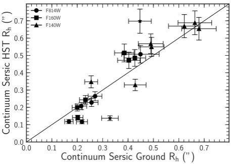
For the 21 galaxies withHST imaging we measure Rh in both ground andHST based photometry, both paramet-rically (Figure2) and non-parametrically. To test how well we recover the sizes in ground-based measurements alone we compare the ground based continuum half light radii to the HST continuum half light radii, deriving a median ra-tio of <RGh/RHSTh >= 0.97±0.05. Applying the same para-metric fitting procedure to the remaining galaxies we derive
0.0 0.1 0.2 0.3 0.4 0.5 0.6 0.7
Continuum Sersic Ground R
h(”)
0.0 0.1 0.2 0.3 0.4 0.5 0.6 0.7
Continuum
Sersic
HST
R
h(”)
[image:6.595.310.539.102.264.2]F814W F160W F140W
Figure 2.The half-light radius derived from S´ersic function fits to both ground based andHST data in Near-IR bands, for 21 galaxies in our sample. Marker shape represents theHST filter, star points indicate galaxies where ground andHST photometry show different morphological features or defects. The majority of sizes show good agreement with <RG
h/RHSTh >=0.97 ± 0.05, independent of the band of the observation.
half-light radii for all 34 galaxies with< Rh>= 000.43±000.06, which equates to 3.55±0.50 kpc at z= 2.22 (the median redshift of the sample). Numerically we derive a median of < Rh>= 000.55±000.04 (4.78±0.41 kpc at the z=2 .22), with<RS´hersic>/RNumericalh >= 0.82±0.04, indicating that the non-parametric fitting procedure broadly reproduces the parametric half-light radii. The median continuum half light size derived for our sample from S´ersic fitting is comparable to that obtained byStott et al.(2013) for HiZELS galaxies out toz= 2.23, with< Rh>= 3.6±0.3 kpc.
We further test the reliability of the recovered sizes (and their uncertainties), by randomly generating 1000 S´ersic models with 0.5< n <2 and 000.1<Rh< 100.0. These mod-els are convolved with the UDS image point spread func-tion and Gaussian random noise is added appropriate for the range in total signal-to-noise for our observations. Each model is then fitted to derive ‘observed’ model parameters. We recover a median size of<RTrueh >/RObsh >= 0.99±0.05 and S´ersic index<nTrue/nObs>= 1.05±0.07. This demon-strates our fitting procedures accurately derives the intrinsic sizes of the galaxies in our sample. From this point forward we take the parametric S´ersic half-light radii as the intrinsic Rhof each galaxy.
As a test of the expected correlation between contin-uum size and the extent of nebular emission (e.g.Bournaud et al. 2008;F¨orster Schreiber et al. 2011a), we calculate the Hα(O[iii] for galaxies atz >3) half light radii of the galax-ies in the sample. We follow the same procedures as the continuum stellar emission, but using narrow band images generated from the integral field data. We model the PSFs, using a stack of unsaturated stars that were observed with the spectrographs at the time of the observations using a multi-component S´ersic (n= 0.5) model.
We derive both parametric and non-parametric half-light radii from S´ersic fitting and numerical analysis within 2Rp. For the full sample of 34 galaxies the median paramet-ric nebula half-light radii is<RNebula
<RS´ersic
h >/RNumericalh >= 0.93±0.04. The nebula emission sizes on average are consistent with the continuum stellar size, with <RContinuum
h >/RNebulah >= 1.15±0.19. We note that the low-surface brightness of the outer regions of the high-redshift galaxies may account for the apparent ∼10% smaller nebula sizes in our sample.
3.3 Galaxy Inclination and Position angles
To derive the inclination of the galaxies in our sample we first measure the ratio of semi–minor (b) and major (a) axis from the parametric S´ersic model. We derive an uncertainty on the axis ratio of each galaxy by bootstrapping the fitting procedure over an array of initial conditions. For galaxies that are disk-like, the axis ratio is related to the inclination by:
cos2(θinc) = b a
2
−q20 1−q2
0
, (2)
whereθinc= 0 represents a face-on galaxy. The value of q0, which accounts for the fact that galaxy disks are not in-finitely thin, depends on galaxy type, but is typically in the range of q0= 0.13 – 0.20 for rotationally supported galax-ies at z∼0 (e.g. Weijmans et al. 2014). We adopt q0= 0.2 to be consistent with other high redshift integral field sur-veys (KROSS; Harrison et al. 2017, KMOS3D; Wisnioski et al. 2015). The full range of axis ratio in the sample is b/a = 0.2 – 0.9 with<b/a>= 0.69±0.04 corresponding to a median inclination for the sample of< θinc>= 48◦±3◦.
3.4 Emission Line Fitting
Next we derive the kinematics, rotational velocity and dis-persion profiles of the galaxies by performing emission line fits to the spectrum in each data cube.
For the Hαand [Nii] doublet (25) sources we fit a triple Gaussian profile to all three emission lines simultaneously, whilst for [Oiii] emitters a single Gaussian profile is used when we model the [Oiii] λ5007 emission line. We do not have significant detections of theλ4959 [Oiii] orλ4862 Hβ
emission line. The fitting procedure uses a five or six pa-rameter model with redshift, velocity dispersion, continuum and emission line amplitude as free parameters. For the Hα
emitting galaxies we also fit the [Nii]/Hαratio, constrained between 0 and 1.5. The FWHM of the emission lines are cou-pled, the wavelength offsets fixed and the flux ratio of the [Nii] doublet ([Nii]λ6583
[Nii]λ6548) fixed at 2.8 (Osterbrock & Ferland
2006). We define the instrumental broadening of the emis-sion lines from the intrinsic width of the OH sky lines in each galaxy’s spectrum, by fitting a single Gaussian profile to the sky line. The instrumental broadening of the OH sky lines in the J, H and K bands are σint= 71 km s−1±2 km s−1, 50 km s−1±5 km s−1 and 39 km s−1±1 km s−1 respectively. The initial parameters for spectral fitting are estimated from spectral fits to the galaxy integrated spectrum summed from a 100.0 aperture centred on the continuum centre of the galaxy.
We fit to the spectrum in 0.0015 × 000.15 (3×3 spax-els) spatial bins, due to the low signal-to-noise in individual spaxels, and impose a signal-to-noise threshold of S/N≥5 to the fitting procedure. If this S/N is not achieved we bin the
spectrum over a larger area until either the S/N threshold is achieved or the binning limit of 000.35 × 000.35 is reached (∼1.5×the typical AO-corrected psf width). In Figure3we show example Hαand [Oiii] intensity, velocity and velocity dispersion for five galaxies in the sample.
3.5 Rotational Velocities
We use the Hαand [Oiii] velocity maps to identify the kine-matic major axis for each galaxy in our sample. We rotated the velocity maps around the continuum centre in 1◦steps, extracting the velocity profile in 0.15 arcsecond wide slits and calculating the maximum velocity gradient along the slit. We bootstrap this process, adding Gaussian noise to each spaxel’s velocities of order the velocity error derived from emission line fitting. The position angle with the great-est bootstrap median velocity gradient was identified as be-ing the major kinematic axis (PAvel), as shown by the blue line in Figure3.
By extracting the velocity profile of the galaxies in our sample about the kinematic major axis, we are assuming the galaxy is an infinitely thin disk with minimal non-circular motions and is kinematically ’well-behaved’. We note how-ever that this may not be true for all galaxies in sample, with some galaxies having significant non-circular motions leading to an underestimate of the rotation velocity and an overestimate of the velocity dispersion in these galaxies.
The accuracy of the velocity profile extracted for each galaxy depends on the accuracy to which the kine-matic major axis is identified. To quantify the impact on the rotation velocity profile of deriving an incorrect kinematic position angle, we extract the rotation pro-files of our galaxies about there broadband semi-major axis as well as there kinematic axis. On average we find minimal variation between VrotBB(r) and VrotKE(r) with
<VrotBB(r)/VrotKE(r)>= 0.94±0.15.
In order to minimise the impact of noise on our mea-surements, we also fit each emission line rotation velocity curve (v) with a combination of an exponential disk (vD) and dark matter halo (vH). We use these models to extrap-olate the data in the outer regions of the galaxies’ velocity field, as opposed to interpreting the implications of the indi-vidual model parameters. For the disk dynamics we assume that the baryonic surface mass density follows an exponen-tial profile (Freeman 1970) and the halo term can be mod-elled as a modified Navarro, Frenk & White (NFW) profile (Navarro et al. 1997). The halo velocity model converges to the NFW profile at large distances and, for suitable values ofr0, it can mimic the NFW or an isothermal profile over the limited region of the galaxy which is mapped by the ro-tation curve. The dynamics of the galaxy are described by the following disk and halo velocity components:
v2=vD2 +v
2
H,
vD2(x) =
1 2
GMd
Rd
(3.2x)2(I0K0I1K1),
vH2(r) =
6.4Gρ0r03
r
ln(1 + r
r0
)−tan−1(r
r0 ) +1
2ln[1 + (
r r0
)2]
,
HST
WFC3 F140W 0.25"H
0.25"V
rot
Quality 2V
mod
rms: 21.0obs
12 8 4 0 4 8 12
50
0
50
Ve
l.
(k
m
s
1
)
z~2.24
SHIZELS21
0.00 7.64e01 54.9 72.9 47.3 206.5
HST
WFC3 F140W 0.25"H
0.25"V
rot
Quality 3V
mod
rms: 26.0obs
8 4 0 4 8
50
0
50
Ve
l.
(k
m
s
1
)
z~1.45
SHIZELS10
0.00 8.78e01 53.8 48.5 5.0 155.3
UKIDSS
Kband 0.25"H
0.25"V
rot
Quality 2V
mod
rms: 20.0obs
8 4 0 4 8
100
50
0
50
100
Ve
l.
(k
m
s
1
)
z~2.24
SHIZELS23
0.00 5.09e01 86.5 31.7 2.5 211.2
HST
WFC3 F140W 0.25"H
0.25"V
rot
Quality 2V
mod
rms: 16.0obs
4 0
4
50
0
50
Ve
l.
(k
m
s
1
)
z~2.22
SHIZELS2
0.00 1.09e+00 62.8 57.3 28.8 137.1
HST
WFC3 F160W 0.25"H
0.25"V
rot
Quality 2V
mod
rms: 29.0obs
8
4 0
4
8
Radius (kpc)
100
50
0
50
100
Ve
l.
(k
m
s
1
)
z~1.49
SHIZELS19
[image:8.595.46.533.99.517.2]0.00 4.74e01 62.3 139.5 6.4 254.8
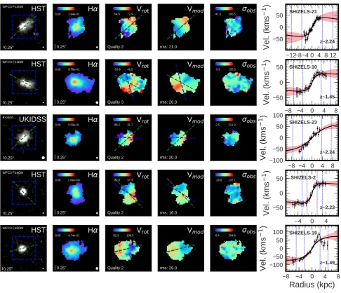
Figure 3.Example of spatially resolved galaxies in our sample. From left to right; Broadband photometry of the galaxy (left), with PAim (green dashed line) and data cube field of view (blue dashed square). Hαor [Oiii] flux map, velocity map, velocity model and
velocity dispersion map, derived from the emission line fitting. PAvel(blue dashed line) and PAim(green dashed line) axes plotted on the velocity map and model. Rotation curve extracted about kinematic position axis (right). Rotation curve shows lines of Rhand 2Rh derived from S´ersic fitting, as well 1σerror region (red) of rotation curve fit (black line).
mass and disk scale length respectively. In fitting this model to the rotation profiles, there are strong degeneracies be-tween Rd, ρ0 andr0. To derive a physically motivated fit, we modified the dynamical model to be a function of the dark matter fraction, disk scale radius and disk mass. Using the stellar mass, derived in Section3, as a starting parame-ter for the disk mass, enables the fitting routine to converge. The dynamical centre of the galaxy was allowed to vary in the fitting procedure by having velocity and radial offsets as free parameters constrained to ±20 km s−1 and ±0.1 arc-seconds. The dark matter fraction in galaxy with a given disk and dark matter mass is given by:
fDM=
MDM
Md+MDM
,
where the dark matter mass and disk mass are derived from;
MDM(<R) =
Z R
0
ρ(r)4πr2dr=
Z R
0
4πρ0r30r2 (R+r0)(R2+r2
0)
dr,
Md(<R) =
Z R
0
e−
r Rd2πrdr,
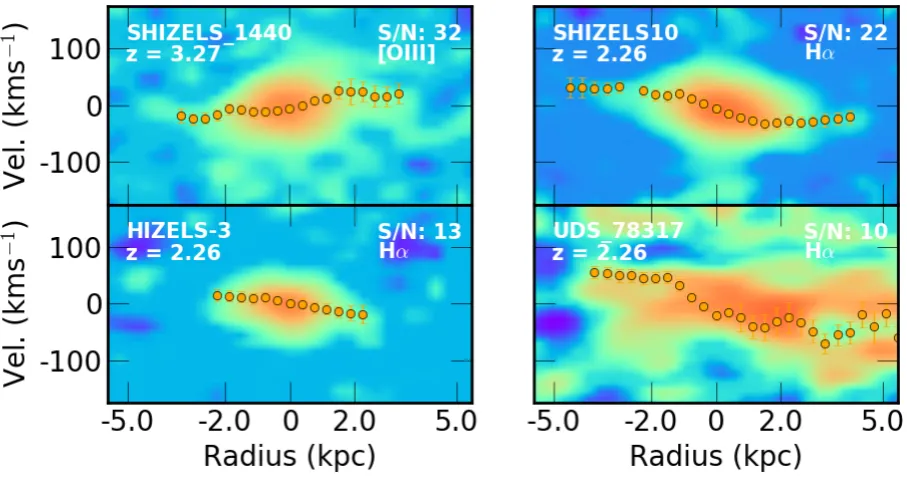
Figure 4.The position-velocity diagrams of four galaxies in the sample extracted from a slit about the kinematic major axis of each galaxy. The galaxies shown are selected from bins of emission line S/N derived from the galaxies integrated spectrum. We overlay each galaxies ionised gas rotation curve as derived in Section 3.4for comparison. Redshift, emission line and S/N of each position-velocity map is shown, with upper left to bottom right as high to low galaxy integrated S/N.
model. The 1σ error is defined as the region in parameter space where theδχ2 =|χ2best-χ2params| ≤number of param-eters. Prior to themcmcprocedure we apply the radial and velocity offsets to the rotation to reduce the number of free parameters and centre the profiles. The parameter space for 1σ uncertainty is thusδχ2≤3. Taking the extremal veloc-ities derived within the δχ2≤3 parameter space provides the uncertainty on Vrot. The rotation velocities and best fit dynamical models are shown in Figure 3. The full samples kinematics are shown in Appendix D. To show the full ex-tent of the quality of data in our sample, we derive position-velocity diagrams for each galaxy. In Figure4we show one position-velocity diagram from each quartile of galaxy inte-grated signal to noise with the galaxies ionised gas rotation curve overlaid.
Next we measure the rotation velocities of our sam-ple at 2Rh (= 3.4 Rd for an exponential disk) (e.g. Miller et al. 2011). For each galaxy we convolve Rh with the PSF of the IFU observation and extract velocities from the ro-tation curve. At a given radii our measurement is a me-dian of the absolute values from the low and high com-ponents of the rotation curve. Finally we correct for the inclination of the galaxy, as measured in Section 3.2. On average the extraction of Vrot2Rh from each galaxy’s rota-tion curve requires extrapolarota-tion from the last data point (Rlast) to 2Rh in our sample, where the median ratio is
<Rlast/2Rh>= 0.42±0.04. However for the sample, the average Vrot2Rh is ∼14% smaller than the velocity of the
last data point (Vlast) with<Vlast/Vrot2Rh>= 1.14±0.11 which is within 1σ. Figure5shows the distribution of radial and velocity ratios.
To quantify the impact of beam smearing on the
ro-tational velocity measurements, we follow the methods of
Johnson et al.(2018), and derive a median ratio of<Rd/ RPSFh
>= 2.17±0.18 which equates to an average rotational ve-locity correction of 1 %. We derive the correction for each galaxy in the sample and correct for beam smearing effects. AppendixCTableC1displays the inclination, beam smear-ing corrected rotation velocity (Vrot2Rh) for each galaxy.
The full distribution of Rd/ RPSF
h is shown in Appendix E. The median inclination beam smearing corrected rota-tion velocity in our is sample is<Vrot2Rh>= 64±14 km s−1, with the sample covering a range of velocities from Vrot2Rh= 17 – 380 km s−1. The SINS/ZC-SINF AO survey (Schreiber et al. 2018) of 35 star forming galaxies at z∼2 identify a median rotation velocity of<Vrot>= 181 km s−1, with a range of Vrot= 38 – 264 km s−1. This approximately a factor of three larger than our sample, although we note their sample selects galaxies of higher stellar mass with log(M∗[M]) = 9.3 – 11.5 whereas our selection selects lower mass galaxies.
3.6 Kinematic Alignment
The angle of the galaxy on the sky can be defined as the morphological position angle (PAim) or the kinematic posi-tion angle (PAvel). High-redshift IFU studies (e.g.Wisnioski et al. 2015;Harrison et al. 2017) use the misalignment be-tween the two position angles to provide a measure of the kinematic state of the galaxy. The (mis)alignment is defined such that:
Figure 5.Left:Histogram of the ratio of the last rotational velocity data point to the velocity at 2Rh.Right:Histogram of the ratio of the radius of the last data point on rotation curve to 2Rh. Inset histograms show the distribution for the kinematic sub-classes (Section 3.10). Dashed line indicates the median in both figures, where <Rlast/2Rh>= 0.42±0.04 and <Vlast/Vrot2Rh >= 1.14±0.11. On average extracting the rotational velocity at 2Rhrequires extrapolation of the model beyond the last data point, leading to an decrease in velocity of∼14%.
where Ψ takes values between 0◦ and 90◦. In Figure6 we show Ψ as a function of image axis ratio for the sample compared to the KROSS survey of∼700 star-forming galax-ies at z∼0.8. The sample covers a range of position an-gle misalignment, with<Ψ>=31.8◦±5.7◦, 10.52◦±19.8◦, 33.2◦±15.2◦ & 21.8◦±17.5◦at z= 0.84, 1.47, 2.22 & 3.33 respectively. This is larger than that identified in KROSS atz∼0.8 (13◦), but at all redshifts comparable to or within the criteria of Ψ≤30◦
imposed byWisnioski et al.(2015), to define a galaxy as kinematically ‘disky’. This indicates the average galaxy in our sample is on the boundary of what is considered to be a disk. A summary of the morphologi-cal properties for our sample is shown in AppendixCTable
C1. Example broadband images of our sample are shown in the left panel of Figure 3, with the appropriate PAim and integral field spectrograph field of view. The kinematic PA for the sample is derived in Section3.4. We will use this cri-teria, together with other dynamical criteria later to define the most disk-like systems.
3.7 Two-dimensional Dynamical Modelling
To provide a parametric derivation and test of the numerical kinematic properties derived for each galaxy, we model the broadband continuum image and two-dimensional velocity field with a disk and halo model. The model is parametrised in the same way as the one-dimensional kinematic model used to interpolate the data points in each galaxies’ rota-tion curve (Secrota-tion3.5) but takes advantage of the full two-dimensional extent of the galaxies velocity field. To fit the dynamical models to the observed images and velocity fields, we again use anMCMCalgorithm. We first use the imaging data to estimate the size, position angle and inclination of the galaxy disk. Then using the best-fit parameter values from imaging as a first set of prior inputs to the code, we simultaneously fit the imaging and velocity fields. We allow
the dynamical centre of the disk and position angle (PAvel) to vary, but require that the imaging and dynamical cen-tre to lie within 1 kpc (approximately the radius of a bulge atz∼1;Bruce et al. 2014). We note also that we allow the morphological and dynamical major axes to be independent. The routine converges when no further improvement in the reduced chi-squared of the fit can be achieved within 30 it-erations. For a discussion of the model and fitting procedure seeSwinbank et al.(2017).
For the sample of 34 galaxies the average of the ratio of kinematic positional angle derived from the velocity map to numerical modelling is
<PAvel(Slit)/PAvel(2D)>=0.97±0.09. Whilst the mor-phological position angle agree on average with
<PAim(S´ersic)/PAim(2D)>=1.10±0.14. We compare the velocity field generated from the fitting procedure, (see Figure3for examples), to the observed field for each galaxy derived from emission line fitting (Section 3.4). We derive a velocity error weighted rms based on the residual for each galaxy, and normalise this by the galaxies rotational velocity (Vrot2Rh). On average the sample is well described by the disk and halo model, with the median rms of the residual images being<rms>=22±1.42
3.8 Velocity Dispersions
To further classify the galaxy dynamics of our sources we also make measurements of the velocity dispersion of the star-forming gas (σ0). High redshift star forming galaxies are typically highly turbulent clumpy systems, with non-uniform velocity dispersions (e.g.Genzel et al. 2006;Kassin et al. 2007;Stark et al. 2008;F¨orster Schreiber et al. 2009b;
Figure 6.The absolute misalignment between the kinematic and morphological axes (Ψ) as a function of minor(b) to semi-major(a) axis ratio for the galaxies in our sample derived from S´ersic fitting as a function of. Our sample is coloured by red-shift as Figure 1, and the KMOS Redshift One Spectroscopic Survey (KROSS) is shown for comparison as the grey shaded region. The circles indicate galaxies with Vrot2Rh/σmedian>1 whilsttriangleshighlight galaxies with Vrot2Rh/σmedian<1. The majority of galaxies in our sample are moderately inclined with <b/a>=0.68±0.04 showing kinematic misalignment of Ψ<48◦.
of each galaxy by taking the median of each velocity disper-sion map, examples of which are shown in Figure 3, in an annulus between Rh and 2Rh. This minimises the effects of beam smearing towards the centre of the galaxy as well as the impact of low surface brightness regions in the outskirts of the galaxy. We also measure the velocity dispersion from the inner regions of the dispersion map as well as the map as a whole, finding excellent between all three quantities, to within on average 3%.
To take into account the impact of beam smearing on the velocity dispersion of the galaxies in our sample we fol-low the methods of Johnson et al.(2018). We measure the ratio of galaxy stellar continuum disk size (Rd) to the half-light radii of the PSF of the AO observations deriving a median ratio of <Rd/ RPSFh >= 2.17±0.18 which equates to an average velocity dispersion correction of∼4%. We de-rive the correction for each galaxy in the sample and correct for beam smearing effects.
The average velocity dispersion for our sample is
< σmedian>= 85±6 km s−1, with full range ofσmedian= 40 – 314 km s−1. This is similar to KROSS at z∼1 which has < σmedian>= 83±2 km s−1 but much higher than the KMOS3D survey which identified a decrease in the in-trinsic velocity dispersion of star-forming galaxies by a factor of two from 50 km s−1 at z∼2.3 to 25 km s−1 at z∼0.9 (Wisnioski et al. 2015). The evolution of ve-locity dispersion with cosmic time is minimal in our sample with < σmedian>= 79±15 km s−1, 87±10 km s−1, 79±12 km s−1 & 83±27 km s−1 at z= 0.84, 1.47, 2.23 & 3.33 respectively. The KMOS Deep Survey (Turner et al. 2017) identified a stronger evolution in velocity dispersion withσint= 10 - 20 km s−1atz∼0, 30 - 60 km s−1atz∼1 and 40 - 90 km s−1 at z∼3 in star-forming galaxies. This indi-cates that the lower redshift galaxies in our sample are more
turbulent than the galaxy samples discussed inTurner et al.
(2017). We note however, that the different selection func-tions of the observafunc-tions will influence this result.
To measure whether the galaxies in our sample are ‘dis-persion dominated’ or ‘rotation dominated’ we take the ratio of rotation velocity (Vrot2Rh) to intrinsic velocity
disper-sion (σmedian), followingWeiner et al.(2006);Genzel et al.
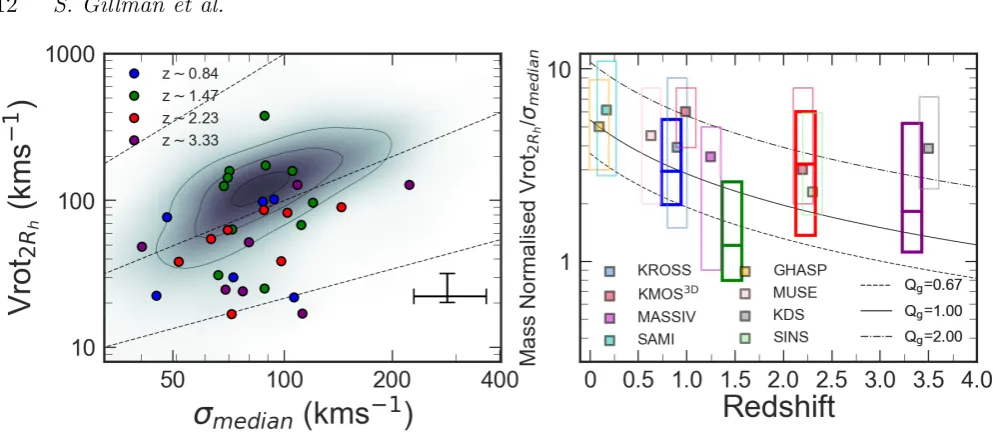
(2006). Taking the full sample of 34 galaxies, we find a me-dian ratio of rotational velocity to velocity dispersion, across all redshift slices of <Vrot2Rh/σmedian>= 0.82±0.13 with ∼32% having Vrot2Rh/σmedian>1 (Figure 7). This is sig-nificantly lower than other high redshift IFU studies such as KROSS, in which 81% of its ∼600 star forming galax-ies having Vrot2Rh/σ0>1 with a<Vrot2Rh/σ0>= 2.5±1.4.
We note that the median redshift of the KROSS sample is
< z >= 0.8, compared to< z >= 2.22 for our sample. John-son et al. (2018) identified that galaxies of stellar mass 1010Mshow a decrease in Vrot2Rh/σ0 fromz∼0 toz∼2 by a factor∼4.
The SINS/ZC-SINF AO survey of 35 star forming galaxies at z∼2 identify a median Vtot/σ0= 3.2 ranging from Vtot/σ0= 0.97 – 13 (Schreiber et al. 2018). In our sample at z= 0.84, 1.47, 2.23 & 3.33 the medain ratio is
<Vrot2Rh/σmedian>= 1.26±0.43, 1.75±0.90, 1.03±0.20
& 0.52±0.22 respectively. This indicates that on average the dynamics of thez∼3.33 galaxies in our sample are more dispersion driven.Turner et al.(2017) identified a similar re-sult with KMOS Deep Survey galaxies atz∼3.5, finding a median value of VC/σint= 0.97±0.14.
In order to compare our sample directly to other star-forming galaxy surveys we must remove the inherent scaling between stellar mass and V/σ, by mass normalising each comparison sample to a consistent stellar mass, for which we use M∗= 1010.5M, following the procedures ofJohnson
et al.(2018). In Figure7we show the mass normalised V/σ
of our sample as a function of redshift as well eight compari-son samples taken from the literature. GHASP (Epinat et al. 2010;z= 0.09), SAMI (Bryant et al. 2015;z= 0.17), MAS-SIV (Epinat et al. 2012;z= 1.25), KROSS (Stott et al. 2016;
z= 0.90), KMOS3D (Wisnioski et al. 2015; z= 1 & 2.20) SINS (Cresci et al. 2009;z= 2.30) and KDS (Turner et al. 2017; z= 3.50). We overplot tracks of Vrot2Rh/σmedian as function of redshift, for different Toomre disk stability crite-rion (Qg;Toomre 1964) following the procedures ofJohnson et al.(2018) andTurner et al.(2017), normalised to the me-dian V/σ of the GHASP Survey atz= 0.093. The galaxies in our sample align well with the mass normalised compar-ison samples from the literature, with a trend of increasing V/σ with increasing cosmic time, as star-forming galaxies become more rotationally dominated.
3.9 Circular Velocities
It is well known that high redshift galaxies are highly turbu-lent systems with heightened velocity dispersions in compar-ison to galaxies in the local Universe. (e.g.F¨orster Schreiber et al. 2006,2009b;Genzel et al. 2011;Swinbank et al. 2012a;
Figure 7.Left: Distribution of velocity Vrot2Rhandσmedianin our sample, coloured by spectroscopic redshift as in Figure1. The KROSS
z∼0.8 survey is shown for comparison by the shaded region. Lines of 1.5Vrot/σmedian, Vrot/σmedianand Vrot/1.5σmedian shown for reference.Right: Mass normalised Vrot2Rh/σmedianas function of redshift, the 16th and 84th percentile shown by the extent of the box, median as a solid line at each redshift. We also show eight comparison surveys of star-forming galaxies from 0.09< z <3.5 selected from the literature with median values shown by the squares. We plot tracks of Vrot2Rh/σmedianas function of redshift, for different Toomre disk stability criterion (Qg;Toomre 1964) following the procedures ofJohnson et al.(2018). The majority of the sample has a mass normalised Vrot2Rh/σmedian>1, with an indication of a slight evolution in the dominate dynamical support process with cosmic time, with Vrot2Rh/σmedianincreasing at lower redshift.
constant velocity dispersion, the true circular velocity of a galaxy (Vcirc(r)) is given by
V2circ(r) = V2rot(r) + 2σ02( r
Rd), (4)
where Rd is the disk scale length and σ0 is the intrin-sic velocity dispersion of the galaxy. For a galaxy with Vrot/σ0≥3 the contribution from turbulent motions is neg-ligible and Vcirc(r)≈Vrot(r). All the galaxies in our sample have Vrot/σ0<3. For each object we convert the inclina-tion corrected rotainclina-tional velocity profile to a circular veloc-ity profile. Following the same methods used to derive the rotational velocity of a galaxy (Section 3.5), we fit one di-mensional dynamical models to the circular velocity profiles of each galaxy and extract the velocity at two times the stel-lar continuum half light radii of the galaxy (Vcirc(r = 2Rh)). The ratio of Vcirc(r = 2Rh) to Vrot(r = 2Rh) for each galaxy is shown in AppendixCTableC1. The median circular ve-locity to rotational veve-locity ratio for galaxies in our sample is
<Vcirc(r = 2Rh)/Vrot(r = 2Rh)>= 3.15±0.41 ranging from Vcirc(r = 2Rh)/Vrot(r = 2Rh) = 1.17 – 12.91.
3.10 Sample Quality
Our sample of 34 star forming galaxies covers a broad range in rotation velocity and velocity dispersion. Figure 3 and Figure 7 demonstrate there is dynamical variance at each redshift slice, with a number of galaxies demonstrating more dispersion driven kinematics. To constrain the effects of these galaxies on our analysis, we define a sub–sample of galaxies with high signal to noise, rotation dominated kine-matics and ‘disky’ morphologies.
We note that if we were to split the sample by galaxy in-tegrated signal-to-noise rather than morpho-kinematic prop-erties, we would not select ‘disky’ galaxies with rotation dominated kinematics as the best quality objects. Splitting the sample into three bins of signal to noise with S/N≤14 (low), S/N>14 & S/N≤23 (medium) and S/N>24 (high) we find 12, 11 and 11 galaxies in each bin respectively with the low and median S/N bins having a median redshift of
z= 1.47±0.17 and 1.45±0.54 whilst the highest S/N bin has a median redshift ofz= 2.24±0.38. All three signal to noise bins and have median rotation velocities, velocity dis-persion and specific angular momentum values within 1σof each other, therefore not distinguishing between ‘disky’ ro-tation dominated galaxies and those with more dispersion driven dynamics.
The morpho-kinematic criteria that define our three sub–samples are;
• Quality 1: Vrot2Rh/σmedian>1 and ∆PAim,velΨ<30 ◦
• Quality 2: Vrot2Rh/σmedian>1 or ∆PAim,velΨ<30◦
• Quality 3: Vrot2Rh/σmedian<1 and ∆PAim,velΨ>30◦
Of the 34 galaxies in the sample, 11 galaxies have Vrot2Rh/σmed>1 and 17 have ∆PAim,velΨ<30◦. We clas-sify 6 galaxies that pass both criteria as ‘Quality 1’ whilst galaxies that pass either criteria are labelled ‘Quality 2’ (17 galaxies). The remaining 11 galaxies that do not pass either criteria are labelled ‘Quality 3’.
Figure 8. Rotation velocity extracted from the rotation curve at 2Rh as a function of stellar mass derived from SED fitting as described in Section 3, formally known as the Stellar Mass Tully Fisher relation. The sample is coloured by spectroscopic red-shift, as in Figure1, whilst the blue shaded region represents the KROSSz∼1 sample (Harrison et al.(2017)). Thestarsrepresent ‘Quality 1’ targets (Vrot2Rh/σmed>1 and ∆PAim,velΨ<30
◦),
circles ‘Quality 2’ (Vrot2Rh/σmed>1 or ∆PAim,velΨ<30 ◦) and triangles ‘Quality 3’ galaxies (Vrot2Rh/σmed<1 and ∆PAim,velΨ>30◦). We also showz∼0 tracks fromReyes et al. (2011), z∼3.5 tracks for rotation dominated (Vrot2Rh/σint>1) and dispersion dominated (Vrot2Rh/σint<1) galaxies in the KMOS Deep Survey (KDS) fromTurner et al.(2017). There is a clear distinction between the different sub–samples, with ‘Quality 1’ galaxies having higher rotation velocity for a given stellar mass, aligning with the KROSS sample. ‘Quality 3’ targets have lower rotation velocities, aligning more with Vrot2Rh/σint<1 KMOS Deep Surveyz∼3.5 track, whilst ‘Quality 2’ targets on average lie in between, with intermediate rotation velocities for a given stellar mass. The median uncertainty on rotational velocity at each redshift is shown in the lower left corner as well as the un-certainty of the stellar mass. Thez∼1.47 ‘Quality 3’ galaxy, with Vrot2Rh∼380 km s
−1 has low inclination of ∼25◦, hence large line-of-sight velocity correction.
the full sample as well the sub–samples, indicating the more turbulent galaxies in our sample do not bias our interpreta-tions of the data. In each of the following secinterpreta-tions we remark on the properties on ‘Quality 1 ’ and ‘Quality 2’ galaxies.
3.11 Rotational velocity versus stellar mass
The stellar mass ‘Tully-Fisher relationship’, (Figure 8), represents the correlation between the rotational velocity (Vrot2Rh) and the stellar mass (M∗) of a galaxy (TFR;
Tully & Fisher 1977, Bell & de Jong 2001). The relation-ship demonstrates the link between total mass (or ‘dynami-cal mass’)2of a galaxy, which can be probed by how rapidly the stars and gas are rotating, and the luminous (i.e. stellar) mass.
In Figure 8 we plot Vrot2Rh as a function of stellar mass for our sample as well as a sample of z <0.1 star-forming galaxies from Reyes et al. (2011) using spatially-resolved Hα kinematics. The KROSS survey at z∼1 is
2 For rotationally-dominated galaxiesTiley et al.(2018)
also indicated (Harrison et al. 2017). We over plot two tracks from the KMOS Deep Survey (KDS; Turner et al. 2017), with median redshift of z∼3.5. The KDS sample is split into ‘rotation-dominated’ systems (Vrot2Rh/σint>1) and ‘dispersion-dominated’ systems (Vrot2Rh/σint<1), for which we show both tracks.
Figure 8 shows a distinction between ‘Quality 1’ and ‘Quality 2 / 3’ galaxies. ‘Quality 1’ galax-ies, which have the most disk-like properties have higher rotation velocity for a given stellar mass with a <Vrot2Rh>= 151 km s−1±13 km s−1, and align with the rotational velocities of the KROSS sample. The median rotation velocity of ‘Quality 2 & 3’ galax-ies is <V2Rh>= 53 km s−1±10 km s−1, occupying sim-ilar parameter space to the Vrot2Rh/σint<1 KMOS
Deep Survey z∼3.5 track. This is a consequence of construction, as ‘Quality 1’ galaxies have a median
<Vrot2Rh/σmed>= 1.74±0.30 whilst ’Quality 2 & 3’ sources have<Vrot2Rh/σmed>= 0.62±0.11
The Tully-Fisher relation provides a method to con-strain galaxy dynamical masses however due to degeneracies and ambiguity in the evolution of the intercept and slope of the relationship with cosmic time (e.g.Ubler et al. 2017¨ ; Ti-ley et al. 2018), and the strong implications of sample selec-tion this becomes increasingly challenging. There is discrep-ancy amongst other high redshift star-forming galaxy stud-ies (e.g.Conselice et al. 2005;Flores et al. 2006;Di Teodoro et al. 2016;Pelliccia et al. 2017) finding no evolution in the intercept or slope of Tully-Fisher relation. Even with the inclusion of non-circular motions through gas velocity dis-persions via the kinematic estimator S0.5 (e.g.Kassin et al.
2007; Gnerucci et al. 2011) no evolution across ∼8Gyr of cosmic time is found. Whilst other studies (e.g.Miller et al. 2012; Sobral et al. 2013b) identify evolution in the stellar mass zero point of ∆M∗= 0.02±0.02 dex out toz= 1.7.
We have demonstrated that the galaxies in our sample exhibit properties that are typical for ‘main sequence’ star forming galaxies fromz= 0.8 – 3.5 and show good agreement with other high-redshift integral-field surveys when the sam-ple selection is well matched (e.g.Ubler et al. 2017¨ ;Harrison et al. 2017; Turner et al. 2017). For the remainder of this work we focus on a fundamental property of the galaxies in our sample; their angular momentum, which incorporates the observed velocity, galaxy size and stellar mass.
4 ANGULAR MOMENTUM
With a circular velocity, stellar mass and size derived for each galaxy, we can now turn our attention to analysing the angular momentum properties of our sample. First we investigate the galaxy stellar specific angular momentum of the disk. We then take advantage of the high resolution of the data, and study the distribution of angular momentum within each galaxy.
4.1 Total Angular Momentum
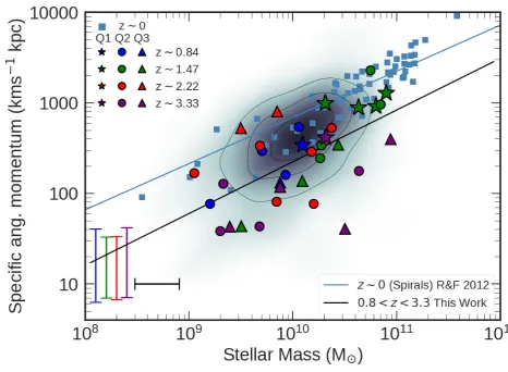
Figure 9.Specific stellar angular momentum as measured at 2Rh as a function of stellar mass. The sample coloured by spectroscopic redshift as as shown in Figure1, and the blue shaded regions represents the KROSS z∼1 sample (Harrison et al. 2017). The stars
represent ‘Quality 1’ targets (Vrot2Rh/σmed>1 and ∆PAim,velΨ<30
◦), circles ‘Quality 2’ (Vrot
2Rh/σmed>1 or ∆PAim,velΨ<30 ◦) andtriangles‘Quality 3’ galaxies (Vrot2Rh/σmed<1 and ∆PAim,velΨ>30
◦). Thez∼0Romanowsky & Fall(2012) comparison sample is shown, with the fit to the data of the form log10(j∗) =α+β(log10(M∗/M)−10.10), withα= 2.89 andβ= 0.51, whilst for KROSS (z∼1)α= 2.58 and β= 0.62. Our sample appears in good agreement with other z∼1 samples, having lower specific stellar angular momentum for a given stellar mass than galaxies atz∼0, with aα= 2.41 and β= 0.56. The median uncertainty on specific angular momentum at each redshift is shown in the lower left corner as well as the uncertainty of the stellar mass.
and circular velocity, comprises of three uncorrelated vari-ables with a mass scale and a length scale times a rotation-velocity scale (Fall & Efstathiou 1980,Fall 1983). The stellar specific angular momentum also removes the inherent scal-ing between total angular momentum and mass. It is derived from:
j∗= J∗ M∗
=
R
(rׯv(r))ρ∗(r)d3r R
ρ∗(r)d3r
, (5)
where r and ¯v are the position and mean-velocity vectors (with respect to the centre of mass of the galaxy) andρ(r) is the three dimensional density of the stars and gas ( Ro-manowsky & Fall 2012).
In order to compare between observations and empiri-cal models (or numeriempiri-cal models, as we will in Section4.2.2), this expression can be simplified to be a function of intrinsic circular rotation velocity of the star forming gas and the stel-lar continuum half light radius. These intrinsic properties of the galaxy are correlated to the observable rotation velocity
and disc scale length by the inclination of the galaxy and the PSF of the observations. As derived byRomanowsky & Fall(2012), this expression can be expanded to incorporate non-exponential disks. The specific angular momentum can be written as function of inclination and S´ersic index3:
j∗=knCivsRh, (6)
Wherevs is the rotation velocity at 2×the half-light radii (Rh), Ciis the correction factor for inclination, assumed to
be sin−1(θinc) (see Appendix A ofRomanowsky & Fall 2012)
and knis a numerical coefficient that depends on the S´ersic
index,n, of the galaxy and is approximated as:
kn= 1.15 + 0.029n+ 0.062n2, (7)
We derive the specific stellar angular momentum of all 34
![Figure 1. Left: The Hα and [Oiii] dust-corrected star formation rate of each galaxy as function of stellar mass derived deriving frommagphys](https://thumb-us.123doks.com/thumbv2/123dok_us/9303137.430620/4.595.49.526.88.297/figure-corrected-formation-function-stellar-derived-deriving-frommagphys.webp)