Accepted Manuscript
Optimized Projection for Hashing
Chaoqun Chu, Dahan Gong, Kai Chen, Yuchen Guo, Jungong Han,
Guiguang Ding
PII:
S0167-8655(18)30147-8
DOI:
10.1016/j.patrec.2018.04.027
Reference:
PATREC 7155
To appear in:
Pattern Recognition Letters
Received date:
26 January 2018
Revised date:
28 March 2018
Accepted date:
17 April 2018
Please cite this article as: Chaoqun Chu, Dahan Gong, Kai Chen, Yuchen Guo, Jungong Han,
Guiguang Ding, Optimized Projection for Hashing,
Pattern Recognition Letters
(2018), doi:
10.1016/j.patrec.2018.04.027
ACCEPTED MANUSCRIPT
Highlights
• A novel unified formulation for Hashing learning is put forward that overall performance can be optimized.
• We give a general framework for OPH such that it can be incorporated with different Hashing methods.
• For the orthogonality-constrained problem of OPH, we put forward an effective learning algorithm.
ACCEPTED MANUSCRIPT
Pattern Recognition Letters
journal homepage: www.elsevier.com
Optimized Projection for Hashing
ChaoqunChua, DahanGonga, KaiChena, YuchenGuoa, JungongHanb, GuiguangDinga,∗∗
aSchool of Software, Tsinghua University, Beijing 100084, China
bSchool of Computing and Communications, Lancaster University, Lancaster, LA1 4YW, UK
ABSTRACT
Hashing, which seeks for binary codes to represent data, has drawn increasing research interest in recent years. Most existing Hashing methods follow a projection-quantization framework which first
projectshigh-dimensional data into compact low-dimensional space and thenquantifiesthe compact data into binary codes. The projection step plays a key role in Hashing and academia has paid con-siderable attention to it. Previous works have proven that a good projection should simultaneously 1) preserve important information in original data, and 2) lead to compact representation with low quan-tization error. However, they adopted a greedy two-step strategy to consider the above two properties
separately. In this paper, we empirically show that such a two-step strategy will result in a sub-optimal solution because the optimal solution to 1) limits the feasible set for the solution to 2). We put forward a novel projection learning method for Hashing, dubbedOptimized Projection(OPH). Specifically, we propose to learn the projection in a unified formulation which can find a goodtrade-off such that theoverallperformance can be optimized. A general framework is given such that OPH can be incor-porated with different Hashing methods for different situations. We also introduce an effective
gradi-ent-based optimization algorithm for OPH. We carried out extensive experiments for Hashing-based Approximate Nearest Neighbor search and Content-based Data Retrieval on six benchmark datasets. The results show that OPH significantly outperforms several state-of-the-art related Hashing methods.
c
2018 Elsevier Ltd. All rights reserved.
1. Introduction
The demand for effective indexing structures emerged
re-cently which can perform Approximate Nearest Neighbor (ANN) search efficiently given a large-scale database. One of
the best known structures is tree (Friedman et al., 1977) provid-ing logarithmic searchprovid-ing complexity. But tree-based structure may reduce to exhaustive linear search given high-dimensional data (Gionis et al., 1999) which is more common in real world. Hashing, which represents data by binary codes, can effectively
cope with such problem. For example, we just need about 1GB memory to load 32 million points with each point represented by 256 bits and performing ANN search needs less than 1 sec-ond as only simple bit operations are required to compute Ham-ming distance (He et al., 2013). Due to its low storage cost and very high retrieval efficiency, in recent decade Hashing has
drawn increasing interest from both academia and industry.
∗∗Corresponding author: Tel.:+86-010-62773280; fax:+86-010-62773281;
e-mail:[email protected](Guiguang Ding)
Locality Sensitive Hashing (LSH) (Andoni and Indyk, 2006) is one of the most celebrated models. It adopts random linear projections to map original feature vector to binary codes. Such coding method is quite fast. But in practice, long Hashcodes are required to achieve satisfactory performance because it is data-independent (Zhang et al., 2010). To tackle this problem, sev-eral machine learning techniques have been adopted to design effective and compact Hashcodes, such as Principle
Compo-nents Analysis, Manifold Learning, Semi-supervised Learning, and Restricted Boltzmann Machine, which respectively lead to PCA Hashing (Jegou et al., 2010), Spectral Hashing (Weiss et al., 2008), and Semi-supervised Hashing (Wang et al., 2010). Such deta-dependent Hashing methods can exploit important information hidden in the original features, like global Eu-clidean distance, local manifold structure, and etc.
ACCEPTED MANUSCRIPT
0.71 -0.33 -0.51 0.44 0.47 -0.51 -0.42 0.64 -0.82 0.67 0.39 -0.55 -0.36 0.17 0.54 -0.53
0.57 -0.10 -0.03 0.33 -0.23 -0.22 -0.31 0.01
1 -1 -1 1 -1 -1 -1 1
1 1 -1 1 -1 -1 -1 -1 0.44 0.20
-0.12 0.24 -0.31 -0.09 -0.19 -0.15
Quantization
Quantization Re-projection Projection
Original Features
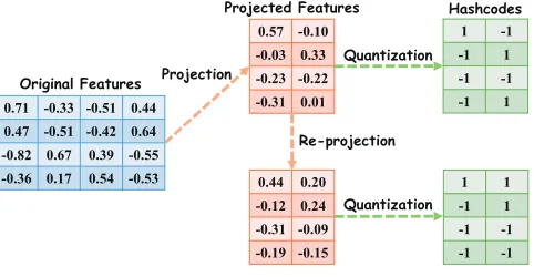
[image:4.595.38.279.64.189.2]Projected Features Hashcodes
Fig. 1. The flowchart of Hashing. Up) The projection-quantization frame-work. Down) An extra re-projection is adopted for better result.
(high-dimensional) original features are projected into a low-dimensional compact space whose low-dimensionality is always equal to the target Hashcode length by a real-value projection function. Secondly, the real-value compact representation is quantified into binary codes by, in most cases, thresholding. A flowchart of such framework is illustrated in Figure 1 Up. De-spite the recent emerging research on quantization (He et al., 2013; Kong and Li, 2012a; Liu et al., 2017a; Shen et al., 2018; Guo et al., 2018), most researchers have paid and are paying more attention to the projection step (Chen et al., 2014; Jegou et al., 2010; Kumar and Udupa, 2011; Wang et al., 2010; Weiss et al., 2008; Zhang et al., 2011; Liu et al., 2015) because this lays the foundation for Hashing and more effective projection
can always lead to better result (Gong and Lazebnik, 2011). Observed from literatures, an effective projection should
sat-isfy the following properties simultaneously: 1) preserving im-portant information in original features, such as global Eu-clidean (Jegou et al., 2010), local manifold structure (Liu et al., 2011; Weiss et al., 2008), or pair-wise label information (Wang et al., 2010; Guo et al., 2017a; Liu et al., 2017b), etc; and 2) leading to projected data with low quantization error which oc-curs when mapping real-value features to binary codes (Gong and Lazebnik, 2011). Previous works mostly focus on the first property. However, recent studies have demonstrated that the second property is also quite important and optimization aiming at it can result in much better performance (Gong and Lazeb-nik, 2011; Xu et al., 2013). Thus they propose to adopt an extra adjustment (a rotation is always utilized)after the initial pro-jectionto re-project the data for better result, as illustrated in Figure 1 Down. However, this is a two-step strategy which con-siders above two propertiesseparately. Meanwhile, the second step is limited by the result of initial projection and it only finds the sub-optimal solution.
It is intuitive and straightforward to raise a question: can combining the two steps in projection learning together lead to better result? This paper empirically studies it and obtains apositiveanswer. Motivated by this observation, in this paper, we propose a novel projection learning method for Hashing, referred to as Optimized Projection(OPH). Besides, we also make the following contributions in this paper:
• A unified formulation for Hashing projection learning is
put forward which can find a good trade-offbetween
pre-serving information and minimizing quantization error, such that overall performance can be optimized.
• We give a general learning framework for OPH such that it can be incorporated with different Hashing methods based
on specific situations. For example, when global Eu-clidean information is important, we can combine OPH with PCA, while Spectral is adopted if we concern more for the local manifold structure of data.
• For the orthogonality-constrained optimization problem of OPH, we also put forward an effective iterative learning
algorithm based on the gradient flow method.
• We carry out extensive experiments for Approximate Nearest Neighbor (ANN) search and Content-based Data (image and text) Retrieval (CBDR) based on Hashing on several benchmark datasets. Experimental results validate the effectiveness of OPH compared with several
state-of-the-art related Hashing methods.
2. Observation and Motivation
2.1. Problem and Notation
Given a set of training dataX=[x1, ...,xn]T ∈Rn×d, where
nis the number of samples anddis the dimensionality of orig-inal features, we want to learn a Hashing functionhwhich can produce binary codesB = h(X) = [b1, ...,bn]T ∈ {−1,1}n×k
for each sample, which are termed as Hashcodes, where kis the length of Hashcodes. Generally, we require the Hashcodes to be balanced (1nB = 0) and uncorrelated (BTB =nIk).
De-signing h directly is difficult and sometimes NP-hard (Weiss
et al., 2008), so we can adopt a projection-quantization strat-egy. Specifically, we can find a projection matrixP ∈ Rd×k,
and leth(x)=sign(xP). Here sign(x)=1 ifx≥0 or−1
other-wise. The sign function is widely used in previous works (Gong and Lazebnik, 2011; Jegou et al., 2010; Liu et al., 2011; Wang et al., 2010; Weiss et al., 2008) for quantization. Of course we can adopt more complicated quantization functions (He et al., 2013; Kong and Li, 2012a). But this is not the focus of this and some related previous papers thus we still use sign function for fair comparison. Without loss of generality, in this paper we assume the data to be zero centered, i.e.,Pni=1xi = 0.
Conse-quently, the projected dataY=XPis zero centered as well.
2.2. An Observation on PCA Projection
PCA projection has been widely utilized in several Hash-ing methods (Gong and Lazebnik, 2011; He et al., 2013; Kong and Li, 2012b) as the initial projection. Here we analyze the property of PCA for Hashing. In PCA projection, the global Euclidean structure is expected to be preserved byminimizing the reconstruction errorunder a linear orthogonal projectionP. Specifically, such projection matrix can be learned by the opti-mization problem as below
min
P,Y kX−YP
Tk2
ACCEPTED MANUSCRIPT
−1 0 1
−1 0 1
(a) Smallep, largeeq
−1 0 1
−1 0 1
(b) Largeep, smalleq
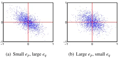
Fig. 2. Toy data. The value ofkYk2
Ffor left (right) is 264.4 (261.8). On the
other hand, the overall quantization error for left (right) is 2642.5 (2628.3).
wherek · kF denotes the Frobenius norm of matrix. Based on
the constraints, it is easy to verify that the projection error (re-construction error mentioned above) can be computed as
ep=kX−YPTk2F =kXk2F− kXPk2F (2)
SincekXk2
Fis a constant, by substituting Equation (2) into
prob-lem (1), we obtain the final objective function of PCA, max
P kXPk 2
F, s.t.PTP=Ik (3)
which can be regard as maximizing the total variance of pro-jected data because the data is zero centered. Problem (3) can be efficiently optimized by eigenvalue decomposition.
The projectionPobtained above can preserve the global Eu-clidean structure, i.e., it satisfies the first property. Now let us consider the second property, minimizing quantization er-ror. Given real-value data Y, and corresponding binary codes
B =sign(Y), the quantization error caused by sign function is
defined as the distance between them as follows,
eq=kB−Yk2F =kBk2F+kYk2F−2kYk1 (4)
wherekYk1 = Pi,j|yi j|. We have the last term above because
bi j = sign(yi j) ⇒ bi jyi j = |yi j|. Since we havekBk2F = nkis
a constant andY=XP, the projection which can minimize the
quantization error can be learned as below max
P 2kXPk1− kXPk 2
F, s.t.PTP=Ik (5)
Comparing problem (3) to (5), we can obtain an interesting observation: directly maximizing (5) longs for smallerkXPk2
F
which is against maximizing (3). In most situations, the respec-tive optimal solutions to (3) and (5) are different.
Above we show the direct connection and contradiction between minimizing projection error and quantization error. However, such relationship between above two errors is ignored in previous works (Gong and Lazebnik, 2011; Kong and Li, 2012b). Consequently, a greedy two-step strategy considering two properties separatelyis widely adopted. One representa-tive work is Iterarepresenta-tive Quantization (ITQ) (Gong and Lazebnik, 2011). Specifically, they first optimize problem (3) and obtain an initial projection P. Then a rotation matrix R ∈ Rk×k is
learned by a Procrustean approach to minimize the quantiza-tion error from projected dataY=XP. The objective function
of ITQ can be formulated as follows, min
B,R kB−YRk 2
[image:5.595.59.258.62.164.2]F, s.t., B=sign(YR),RRT =Ik (6)
Table 1.epandeq(×104) on SIFT1M.
ep eq
ITQ OPH ∆OPH ITQ OPH ∆OPH
16 bits 17.69 17.95 +1.47% 13.97 12.74 −8.80%
32 bits 10.29 10.56 +2.62% 14.31 12.51 −12.58%
64 bits 3.82 3.92 +2.61% 19.22 16.78 −12.70%
96 bits 1.17 1.20 +2.56% 28.07 25.11 −10.47%
The final projection is given byPR. A rotation matrix satisfies
tr(RTYR) =tr(Y) for any square matrix. SoPRmust be the
optimal solution to problem (3) too. Hence, their basic idea can be summarized as: first minimizing projection error, then min-imizing quantization errorwhile fixing projection error. Since kXPk2
Fis fixed now, problem (5) in a two-step strategy could be
rewritten as formulation below
max
P kXPk1, s.t.P
TP=I
k,kXPk2F =c (7)
wherecis the optimal value of problem (3). Here, the extra con-straint limits the feasible set ofPhence the obtained projection may be onlysub-optimalfor the second property.
Let us take the toy data in Figure 2 as an example. Suppose we have two different orthogonal projectionsP1andP2for
orig-inal dataXand map data to 2-dimensional space, and then we solve problem (6) to find the rotation which can minimize the quantization error given the initial projection, whose results are shown in 2(a) and 2(b) respectively. The value of kXP1k2F is
larger than kXP2k2F, indicating that P1 is a better solution to
problem (3) and has smaller projection error based on Equation (2). However, after an optimal rotation, the quantization error in 2(a) islargerthan in 2(b), implying that the extra constraint fromkXP1k2F = cindeed leads to a worse optimal solution to
problem (7). In addition, intuitively we also prefer the result in 2(b). Consequently we can say 2(b) achieves a betteroverall performancefor both properties than 2(a), even if its projection is indeed not the optimum for the first property.
ACCEPTED MANUSCRIPT
quantization error while increase little projection error, i.e., wecan find a better trade-offbetween them such that the overall
error is minimized; and 2) the two-step strategy indeed leads tosub-optimalsolution because the results from initial projec-tion limit the feasible soluprojec-tion set for problem (7). Considering the ultimate goal is to generate binary Hashcodes from original features, the projection learning should take into account both preserving information and minimization quantization error si-multaneously, but not separately as ITQ. Therefore it is more reasonable to learn an optimal projection function via jointly optimizingthe projection and quantization error.
3. Learning Optimized Projection
3.1. Objective Function
The observation in Section 2 is based on PCA projection. However, the phenomenon can be observed for other projec-tions, such as in Spectral Hashing (Weiss et al., 2008). To make our formulation general, i.e., it can be incorporated into diff
er-ent projections, we first need to investigate the projection and quantization error for different projections. Observed from
lit-eratures (Jegou et al., 2010; Kumar and Udupa, 2011; Liu et al., 2011; Weiss et al., 2008; Zhang et al., 2011), the following pro-jection learning formulation is widely adopted,
max
P tr(P
TXTWXP), s.t.PTP=I
k (8)
whereW∈Rn×nis a weight matrix. Actually, according to the
specific situations, we need to preserve different information in
original data hence differentWcan be adopted. For example,
when global Euclidean structure is concerned about (Gong and Lazebnik, 2011; Jegou et al., 2010; Kong and Li, 2012b), like in PCA, we setW=Ikand problem (8) is identical to problem
(3); when we want to exploit the local manifold structure, i.e., we want to preserve the local neighborhood relationship be-tween data, like Spectral Hashing (Weiss et al., 2008), Anchor Graph Hashing (Liu et al., 2011) and Locality Preserving Hash-ing (Zhao et al., 2014), we can adopt thenormalizedadjacency matrix constructed from nearest neighbor graph; to preserve the pair-wise label information, such as in Semi-supervised Hash-ing(Wang et al., 2010), we can adopt the label-sharing matri.
With the formulation in (8), the projection error is no longer just the reconstruction error in Euclidean space. But we can define the projection error analogous to PCA below,
Definition 1. Given a weight matrixW, the projection error is defined as the loss of weighted similarity among data,
ep= n
X
i=1
n
X
j=1
wi jxixTj − n
X
i=1
n
X
j=1
wi j(xiP)(xjP)T
=tr(XTWX)−tr(PTXTWPX), PTP=Ik
(9)
It is not difficult to verify that theep defined in Equation (2) is
a special case of (9) withW=In. Also, since the first term is
fixed, minimizing projection error in above definition is equiv-alent to problem (8). Furthermore, here is another explanation for above definition. The essential purpose of Hashing is to
preserve data similarity, i.e., the similar points should be sim-ilar after projection. Therefore, given a simsim-ilarity measure (in this paper, we adopt the weighted inner product as (Wang et al., 2010)), the overall loss of data similarity resulted from a pro-jection reflects how well it preserves the similarity.
The generalized projection error in DEFINITION 1 consid-ers the information preserving property, and the quantization er-ror in Equation (4) considers the other property. Intuitively, we can jointly optimize them such that the overall result is better, as illustrated in Table 1. Specifically, we can define the overall error under a projection Pas the weighted sum of projection and quantization error as follows
e=λep+eq=c+tr(PTXT(In−λW)XP)−2kXPk1 (10)
wherec=tr(XTWX)+nkis a constant, andλis the weight pa-rameter. Therefore we just need to minimize such overall error to learn optimized projection. Based on the unified formulation, we can obtain the objective function forOptimized Projection
in a general learning framework as
max
P O=tr(P
TXTAPX)+kXPk
1, s.t.PTP=Ik (11)
whereA= 12(λW−In). As we have mentioned, we formulate
this framework to be general such that it can be incorporated with different Hashing methods given specificW. SettingW=
In, we obtain the learning problem below
max
P OPCA=αkXPk 2
F+kXPk1, s.t.PTP=Ik (12)
whereα= 12(λ−1). Above is the joint optimization framework of PCA, which optimizes the overall performance of preserv-ing global Euclidean structure and minimizpreserv-ing quantization er-ror, which is intrinsically different from ITQ which optimizes
them separately. Our results shown in Table 1 are obtained by it. We can see we do not aim at optimizing either of it, but focus on finding a good trade-off which, compared to ITQ, works slightly worse for projection but much better for quan-tization. Such formulation looks simple but not trivial. To our best knowledge, we are the first tonotice and analyzethe con-nection between the projection error and quantization error, and
empirically provethe reasonability and effectiveness of (12).
Another important information in data is the local manifold structure (Cai et al., 2011). In CBDR task, we care more about obtaining data sharing the same semantic label as the query where manifold distance is a better measure than global Eu-clidean distance (Liu et al., 2011). Preserving the manifold structure is always formulated as preserving the local nearest neighbor (NN) relationship in data. Specifically, we can con-struct ap-NN graph with the weight of each edge as below
Si j =
e−
kxi−xjk2
σ , ifxi∈ N(xj) orxj∈ N(xi)
0, otherwise (13)
whereN(xi) is the p-NN ofxiandσis the band width (Guo
et al., 2017b). Then we obtain a diagonal degree matrix D
whose diagonal elements areDii =Pnj=1Si j. Now we can
de-fineWas thenormalizedadjacency matrix for thep-NN graph
ACCEPTED MANUSCRIPT
With this symmetric normalized adjacency matrix, we can learnan optimized projection by (11) which can find a good trade-offbetween preserving local manifold structure and minimizing
quantization error. We can also utilize other definitions ofW
for specific purposes. But because of the limitation of space, in this paper we just incorporate OPH with two of the most widely used deifnitions. These two simple definitions can yet lead to state-of-the-art performance.
3.2. Learning Algorithm
Considering problem (12) is just a special case of problem (11), we only show the learning algorithm for (11). In this pa-per, we use the gradient flow (Wen and Yin, 2013) to solve the orthogonality constrained `1 norm regularized
maximiza-tion problem. Obviously, we can also utilize some accelerated proximal gradient methods (APG) for optimization (Lan et al., 2015, 2018). But to make the algorithm more general, we still use the original one. The basic idea is to firstly find the upgra-dient at a point, secondly project the upgraupgra-dient to the tangent space of feasible set defined by the orthogonality constraint, and thirdly move the point with a properly small step size to-wards this direction in the feasible set. We can iterate above three steps until convergence. Specifically, the feasible set for the solution is defined asMP ={P∈Rd×k:PTP=Ik}. Given
pointPt∈ MP, we first compute theupgradientofOatPt
Ut=−DO(Pt)=−XT(AXPt+sign(XPt)) (15)
To projectUtto tangent space, we need the theorem below,
Theorem 1. Given a directionUt atPt, the projection of Ut
onto the tangent space ofMPatPtis computed below
Dt=MtPt, whereMt=UtPTt −PtUTt (16)
The detailed proof can be found in (Wen and Yin, 2013). Then we need to movePtto a new pointPt+1. Directly moving it like
in conventional gradient descent (Pt+1 = Pt−τDt) will move
Pt+1out of the feasible set. So in practice (Goldfarb et al., 2009;
Vese and Osher, 2002; Wen and Yin, 2013), we will compute the next point by the Crank-Nicolson-like scheme:
Pt+1=Pt−τMt(Pt+2Pt+1) (17)
which can lead to the following closed form solution forPt+1
Pt+1 =(Id+τ2Mt)−1(Id−τ2Mt)Pt (18)
Above updating rule is called Cayley transformation and τis a step size satysfying Armijo-Wolfe conditions (Nocedal and Wright, 1999). Considering thatUt is a skew-symmetric
ma-trix, i.e.,UT
t =−Ut, the matrixId+τ2Mtis definitely invertable
andPt+1 is also orthogonal, i.e., Pt+1 ∈ MP, and it results in
nonincreasing objective function value. For more detail please see the proof to Lemma 3 in (Wen and Yin, 2013). We can ran-domly generate an orthogonal matrix to initializePand repeat above steps until a stationary point is achieved, i.e.,Pt+1 =Pt,
which is the solution to problem (11). The overall learning al-gorihm for Optimized Projection is summarized in Algorithm 1. To this end, the Hashing function is given ash(x)=sign(xP).
Algorithm 1Learning Optimized Projection
Input:
Training matrixX, Hashcode lengthk, weight matrixW, balance parameterλ Output:
Optimized ProjectionP
1: ConstructA= 12(λW−In);
2: InitializeP0by a random orthogonal matrix, t=0
3: repeat
4: Compute the upgradientUtby (15);
5: Compute the skew-symmetric matrixMtby (16); 6: Compute the new pointPt+1by (18);
7: t=t+1;
8: untilConvergence.
9: ReturnPt;
4. Discussion
Now we discuss the time complexity of Algorithm 1. The time complextity to compute the upgradientUtisO(ndk+n2k),
to compute the skew-symmetric matrix isO(d2k). And to
com-pute new point by Equation (18), the complexity is O(d2k+ dk2 +k3). Actually, the complextity for inverting an
arbi-trary d ×d matrix should be O(d3). However, since we
al-ways havek d, especially for high-dimensional image and text data, the rank of matrixMt is at most 2k. Hence
follow-ing the Sherman-Morrison-Woodbury theorem (Sherman and Morrison, 1950), the complexity for inverting (Id + τ2Mt) is
O(dk2+k3). Therefore, the overall complextity for Algorithm 1
isO(t(ndk+n2k+d2k+dk2+k3)), wheretis the number of
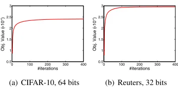
itera-tions to convergence. In Figure 3, we plot the objective function value w.r.t. the number of iterations on two real-world datasets under different Hashcode length. Here we setW=In, i.e., we
incorporate OPH with PCA. We can observe that the objective function value increases steadily with more iterations, and it can converge within 200 iterations, validating the effectiveness
of Algorithm 1, which also guarantees the training efficiency.
In above section, we have mentioned that the proposed OPH can be incorporated with different Hashing methods who have
ACCEPTED MANUSCRIPT
0 100 200 300 400 0.5
1 1.5 2 2.5 3
#iterations
Obj. Value (
×
10
5)
(a) CIFAR-10, 64 bits
0 100 200 300 400 0.5
1 1.5 2 2.5 3
#iterations
Obj. Value (
×
10
5)
[image:8.595.66.246.60.151.2](b) Reuters, 32 bits
Fig. 3. Objective function w.r.t.#iterations.
et al., 2013) which is derived from Spectral Hashing. It finds a rotation to minimize the distance between the rotated data and a matrix whose variance of each dimension is close. How-ever, such strict requirement and its non-iterative optimization algorithm may fail to find a good enough solution. Above three methods all adopt two-step strategy so their overall per-formance is worse than OPH. Furthermore, those three meth-ods are derived from specific projection and there is no clue that they can still perform satisfactorily when combined with other projections. But OPH is quite general and based on the generalized projection error defined in Equation (9). It is ro-bust to different projections, which will be demonstrated in our
experiments.
5. Experiment
5.1. Baselines, Metrics and Settings
We utilize the following related Hashing methods. Lo-cality Sensitive Hashing (LSH) (Andoni and Indyk, 2006), PCA Hashing (PCAH) (Jegou et al., 2010), Spectral Hashing (SpH) (Weiss et al., 2008), Anchor Graph Hashing (AGH) (Liu et al., 2011) with two-layer Hashing function, Iterative Quan-tization (ITQ) (Gong and Lazebnik, 2011), Isotropic Hash-ing (IsoH) (Kong and Li, 2012b), and Harmonious HashHash-ing (HamH) (Xu et al., 2013). For meaningful comparison, we carefully tuned the model parameters for all baselines and the best performance is shown.
Recently, some deep learning based hashing approaches (Lai et al., 2015; Liong et al., 2015; Liu et al., 2016; Xia et al., 2014; Zhuang et al., 2016) have achieved promising results. However, it should be noted that they mostly focus on image hashing and using raw pixels as input, while our approaches and selected baselines focus on feature hashing which is more flexible so that they can use any kinds of features as input. Therefore, we do not choose deep hashing approaches as baselines.
We adopt mean Average Precision (mAP) as the numeric evaluation metric. mAP shows good discriminative power and stability to evaluate the performance of retrieval task. A larger mAP indicates better performance that true positive samples have higher rank. Given a query andRretrieved samples based on Hamming ranking, the Average Precision (AP) is
AP= 1
L
R
X
r=1
P(r)δ(r) (19)
whereLis the number of true positive samples in the retrieved set,P(r) denotes the precision of toprretrieved samples defined as the ratio between the number true positive samples and the number of retrieved samples (i.e., r), and δ(r) is an indicator function which is equal to 1 if ther-th sample is true positive or 0 otherwise. Averaging the AP of all queries leads to mAP. We also adopt the Precision-Recall curve and the Recall curve.
In this paper, we implement two Hashing methods based on OPH. The first utilizes PCA projection, i.e., the projection is learned by problem (12). When implementing it, the parameter
αis chosen from{0.01,0.1,1}based on the change in projection and quantization error in training data compared to ITQ. We select the value which maximizes the sum of∆OPHforepandeq.
This method is denoted as PCA-OPH. The second considers the local manifold structure, i.e., the weight matrixWis defined as in Equation (14) and constructed from ap-NN graph where we setpas 0.1% of training data. The parameterλis chosen from {0.1,1,2,5,10}. This method is denoted as Sp-OPH following
Spectral Hashing. When learningPwith Algorithm 1, we stop at the 200th itertation. The binary Hashcodes of a new coming sample x is computed by h(x) = sign((x−x¯)P), where ¯x is
the mean value of training data which is utilized to centralize training data. For fair comparison, our baseline methods also adopt such schema for generating Hashcodes.
When compute mAP, we setR=50. To remove any
random-ness caused by random initialization or random training data selection, all results are the average over 10 repeated runs. All experiments are carried out on a computer which equips Intel Core i7-2600 CPU @3.40GHz and 16GB RAM.
5.2. Approximate Nearest Neighbor Search 5.2.1. Datasets
The ANN search is a practical and important task in real world. Its purpose is to find some Euclidean neighborhood from database for a given query. In this task, we adopt two widely used large-scale and high-dimensional datasets. The first dataset is SIFT1M (Jegou et al., 2011) which consists of 1 mil-lion 128-dimension SIFT (Lowe, 2004) points and 10,000 inde-pendent points as the query. The second is GIST1M (Torralba et al., 2008) containing 1 million 960-dimension GIST (Oliva and Torralba, 2001) poits and 1,000 independent queries. Fol-lowing (Gong and Lazebnik, 2011; Kong and Li, 2012b; Xu et al., 2013), for each query, its true positive samples are the first 100 nearest neighbors in database obtained by brute force search with Euclidean distance. And to test the ability of diff
er-ent Hashing methods to deal with out-of-sample data, we ran-domly select 10,000 points from database as the training data to learn Hashing functions. Then we generate Hashcodes for samples in both database and query set by the learned Hashing functions as in (Ding et al., 2014; Song et al., 2013).
5.2.2. Results
ACCEPTED MANUSCRIPT
0 5000 10000
0 0.2 0.4 0.6 0.8 1
N(# of top Hamming neighbors)
Recall
(a) SIFT1M, 16 bits
0 5000 10000
0 0.2 0.4 0.6 0.8 1
N(# of top Hamming neighbors)
Recall
(b) SIFT1M, 32 bits
0 5000 10000
0 0.2 0.4 0.6 0.8 1
N(# of top Hamming neighbors)
Recall
(c) SIFT1M, 64 bits
0 5000 10000
0 0.2 0.4 0.6 0.8 1
N(# of top Hamming neighbors)
Recall
LSH PCAH SpH AGH ITQ HamH IsoH PCA−OPH Sp−OPH
[image:9.595.77.506.65.165.2](d) SIFT1M, 96 bits
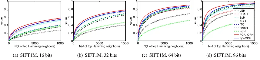
Fig. 4. ANN search. Recall curves on SIFT1M with different Hashcode length.
0 5000 10000
0 0.2 0.4 0.6
N(# of top Hamming neighbors)
Recall
(a) GIST1M, 16 bits
0 5000 10000
0 0.2 0.4 0.6
N(# of top Hamming neighbors)
Recall
(b) GIST1M, 32 bits
0 5000 10000
0 0.2 0.4 0.6
N(# of top Hamming neighbors)
Recall
(c) GIST1M, 64 bits
0 5000 10000
0 0.2 0.4 0.6
N(# of top Hamming neighbors)
Recall
LSH PCAH SpH AGH ITQ HamH IsoH PCA−OPH Sp−OPH
(d) GIST1M, 96 bits
Fig. 5. ANN search. Recall curves on GIST1M with different Hashcode length.
More extensive results are given in Figures 4 and 5. We can observe that PCA-OPH achieve best performance in all experi-ments and markedly outperform the two-step methods (ITQ and IsoH) in most cases. And Sp-OPH also outperforms baselines in most experiments and it shows superior performance to the two-step HamH in 10 out of 12 experiments. Such results val-idate the effectiveness of OPH for ANN search. Moreover, we
can observe the following points.
Firstly, OPH achieves more improvement over ITQ, IsoH and HamH with shorter Hashcodes. Besides, the improvement is more obvious on GIST1M (960 dimensions) than SIFT1M (128 dimensions). The reason is as below. For shorter Hashcodes, OPH needs to pick fewer directions such that it has more free-dom hence it can find a better trade-off from a large number
of candidates. However, for two-step methods, its feasible set is limited by the initial projection. Actually, fewer directions lead to more limitation therefore the overall solution is farther from the optimum. In addition, we can even observe that ITQ performs worse than PCAH in some cases, typically with short Hashcodes. This phenomenon also demonstrates that the initial projection will limit the following adjustment step and the two-step strategy leads to sub-optimal solution. With longer Hash-codes, ITQ has more freedom after initial projection so we can observe it significantly outperforms PCAH. But it still suffers
from some limitation to some extent such that its overall result is worse than OPH. This result validates again the reasonability of the unified formulation adopted in OPH.
Secondly, OPH and methods considering the quantization error, such as ITQ, perform much better with longer Hash-codes, while methods like PCA may perform worse. Such in-teresting phenomenon has also been observed by previous re-searchers (Gong and Lazebnik, 2011; Wang et al., 2010; Xu
et al., 2013). Intuitively, longer Hashcodes can encode more information thus better results are expected. However, the vari-ance in PCA projected data is quite imbalvari-anced and many di-mensions in long Hashcodes contain little information such that they may severely degrade the overall quality of long Hash-codes. Because of the quantization step, the information pre-served in the projection may be destroyed. So considering the quantization error is important for projection learning.
5.3. Content-based Image Retrieval
5.3.1. Datasets
Hashing has been widely utilized in Content-based Image Retrieval (CBIR) (Ding et al., 2014; Gong and Lazebnik, 2011; Guo et al., 2015; Liu et al., 2011; Zhou et al., 2014). Different
ACCEPTED MANUSCRIPT
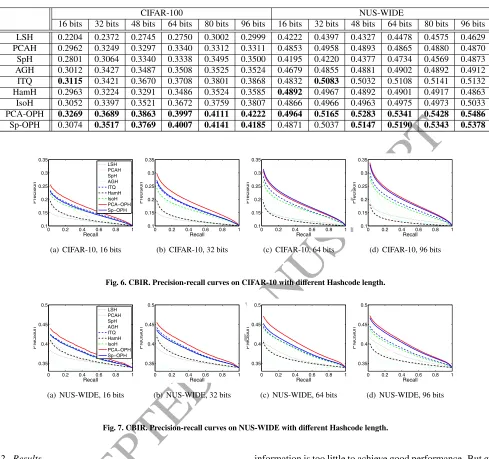
Table 2. mAP Comparison. The bold numbers indicate the best two results.CIFAR-100 NUS-WIDE
16 bits 32 bits 48 bits 64 bits 80 bits 96 bits 16 bits 32 bits 48 bits 64 bits 80 bits 96 bits
LSH 0.2204 0.2372 0.2745 0.2750 0.3002 0.2999 0.4222 0.4397 0.4327 0.4478 0.4575 0.4629
PCAH 0.2962 0.3249 0.3297 0.3340 0.3312 0.3311 0.4853 0.4958 0.4893 0.4865 0.4880 0.4870
SpH 0.2801 0.3064 0.3340 0.3338 0.3495 0.3500 0.4195 0.4220 0.4377 0.4734 0.4569 0.4873
AGH 0.3012 0.3427 0.3487 0.3508 0.3525 0.3524 0.4679 0.4855 0.4881 0.4902 0.4892 0.4912
ITQ 0.3115 0.3421 0.3670 0.3708 0.3801 0.3868 0.4832 0.5083 0.5032 0.5108 0.5141 0.5132
HamH 0.2963 0.3224 0.3291 0.3486 0.3524 0.3585 0.4892 0.4967 0.4892 0.4901 0.4917 0.4863
IsoH 0.3052 0.3397 0.3521 0.3672 0.3759 0.3807 0.4866 0.4966 0.4963 0.4975 0.4973 0.5033
PCA-OPH 0.3269 0.3689 0.3863 0.3997 0.4111 0.4222 0.4964 0.5165 0.5283 0.5341 0.5428 0.5486
Sp-OPH 0.3074 0.3517 0.3769 0.4007 0.4141 0.4185 0.4871 0.5037 0.5147 0.5190 0.5343 0.5378
0 0.2 0.4 0.6 0.8 1 0.1
0.15 0.2 0.25 0.3 0.35
Recall
Precision
LSH PCAH SpH AGH ITQ HamH IsoH PCA−OPH Sp−OPH
(a) CIFAR-10, 16 bits
0 0.2 0.4 0.6 0.8 1 0.1
0.15 0.2 0.25 0.3 0.35
Recall
Precision
(b) CIFAR-10, 32 bits
0 0.2 0.4 0.6 0.8 1 0.1
0.15 0.2 0.25 0.3 0.35
Recall
Precision
(c) CIFAR-10, 64 bits
0 0.2 0.4 0.6 0.8 1 0.1
0.15 0.2 0.25 0.3 0.35
Recall
Precision
(d) CIFAR-10, 96 bits
Fig. 6. CBIR. Precision-recall curves on CIFAR-10 with different Hashcode length.
0 0.2 0.4 0.6 0.8 1 0.35
0.4 0.45 0.5
Recall
Precision
LSH PCAH SpH AGH ITQ HamH IsoH PCA−OPH Sp−OPH
(a) NUS-WIDE, 16 bits
0 0.2 0.4 0.6 0.8 1 0.35
0.4 0.45 0.5
Recall
Precision
(b) NUS-WIDE, 32 bits
0 0.2 0.4 0.6 0.8 1 0.35
0.4 0.45 0.5
Recall
Precision
(c) NUS-WIDE, 64 bits
0 0.2 0.4 0.6 0.8 1 0.35
0.4 0.45 0.5
Recall
Precision
(d) NUS-WIDE, 96 bits
Fig. 7. CBIR. Precision-recall curves on NUS-WIDE with different Hashcode length.
5.3.2. Results
The mAP comparison on two datasets among different
meth-ods with various Hashcode length is summarized in Table 2, and the corresponding Precision-recall curves are shown in Fig-ures 6 and 7. We can observe OPH outperforms other baseline methods regardless of the datasets and Hashcode length, which demonstrates the superiority of OPH for CBIR task. And we have other two important observations.
Firstly, our OPH improves the performance over ITQ and other baselines more with longer Hashcodes. This observation is different from the one in ANN task but in fact they are not
contradictory at all. In ANN, the data distribution is simple and we care about the Euclidean neighbors. As we have dis-cussed above, the freedom to select directions is important for ANN. In contrast, CBIR faces more complicated data distri-bution and we care about high-level semantic relationship be-tween data. In such situation, encoding information effectively
becomes the key problem. With short Hashcodes, the available
information is too little to achieve good performance. But given long Hashcodes, more information is available. Our OPH can preserve more information from original data to Hashcodes be-cause it adopts a unified framework considering the overall per-formance while the two-step strategy in ITQ, IsoH and HamH can only obtains sub-optimal solution. In addition, the itera-tive optimization strategy in ITQ and IsoH leads to local opti-mum. With longer Hashcodes and more variables, their local optimum will be farther from the global optimum therefore the performance gap between OPH and them will be larger.
ACCEPTED MANUSCRIPT
Table 3. mAP Comparison. The bold numbers indicate the best two results.TDT2 Reuters
16 bits 32 bits 48 bits 64 bits 80 bits 96 bits 16 bits 32 bits 48 bits 64 bits 80 bits 96 bits
LSH 0.4270 0.6368 0.7447 0.7750 0.8246 0.8515 0.5918 0.6439 0.6902 0.7298 0.7448 0.7717
PCAH 0.6488 0.7348 0.7455 0.7672 0.8047 0.8105 0.6844 0.7203 0.7579 0.7978 0.7964 0.7990
SpH 0.3291 0.3678 0.4103 0.4726 0.4783 0.5082 0.4977 0.6162 0.6415 0.6592 0.6641 0.6739
AGH 0.4183 0.6181 0.7416 0.7488 0.7659 0.7683 0.4513 0.5821 0.6569 0.7150 0.7282 0.7297
ITQ 0.6629 0.7529 0.7902 0.8368 0.8286 0.8638 0.6977 0.7724 0.7916 0.8012 0.8061 0.8172
HamH 0.6788 0.7548 0.7855 0.7972 0.8147 0.8205 0.7344 0.7703 0.7879 0.7978 0.7964 0.7990
IsoH 0.7032 0.7683 0.8131 0.8349 0.8523 0.8604 0.6826 0.7518 0.7739 0.7849 0.7992 0.8042
PCA-OPH 0.7288 0.7740 0.8428 0.8727 0.8978 0.9094 0.7357 0.7830 0.8162 0.8376 0.8489 0.8507
Sp-OPH 0.6807 0.7641 0.8205 0.8495 0.8602 0.8785 0.6537 0.7682 0.7859 0.8144 0.8231 0.8375
0 0.2 0.4 0.6 0.8 1 0
0.2 0.4 0.6 0.8 1
Recall
Precision
LSH PCAH SpH AGH ITQ HamH IsoH PCA−OPH Sp−OPH
(a) TDT2, 16 bits
0 0.2 0.4 0.6 0.8 1 0
0.2 0.4 0.6 0.8 1
Recall
Precision
(b) TDT2, 32 bits
0 0.2 0.4 0.6 0.8 1 0
0.2 0.4 0.6 0.8 1
Recall
Precision
(c) TDT2, 64 bits
0 0.2 0.4 0.6 0.8 1 0
0.2 0.4 0.6 0.8 1
Recall
Precision
(d) TDT2, 96 bits
Fig. 8. CBTR. Precision-recall curves on TDT2 with different Hashcode length.
0 0.2 0.4 0.6 0.8 1 0.3
0.4 0.5 0.6 0.7 0.8
Recall
Precision
LSH PCAH SpH AGH ITQ HamH IsoH PCA−OPH Sp−OPH
(a) Reuters, 16 bits
0 0.2 0.4 0.6 0.8 1 0.3
0.4 0.5 0.6 0.7 0.8
Recall
Precision
(b) Reuters, 32 bits
0 0.2 0.4 0.6 0.8 1 0.3
0.4 0.5 0.6 0.7 0.8
Recall
Precision
(c) Reuters, 64 bits
0 0.2 0.4 0.6 0.8 1 0.3
0.4 0.5 0.6 0.7 0.8
Recall
Precision
(d) Reuters, 96 bits
Fig. 9. CBTR. Precision-recall curves on Reuters with different Hashcode length.
after initial projection. This result implies that the optimization algorithm of HamH is less effective than ITQ and IsoH in
prac-tice. We need to say that the adjustment in HamH helps to some extent because HamH is still better than SpH and AGH. This re-sult also reveals the importance of optimization. The superior results of Sp-OPH over ITQ and IsoH show our unified learning framework indeed works.
5.4. Content-based Text Retrieval 5.4.1. Datasets
The Content-based Text Retrieval (CBTR) is analogous to CBIR except it is for text data which is another application of Hashing (Salakhutdinov and Hinton, 2009). In this task, two benchmark datasets are involved. The first is TDT2 (J-Fiscus et al., 1999) collected from newswires, radio and tele-vision programs. It contains 64,527 documents classified into 100 semantic categories. Each document is represented by a term frequency-inverted document frequency (tf-idf) vector
with 36,771 dimensions. The other is Reuters (Lewis et al., 2004) dataset which consists of 21,578 documents from 135 categories. For each document, we use a 18,933-dimension tf-idf vector as original feature. For both datasets, we randomly select 1,000 documents as the query set and the remained form the database. We construct the training set by randomly select-ing 10,000 documents from database. True positives are docu-ments sharing labels with the query.
5.4.2. Results
ACCEPTED MANUSCRIPT
16 32 48 64 80 96 0.3
0.34 0.38 0.42 0.46
#bits
mAP
α=0.01
α=0.1 α=1
(a) CIFAR-10
16 32 48 64 80 96 0.7
0.76 0.82 0.88 0.94
#bits
mAP
α=0.01
α=0.1 α=1
(b) TDT2
16 32 48 64 80 96 0.7
0.74 0.78 0.82 0.86
#bits
mAP
α=0.01
α=0.1 α=1
[image:12.595.134.488.67.403.2](c) Reuters
Fig. 10. mAP of PCA-OPH w.r.t.α.
5 10 20 30 40 50 0.38
0.39 0.4 0.41 0.42
training size ×103
mAP
PCA−OPH Sp−OPH
(a) CIFAR-10, 64 bits
5 10 20 30 40 50 0.52
0.53 0.54 0.55 0.56
training size ×103
mAP
PCA−OPH Sp−OPH
(b) NUS-WIDE, 96 bits
5 10 20 30 40 50 0.87
0.88 0.89 0.9 0.91 0.92
training size ×103
mAP
PCA−OPH Sp−OPH
(c) TDT2, 96 bits
Fig. 11. mAP of OPH w.r.t. training size.
However, Sp-OPH is consistently worse than PCA-OPH in all experiments for CBTR. One possible reason might be that the
p-NN graph is less precise in high-dimensional data like text given the imprecise distance computing, and the local manifold structure can not be effectively exploited with such low-quality
graph. But in PCA-OPH, we do not need to compute the dis-tancebetweendata thus such problem can be avoided.
5.5. Other Issues
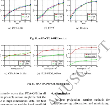
Now we investigate the balance parameter in OPH. For sim-plicity, we show the effect of α on PCA-OPH. This param-eter controls the balance of projection error and quantization error. Results on CIFAR-10, TDT2 and Reuters with diff
er-ent αare plotted in Figure 10. Indeed, the value ofαhas in-fluence on OPH to some extent, but we can also notice that statisfactory trade-offcan be obtained with a properα. Typi-cally,α∈[0.01,1] always works. Actually, ifαis too big (like 10,000), PCA-OPH degenerates to PCAH.
Then we show the effect of the size of training data. The
performance of PCA-OPH and Sp-OPH on CIFAR-10, NUS-WIDE and TDT2 is plotted in Figure 11. Given more training data, OPH can perform slightly better because more informa-tion is available. But it is also obvious that the improvement is quite small when the size is larger than 10,000. When the training size grows from 10,000 to 50,000, the improvement in mAP is less than 0.01. In fact, given enough training data (say, 10,000), the model can be well trained and extra data is redun-dant. This phenomenon is also observed in baseline methods, like PCAH, ITQ, AGH, and etc.
6. Conclusion
Previous projection learning methods for Hashing con-sider preserving information and minimizing quantization er-ror seperately. In this paper, we empirically study this prob-lem and prove that only sub-optimal solution can be achieved in this two-step strategy. Hence we propose a unified and gen-eral projection learning framework for Hashing to find the best trade-offbetween them and learn an Optimized Projection for
better overall performance. An effective optimization algorithm
is given. Extensive experiments for ANN and CBDR on several benchmarks compared to state-of-the-art related Hashing meth-ods validate the effectiveness of OPH.
Acknowledgments
This research was supported by the National Natural Science Foundation of China Grant No. 61571269, and the Royal Soci-ety Newton Mobility Grant IE150997.
References
Andoni, A., Indyk, P., 2006. Near-optimal hashing algorithms for approximate nearest neighbor in high dimensions, in: FOCS’06, pp. 459–468.
Cai, D., He, X., Han, J., Huang, T.S., 2011. Graph regularized nonnegative matrix factorization for data representation. IEEE TPAMI 33, 1548–1560. Chen, L., Xu, D., Tsang, I.W., Li, X., 2014. Spectral embedded hashing for
scalable image retrieval. IEEE T. Cybernetics 44, 1180–1190.
Chua, T., Tang, J., Hong, R., Li, H., Luo, Z., Zheng, Y., 2009. NUS-WIDE: a real-world web image database from national university of singapore, in: CIVR.
Ding, G., Guo, Y., Zhou, J., 2014. Collective matrix factorization hashing for multimodal data, in: CVPR, pp. 2083–2090.
ACCEPTED MANUSCRIPT
(a) 32 bits (b) 64 bits (c) 96 bits
Fig. 12. Top 5 retrieved images for query (left) by LSH (up), PCAH, AGH, ITQ, and PCA-OPH (down).
Friedman, J.H., Bentley, J.L., Finkel, R.A., 1977. An algorithm for finding best matches in logarithmic expected time, in: ACM Trans. Mathematical Software, pp. 209–226.
Gionis, A., Indyk, P., Motwani, R., 1999. Similarity search in high dimensions via hashing, in: VLDB, pp. 518–529.
Goldfarb, D., Wen, Z., Yin, W., 2009. A curvilinear search method for the p-harmonic flow on spheres. SIAM J. Imaging Sci 2, 84–109.
Gong, Y., Lazebnik, S., 2011. Iterative quantization: A procrustean approach to learning binary codes, in: CVPR, pp. 817–824.
Guo, Y., Ding, G., Han, J., 2018. Robust quantization for general similarity search. IEEE Trans. Image Processing 27, 949–963.
Guo, Y., Ding, G., Han, J., Gao, Y., 2017a. Sitnet: Discrete similarity transfer network for zero-shot hashing, in: IJCAI, pp. 1767–1773.
Guo, Y., Ding, G., Han, J., Gao, Y., 2017b. Zero-shot learning with transferred samples. IEEE Trans. Image Processing 26, 3277–3290.
Guo, Y., Ding, G., Jin, X., Wang, J., 2015. Learning predictable and discrimi-native attributes for visual recognition, in: AAAI, pp. 3783–3789. Guo, Y., Ding, G., Liu, L., Han, J., Shao, L., 2017c. Learning to hash with
optimized anchor embedding for scalable retrieval. IEEE Trans. Image Pro-cessing 26, 1344–1354.
He, K., Wen, F., Sun, J., 2013. K-means hashing: an affinity-preserving
quan-tization method for learning binary compact codes, in: CVPR, pp. 2938– 2945.
J-Fiscus, Doddington, G.R., Garofolo, J.S., Martin, A.F., 1999. Nist’s 1998 topic detection and tracking evaluation (TDT2), in: EUROSPEECH. Jegou, H., Douze, M., and, C.S., 2011. Product quantization for nearest
neigh-bor search. TPAMI 33, 117–128.
Jegou, H., Douze, M., Schmid, C., P´erez, P., 2010. Aggregating local descrip-tors into a compact image representation, in: CVPR, pp. 3304–3311. Kong, W., Li, W.J., 2012a. Double-bit quantization for hashing., in: AAAI. Kong, W., Li, W.J., 2012b. Isotropic hashing, in: NIPS, pp. 1655–1663. Krizhevsky, A., 2009. Learning multiple layers of features from tiny images.
Tech Report. Univ. of Toronto .
Kumar, S., Udupa, R., 2011. Learning hash functions for cross-view similarity search, in: IJCAI, pp. 1360–1365.
Lai, H., Pan, Y., Liu, Y., Yan, S., 2015. Simultaneous feature learning and hash coding with deep neural networks, in: CVPR, pp. 3270–3278.
Lan, X., Ma, A.J., Yuen, P.C., Chellappa, R., 2015. Joint sparse representation and robust feature-level fusion for multi-cue visual tracking. IEEE Trans. Image Processing 24, 5826–5841.
Lan, X., Zhang, S., Yuen, P.C., Chellappa, R., 2018. Learning common and feature-specific patterns: A novel multiple-sparse-representation-based tracker. IEEE Trans. Image Processing 27, 2022–2037.
Lewis, D.D., Yang, Y., Rose, T.G., Li, F., 2004. RCV1: A new benchmark collection for text categorization research. JMLR .
Liong, V.E., Lu, J., Wang, G., Moulin, P., Zhou, J., 2015. Deep hashing for compact binary codes learning, in: CVPR, pp. 2475–2483.
Liu, H., Wang, R., Shan, S., Chen, X., 2016. Deep supervised hashing for fast image retrieval, in: CVPR.
Liu, L., Shao, L., Shen, F., Yu, M., 2017a. Discretely coding semantic rank orders for supervised image hashing, in: CVPR, pp. 5140–5149.
Liu, L., Shen, F., Shen, Y., Liu, X., Shao, L., 2017b. Deep sketch hashing: Fast free-hand sketch-based image retrieval, in: CVPR, pp. 2298–2307. Liu, L., Yu, M., Shao, L., 2015. Projection bank: From high-dimensional data
to medium-length binary codes, in: ICCV, pp. 2821–2829.
Liu, L., Yu, M., Shao, L., 2017c. Latent structure preserving hashing. Interna-tional Journal of Computer Vision 122, 439–457.
Liu, W., Wang, J., Kumar, S., Chang, S.F., 2011. Hashing with graphs, in: ICML, pp. 1–8.
Lowe, D.G., 2004. Distinctive image features from scale-invariant keypoints. IJCV 60, 91–110.
Nocedal, J., Wright, S., 1999. Numerical optimization .
Oliva, A., Torralba, T., 2001. Modeling the shape of the scene: a holistic repre-sentation of the spatial envelope. IJCV 42, 145–175.
Salakhutdinov, R., Hinton, G., 2009. Semantic hashing. IJAR 50, 969–978. Shen, F., Xu, Y., Liu, L., Yang, Y., Shen, Z.H.H.T., 2018. Unsupervised deep
hashing with similarity-adaptive and discrete optimization. IEEE TPAMI . Sherman, J., Morrison, W., 1950. Adjustment of an inverse matrix
correspond-ing to a change in one element of a given matrix. Annals of Mathematical Statistics .
Song, J., Yang, Y., Yang, Y., Huang, Z., Shen, H.T., 2013. Inter-media hashing for large-scale retrieval from heterogeneous data sources, in: ICMD, ACM. pp. 785–796.
Szegedy, C., Liu, W., Jia, Y., Sermanet, P., Reed, S.E., Anguelov, D., Erhan, D., Vanhoucke, V., Rabinovich, A., 2015. Going deeper with convolutions, in: CVPR, pp. 1–9.
Torralba, A.B., Fergus, R., , Freeman, W.T., 2008. 80 million tiny images: A large data set for nonparametric object and scene recognition. TPAMI 30, 1958–1970.
Vese, L., Osher, S., 2002. Numerical methods for p-harmonic flows and appli-cations to image processing. SIAM J. Numer. Anal .
Wang, J., Kumar, S., Chang, S.F., 2010. Semi-supervised hashing for scalable image retrieval, in: CVPR, pp. 3424–3431.
Weiss, Y., Torralba, A., Fergus, R., 2008. Spectral hashing, in: NIPS, pp. 1753– 1760.
Wen, Z., Yin, W., 2013. A feasible method for optimization with orthogonality constraints. Math. Prog. , 397–434.
Xia, R., Pan, Y., Lai, H., Liu, C., Yan, S., 2014. Supervised hashing for image retrieval via image representation learning, in: AAAI, pp. 2156–2162. Xu, B., Bu, J., Lin, Y., Chen, C., He, X., Cai, D., 2013. Harmonious hashing,
in: IJCAI.
Zhang, D., Wang, F., Si, L., 2011. Composite hashing with multiple information sources, in: SIGIR, pp. 225–234.
Zhang, D., Wang, J., Cai, D., Lu, J., 2010. Self-taught hashing for fast similarity search, in: SIGIR, pp. 18–25.
Zhao, K., Lu, H., Mei, J., 2014. Locality preserving hashing, in: AAAI, pp. 2874–2881.
Zhou, J., Ding, G., Guo, Y., 2014. Latent semantic sparse hashing for cross-modal similarity search, in: SIGIR, pp. 415–424.