An Error Modeling Framework for the Sun Azimuth Obtained at a Location with the Hour Angle Method

(1)

An Error Modeling Framework for the Sun Azimuth

Obtained at a Location with the Hour Angle Method

Tarig A. Ali

Department of Civil Engineering, American University of Sharjah, Sharjah, United Arab Emirates. Email: atarig@aus.edu

Received April 8th_{, 2012; revised May 10}th_{, 2012; accepted May 20}th_{, 2012}

ABSTRACT

Sun observations provide a robust way for determining the geodetic or true azimuth at a location. Azimuth is generally defined as the angle in the plane measured from the meridian’s north (or south) to the location of the line of interest. It is common to use the north azimuth; also referred to as “azimuth”, especially in civilian surveying applications. The astronomic meridian is obtained through astronomic observations of the Sun or North Star (Polaris) and it is important since it provides one instance of the geodetic or true meridian. There are two methods for determining the sun azimuth; the first is known as the hour angle method and the other is called the altitude method. The hour angle method requires the determination of accurate time while altitude method requires accurate vertical angle. The hour angle method is more popular because it is more accurate, can be performed at any time of day and is applicable to the sun, Polaris and other stars. In this article, an error modeling framework for the errors result in the process of determining the sun azimuth using the hour angle method; namely random errors, is presented. A Gauss-Markov model is used to represent the errors in the true azimuth estimation process. Six sets of sun observation for azimuth data; three with telescope direct and three reverse, including horizontal circle’s readings and time were collected and used in order to estimate the true azimuth of a line in a study area in central Orlando, Florida, United States.

Keywords: True Azimuth; Astronomic Meridian; Hour Angle

1. Introduction

Finding the locations of points often depends on angular measurements and directions of lines [1]. Determination of the directions of lines is crucial in many engineering applications. In order to determine the direction of a line, three requirements need to be met including a reference line, direction of angular measurement, and the value of the angle. The direction of a line is described by the horizontal angle between the reference line commonly known as meridian and the line of interest. If this angle is measured between the meridian’s north or south directions, the angle is then referred to as the north or south azimuth.

Azimuth is generally defined as the angle in the horizontal plane measured from the meridian’s north (or south) to the location of the line in question. It is common however to refer to the north azimuth as “azimuth” without saying north or south azimuth. There are several types of meridians in use including true or geodetic, astronomic, magnetic, grid, record, assumed, etc. The true or geodetic meridian is the line that passes through a mean position between the earth’s geographic north and south poles. The astronomic meridian is obtained through

astronomic observations of the Sun or North Star (Polaris) and it is one instance of the true or geodetic meridian. The astronomic meridian’s location is a function of the direction of gravity and the axis of rotation of the Earth and it determined from a mathematical approximation of the Earth’s shape [2]. Although the magnetic azimuth of a line can be obtained easily in the field by using a com- pass, it’s desired to prepare engineering maps and plans based on true/geodetic meridian. It’s not unusual to con- duct mapping surveys based on magnetic meridian and convert the lines directions to true/geodetic azimuths given the magnetic declination at the time of the survey. The magnetic declination at a location is the horizontal angle measured to the east or west of the true/geodetic meridian’ north (or south) to the location of the magnetic meridian’s north (or south).

(2)

but the errors are then called residuals. Errors are commonly classified into three categories: personal, systematic, and random errors. Personal errors result due to carelessness of the surveyor when collecting surveying data in the field. This type of errors can be eliminated by implementing field procedures that are designed to re- duce mistakes. Systematic errors take place due to in- strumental faults or due to a natural causes for example; changes in temperature, pressure, humidity, etc. This type of errors can be eliminated by the adopting calibration procedures that check and identify the values of the in- strumental errors and/or applying corrections to the measurements that are influenced by the natural conditions in the field. Random errors are the errors that remain in the measurement after both of personal and systematic errors are corrected. Unlike personal and systematic errors, random errors have random behavior because they have unknown deterministic nature, and therefore can only be modeled [3]. In this study, an error modeling framework for random errors result in the process of determining the sun azimuth using the hour angle method is presented.

Following Buckner [4], the azimuth of the sun;  measured clockwise from astronomic north is given by:

1

tan

  u (1)

where: u sin

cos tan sin cos



  

 

  ,  is the local hour angle of the sun,  is the declination of the sun, and  is the latitude of the observer.

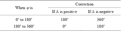
The azimuth of the sun;  is normalized from 0˚ to 360˚ by adding algebraically a correction from Table 1

shown below.

[image:2.595.57.288.671.731.2]

In the field, the horizontal angles from a line to the sun are obtained from direct and reverse (face left and face right or face I and face II pointing taken on the back- sight mark and the sun). It is suggested that repeating the odolites be used as directional instruments with one of two general measuring procedures being followed, which are: 1) A single foresight pointing on the sun for each pointing on the back-sight mark: here the sighting sequence is: direct on mark, direct on sun, reverse on sun, and reverse on mark, with times being recorded for each pointing on the sun. The two times and four horizontal circle readings constitute one set of data. An observation consists of one or more sets. A minimum of 3 sets is recommended. This procedure is similar to that of meas-

Table 1. Corrections for the normalized azimuth of the sun.

Correction When  is

If  is positive If  is negative

0˚ to 180˚

180˚ to 360˚

180˚

0

360˚

180˚

uring an angle at a traverse station using a directional theodolite. This procedure is based on the assumption that pointings on the sun are of approximately the same accuracy as pointings on the back-sight mark. The single foresight procedure imparts itself to proper procedure for incrementing the horizontal circle and micrometer set- tings on the back-sight. 2) Multiple foresights pointing on the sun for each pointing on the back-sight mark: here, the sighting sequence is: direct on mark, several direct on the sun, an equal number reverse on sun, reverse on mark, with times being recorded for each pointing on the sun. A minimum of 6 pointing (3D and 3R) on the sun is recommended. The multiple times, multiple horizontal circle readings on the sun and the two horizontal circle readings on the back-sight mark constitute one observation. The multiple foresight procedure is based on the assumption that pointings on the sun are significantly less accurate than back-sight pointings. The multiple foresight procedure allows for a greater number of pointings on the sun during a shorter time span [5].

Since a large difference usually exists between the vertical angle to the back-sight mark and the vertical angle to the sun, it is imperative that an equal number of both direct and reverse pointings be taken. This is even more important when using an objective lens filter. Also, the filter should not be removed or rotated between direct and reverse pointings on the sun. When reducing the data to compute the horizontal angles, the direct reading on the back-sight mark should always be subtracted from the direct foresight reading on the sun. Likewise, the reverse back-sight reading should always be subtracted from the reverse foresight reading, and add 360˚ if the resulting angle is negative. The vertical angle to the sun is usually larger than for typical surveying work. This increases the importance of accurately leveling the instrument. Because of this and other errors, it is recommended that observations not be made when the altitude of the sun is greater than approximately 45˚ [6].

2. Field Procedure and Data Collection

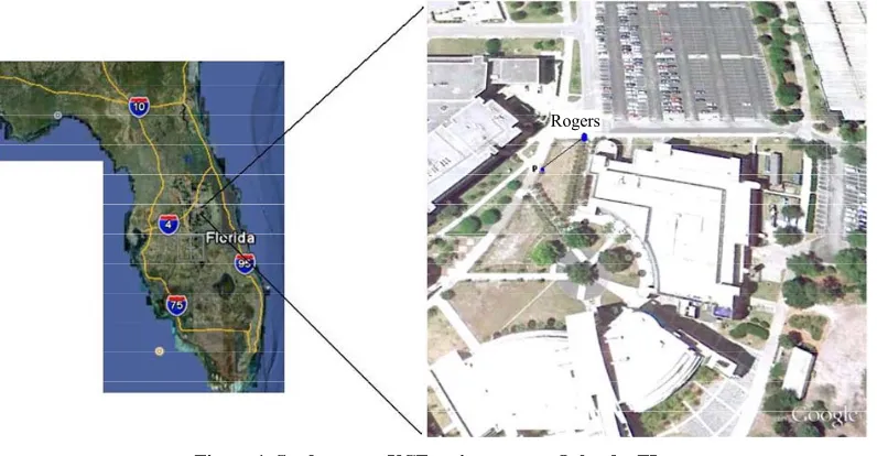
A Sun observation for azimuth field work was carried out on April 17, 2007 in a study area located in the Univer- sity of Central Florida campus in Orlando, Florida (Fig- ure 1). The geodetic coordinates of Station Rogers that

marks the beginning of the line Rogers-P as shown in the figure are (E(): 82˚22′16.82717″, N(Φ):

36˚18′00.43217″). The multiple foresight field procedure described below was used and three sets of data were collected with the telescope direct and reversed for the line in question (Table 2).

(3)

[image:3.595.102.500.88.295.2]

Rogers

Figure 1. Study area—UCF main campus, Orlando, FL.

Table 2. Sun observation for azimuth data: stopwatch readings and horizontal Circle’s readings.

Time Information (WWV) UTC: 21:48:10

DUT: –0.1 sec (stopwatch = 00:00:00)

Instrument Location Information: Latitude (): 28˚36′42″N

Latitude (): 81˚11′36″W

Observation Stopwatch reading Horizontal circle readings

Target: Direct 00˚00′00″

First-Telescope: Direct 0:18:06.30 295˚58′40″

Second-Telescope: Direct 0:19:30.21 296˚10′50″

Third-Telescope: Direct 0:21:01.50 296˚22′20″

First-Telescope: Reverse 0:23:38.05 116˚42′40″

Second-Telescope: Reverse 0:24:42.43 116˚51′10″

Third-Telescope: Reverse 0:25:14.93 116˚55′40″

Target: Reverse 179˚59′50″

the start of each minute. If one hears double clicks for the 1st, 2nd and 3rd second, for example, the DUT correction is +0.3 seconds. Up to the 8th second, each double c1ick represents a correction of +0.1 seconds. To assign a negative sign to the correction, the code is to note what is heard starting with the 9th second. If no double clicks are heard during the first 8 seconds, one must count the double clicks, if any, from the 9th second onward to determine negative DUT and the amount. For example, if the 9th, 10th, 11th and 12th clicks are doubled, the DUT correction is –0.4 seconds, each double-click representing –0.l seconds correction.

The stop watch was started at the tone of the WWV station and the “start time” was recorded. A Trimble® M3 total station with a sun filter was set up at station P which was in clear view of the sun. Then, a backsight (BS) was taken on station Rogers and the Horizontal An- gle (HA) were set to 00˚00′00″. The telescope was turned to the sun and while it is in direct (D) position, the

[image:3.595.65.540.330.497.2]

(4)

horizontal circle.

3. Field Data Manipulation and Azimuth

Computation

Below is the computations performed on the data of Ta- ble 2 in order to compute the azimuth of sun and further

azimuth of the line Rogers-P shown in Figure 1 above.

The summary of the computed values of the Sun’s local hour angle (), declination (), and azimuth () at the observation latitude () for the field data in Table 2 is

shown in Table 3.

Correction to stopwatch equals UT1 when stopwatch was started:

UTC = 21 h 48 m 10.0 s DUT= –0.1 s

UT1= 21 h 48 m 9.9 s (at stopwatch = 0:00:00)

From Table 5 (Appendix A), which shows Sun and

Polaris ephemeris on the day Sun observation was be performed:

GHA 0 h = 180˚03′32.8″ GHA 24 h = 180˚06′59.4″

Decl 0 h = 10˚15′55″ Decl 24 h = 10˚37′03.5″ Sun’ semi-diameter = 0˚15′56.1″.

3.1. First Pointing with Telescope Direct UT1 = 18 m 6.3 s + 21 h 48 m 9.9 s = 22 h 6 m 16.2 s

GHA = GHA 0 h + (GHA 24 h – GHA 0 h + 360) (UT1/24) = 180˚03′32.8″ + (180˚06′59.4″ – 180˚03′32.8″

+ 360) (22 h 6 m 16.2 s/24) = 511˚40′46.08″ = 151˚40′

46.08″

LHA = GHA – w = 151˚40′46.08″ – 81˚11′36″ = 70˚ 29′10.08″

Decl = Decl 0 h + (Decl 24 h – Decl 0 h) (UT1/24) + (0.0000395) (Decl 0 h) sin(7.5 UT1) = 10˚15′55″ + (10˚ 37′03.5″ – 10˚15′55″) (22 h 6 m 16.2 s/24) + (0.0000395) × (10˚15′ 55″) × sin(7.5 × 22 h 6 m 16.2 s) = 10˚35′23.67″

AZsun = tan 1 sin 70 29 10.08

cos 28 36 42 tan10 35 23.67 sin 28 36 42 cos 70 29 10.08

   

       



    = –89˚44′46.98″

Since LHA is between 0˚ to 180˚, and AZsun is negative, the normalized correction equals 360˚.

AZsun = 270˚15′13.02″

D Ang Rt = 295˚58′40″ – 0˚00′00.0″ = 295′58′40″

h = sin–1_(sin28_˚₃₆_′₄₂_″_sin10_˚₃₅_′_23.67_″_cos28_˚₃₆_′₄₂_″_cos 10˚35′23.67″cos70˚29′10.08″) = 22˚06′7.03″

dH = (sun’s semi-diameter)/cosh = (0˚15′56.1″)/22˚06′

7.03″ = 0˚17′11.93″

Left edge pointed D & R; therefore the correction dH is positive.

Ang Rt = R Ang Rt + dH= 295˚58′40″ + 0˚17′11.93″ = 296˚15′51.93″

AZL = AZsun + 360 – Ang Rt = 270˚15′13.02″ + 360 –

296˚15′51.93″ = 333˚59′21.09″.

3.2. Second Pointing with Telescope Direct UT1 = 19 m 30.21 s + 21 h 48 m 9.9 s = 22 h 7 m 40.11 s

+ 360) (22 h 6 m 16.2 s/24) = 512˚01′44.93″ = 152˚01′

44.93″

LHA = GHA – w = 152˚01′44.93″ – 81˚11′36″ = 70˚ 50′8.93″

Decl = Decl 0 h + (Decl 24 h – Decl 0 h) (UT1/24) + (0.0000395) (Decl 0 h) sin(7.5 UT1) = 10˚15′55″ + (10˚ 37′03.5″ – 10˚15′55″) (22 h 7 m 40.11 s/24) + (0.0000395) × (10˚15′55″) × sin(7.5 × 22 h 7 m 40.11 s) = 10˚35′24.9″

AZsun = tan 1 sin 70 50 8.93

cos 28 36 42 tan10 35 24.9 sin 28 36 42 cos 70 50 8.93

   

       



[image:4.595.59.540.596.734.2]

    = –89˚34′45.59″

Table 3. Summary of the computed values of the sun’s local hour angle (), declination (), and azimuth () at the observation latitude () for the field data in Table 1.

Latitude () Sun Declination () Local Hour Angle () Normalized Sun Azimuth ()

Observation deg min sec deg min sec deg min sec deg min sec

First-Telescope: Direct 28 36 42 10 35 23.67 70 29 10.08 270 15 30.02

Second-Telescope: Direct 28 36 42 10 35 24.90 70 50 8.93 270 25 14.41

Third-Telescope: Direct 28 36 42 10 35 26.24 71 12 58.50 270 36 07.33

First-Telescope: Reverse 28 36 42 10 35 28.53 71 52 7.13 270 54 43.63

Second-Telescope: Reverse 28 36 42 10 35 29.47 72 8 12.98 271 02 21.57

Third-Telescope: Reverse 28 36 42 10 35 29.95 72 16 20.56 271 06 12.51

(5)

AZsun = 270˚25′14.41″

D Ang Rt = 296˚10′50″ – 0˚00′00.0″ = 296˚10′50″

h = sin–1_(sin28_˚₃₆_′₄₂_″_sin10_˚₃₅_′_24.9_″_cos28_˚₃₆_′₄₂_″_cos 10˚35′24.9″cos70˚50′8.93″) = 21˚47′42.48″

42.48″ = 0˚17′9.71″

Ang Rt = R Ang Rt + dH= 296˚10′50″ + 0˚17′9.71″ = 296˚27′59.71″

AZL= AZsun + 360 – Ang Rt = 270˚25′14.41″ + 360 –

296˚27′59.71″ = 333˚57′14.7″.

3.3. Third Pointing with Telescope Direct UT1 = 21 m 1.5 s + 21 h 48 m 9.9 s = 22 h 9 m 11.4 s

+ 360) (22 h 9 m 11.4 s/24) = 512˚24′34.5″ = 152˚24′34.5″

LHA = GHA – w = 152˚24′34.5″ – 81˚11′36″ = 71˚ 12′58.5″

Decl = Decl 0 h + (Decl 24 h – Decl 0 h) (UT1/24) + (0.0000395) (Decl 0 h) sin(7.5 UT1) = 10˚15′55″ + (10˚ 37′03.5″ – 10˚15′55″) (22 h 9 m 11.4 s/24) + (0.0000395) × (10˚15′55″) × sin(7.5 × 22 h 9 m 11.4 s) = 10˚35′26.24″

AZsun = tan 1 sin 7112 58.5

cos 28 36 42 tan10 35 26.24 sin 28 36 42 cos 7112 58.5

   

       



    = –89˚23′52.71″

Since LHA is between 0˚ to 180˚, and AZsun is nega-tive, the normalized correction equals 360˚.

AZsun = 270˚36′7.33″

D Ang Rt = 296˚22′20″– 0˚00′00.0″ = 296˚22′20″

h = sin–1_(sin28_˚₃₆_′₄₂_″_sin10_˚₃₅_′_24.9_″_cos8_˚₃₆_′₄₂_″_cos10_˚ 35′24.9″cos70˚50′8.93″) = 21˚27′40.8″

40.8″ = 0˚17′7.33″

Ang Rt = R Ang Rt + dH = 296˚22′20″ + 0˚17′7.33″ = 296˚39′27.33″

AZL = AZsun + 360 – Ang Rt = 270˚25′14.41″ + 360 – 296˚39′27.33″ = 333˚56′21.09″

3.4. First Pointing with Telescope Reverse UT1 = 23 m 38.05 s +21 h 48 m 9.9 s= 22 h 11 m 49.95 s

+ 360) (22 h 11 m 49.95 s/24) = 513˚03′43.13″ = 153˚03′

43.13″

LHA = GHA – w = 153˚03′43.13″ – 81˚11′36″ = 71˚ 52′7.13″

Decl = Decl 0 h + (Decl 24 h – Decl 0 h) (UT1/24) + (0.0000395) (Decl 0 h) sin(7.5 UT1) = 10˚15′55″ + (10˚ 37′03.5″ – 10˚15′55″) (22 h 11 m 49.95 s/24) + (0.0000395) × (10˚15′55″) × sin(7.5 × 22 h 11 m 49.95 s) = 10˚35′

28.53″

AZsun = tan 1 sin 71 52 7.13

cos 28 36 42 tan10 35 28.53 sin 28 36 42 cos 71 52 7.13

   

       



    = –89˚5′16.37″

AZsun = 270˚54′43.63″

R Ang Rt = 116˚42′40″ – 179˚59′58″ = –63˚17′18″ = 296˚42′42″

h = sin–1_(sin28_˚₃₆_′₄₂_″_sin10_˚₃₅_′_28.53_″_{+ cos28}_˚₃₆_′₄₂_″ cos10˚35′28.53″cos71˚52′7.13″) = 20˚53′20.1″

dH = (sun’s semi-diameter)/cosh = (0˚15′56.1″)/cos20˚ 53′20.1″ = 0˚17′3.36″

Ang Rt = R Ang Rt + dH = 296˚42′42″+ 0˚17′3.36″ = 296˚59′45.36″

AZL = AZsun + 360 – Ang Rt = 270˚54′43.63″ + 360 – 296˚59′45.36″ = 333˚54′58.27″

3.5. Second Pointing with Telescope Reverse UT1 = 24 m 42.43 s +21 h 48 m 9.9 s = 22 h 12 m 52.33 s

+ 360) (22 h 12 m 52.33 s/24) = 513˚19′48.02″ = 153˚ 19′48.98″

LHA = GHA – w = 153˚19′48.98″ – 81˚11′36″ = 72˚ 08′12.98″

29.47″

AZsun = tan 1 sin 72 08 12.98

cos 28 36 42 tan10 35 29.47 sin 28 36 42 cos 72 08 12.98

   

       



    = –88˚57′38.43″

(6)

AZsun = 271˚2′21.57″

R Ang Rt = 116˚51′1″ – 179˚59′58″ = –63˚08′48″ = 296˚05′12″

h = sin–1_(sin28_˚₃₆_′₄₂_″_sin10_˚₃₅_′_29.47_″_{+ cos28}_˚₃₆_′₄₂_″ cos10˚35′29.47″cos72˚08′12.98″) = 20˚39′12.83″

12.83″ = 0˚17′1.77″

Ang Rt = R Ang Rt + dH = 296˚51′12″ + 0˚17′1.77″ = 297˚08′13.77″

AZL = AZsun + 360 – Ang Rt = 271˚2′21.57″ + 360 – 297˚08′13.77″ = 333˚54′7.8″.

3.6. Third Pointing with Telescope Reverse UT1 = 25 m 14.93 s +21 h 48 m 9.9 s = 22 h 13 m 24.83 s

+ 360) (22 h 13 m 24.83 s/24) = 513˚27′56.56″ = 153˚27′

56.56″

LHA = GHA – w = 153˚27′56.56″ – 81˚11′36″ = 72˚ 16′20.56″

29.95″.

AZsun = tan 1 sin 72 16 20.56

cos 28 36 42 tan10 35 29.95 sin 28 36 42 cos 72 16 20.56

   

       



    = –88˚53′47.49″

Zsun = 271˚6′12.51″

R Ang Rt = 116˚55′40″ – 179˚59′58″ = –63˚04′18″ = 296˚55′42″

h = sin–1_(sin28_˚₃₆_′₄₂_″_sin10_˚₃₅_′_9.95_″_{cos 28}_˚₃₆_′₄₂_″_cos 10˚35′9.95″cos 72˚16′20.56″) = 20˚32′5.08″

5.08″ = 0˚17′0.97″

Ang Rt = R Ang Rt + dH= 296˚55′42″ + 0˚17′0.97″ = 297˚12′42.97″

AZL = AZsun + 360 – Ang Rt = 271˚6′12.51″ + 360 – 297˚12′42.97″ = 333˚53′29.54″.

4. Adjustment of Measurements and Error

Modeling

Like all types of measurements in surveying, errors in azimuth determination are three types: systematic, mistakes, and random errors. In this study, only random errors in azimuth determination using the hour angle are addressed through modeling. Suppose we have a non- linear function written as:

 

Y a  e, e



0,₀2P1



(2)

Before we continue to solve this problem, we need to transform Equation (2) into linear form. A common way to perform this transformation is a linearization using Taylor’s series expansion. Equation (2) can be linearized in the form shown below:

 





0

0 0

a

Y a



  

  _ _      

   e (3)

where:

 

0

a  : Value of the function evaluated from

pa-rameter approximations

Y

 

0 ,



  0



: vector of the differences between value of

unknowns parameters and there approximation.

0

a



   _

  : Jacobian matrix, which represents the partial derivatives of all functions in with respect to each of the unknown variables.

Y

The higher-order term in Equation (3) can be dropped because it is very small and, therefore, the Equation (3) can be re-written as:

 





0

a

Y a e



  

0   _ _    



  (4)

Equation (4) can be rewritten in the form of Gauss- Markov model, which is:

e

 

y A , e



0,₀2P1



(5)

where:

y: Y a

 

₀ , which is s vector,

A:

0 a



   _

  , which is a matrix,  :



  ₀



, which is a vector.

The least-squares solution for Equation (5), whose the number of observations is larger than that of the unknown parameters, can be obtained by forming an

T

A PA matrix and calculating its inverse and

multiply-ing by _{A Py}T _{vector. This solution can be written as:}





1

ˆ _{N c} _APA _APy

 _  _  ₍₆₎

However, this solution requires that the inverse;



_T



1

A PA  exists, which means that the rank of A PAT

(7)

rameter is given in the form of variance/covariance matrix, which can be computed as:

 

₂ ₁ ₂



₁ 1

0 0

ˆ

D   N  A P A



 (7)

where 2 0

 is the variance of unit weight, and its residual vector is:

1

ˆ T

n

e y A _I AN A P y



(8)

where:

 

2 1 (9) 0

T D e  _PAN A

The variance of the whole adjustment is an unbiased estimate of the error of the fit can be written as follows; given that the observations are statistically independent:

2 0 ˆ T e P n m

  e



 

(10)

Since the Sun azimuth shown in Equation (1) is non- linear, it needs to be linearlized using Taylor’s series expansion as shown below [7]:









o





o o 1 1 o u u 1 1

u u u u

tan u tan u

                           (11)

where 1 is value of at ,

o tan u



o



1

tan u

o

u u   

  ,  



  _o



and  



  _o



Since 1

2

d _tan 1

dx x 1 x

 _

 , then:

1 2 1 2 1 2 u

tan u ,

1 u u tan u

1 u u and tan u

1 u               _  _      _  _ _             (12)

The partial derivatives of the function

sin u

cos tan sin cos



   

 

 with respect to the variables ,  and  are shown below:





2

u sin sin cos cos tan sin cos cos

cos tan sin cos

        _ _ _ _  _    _  (13a)









2

u sin sin tan sin cos cos

cos tan sin cos

      _ _ _ _  _   _  (13c)

Accordingly, we can obtain the following partial derivatives of with respect to ,  and  respectively:

1 tan u













1 2 2 2 2 2 2 2 tan u

sin sin cos cos tan sin cos cos

cos tan sin cos sin 1

cos tan sin cos

sin sin cos cos tan sin cos cos

cos tan sin cos sin

                                                 (14a)













1 2 2 2 2 2 2 2 tan u sin cos

cos cos tan sin cos

sin 1

cos tan sin cos

sin cos

cos cos tan sin cos sin cos

                2         _           (14b)













1 2 2 2 2 2 tan u

sin sin tan sin cos cos

cos tan sin cos

sin 1

cos tan sin cos

sin sin tan sin cos cos

cos tan sin cos sin

                                             (14c)

The values of and the partial derivatives in Equation (14) at are as follows:













o o o o 1 o u u

1 u u 1 u u 1 u u

tan u 270.72247

tan u 0.27218 tan u 0.95810 tan u 0.38863                      , , , . (15) 2 2

u sin cos

cos cos tan sin cos

 

 _ _ _ _

 _

(8)

[image:8.595.57.539.104.205.2]

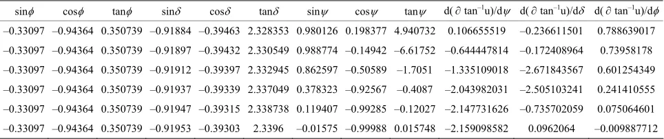
Table 4. Values of the d(tan–1u)/d, d(tan–1u)/d, and d(tan–1u)/d for the data shown in Table 2.

sin cos tan sin cos tan sin cos tan d(tan–1_u)/d__d(__tan–1_u)/d__d(__tan–1_u)/d_

–0.33097 –0.94364 0.350739 –0.91884 –0.39463 2.328353 0.980126 0.198377 4.940732 0.106655519 –0.236611501 0.788639017 –0.33097 –0.94364 0.350739 –0.91897 –0.39432 2.330549 0.988774 –0.14942 –6.61752 –0.644447814 –0.172408964 0.73958178 –0.33097 –0.94364 0.350739 –0.91912 –0.39397 2.332945 0.862597 –0.50589 –1.7051 –1.335109018 –2.671843567 0.601254349

–0.33097 –0.94364 0.350739 –0.91937 –0.39339 2.337049 0.378323 –0.92567 –0.4087 –2.043982031 –2.505103241 0.241410555 –0.33097 –0.94364 0.350739 –0.91947 –0.39315 2.338738 0.119407 –0.99285 –0.12027 –2.147731626 –0.735702059 0.075064601 –0.33097 –0.94364 0.350739 –0.91953 –0.39303 2.3396 –0.01575 –0.99988 0.015748 –2.159098582 0.0962064 –0.009887712

Table 4 shows the values of the d(tan–1u)/d,

d(tan–1_u)/d__{, and d(}__tan–1_u)/d__{for the data shown in} Table2.

This is translated into the following most probable value of the true/astronomic azimuth of the Rogers-P line in the study area: AZ = 333.93206 ± 0.20137 degrees. Re-writing Equation (11) after substituting the values

obtained in (15) yields:

5. Conclusion

270.72247 0.27218  0.38863  0.95810

       

(16) The linear error model derived in this study can be used to assess the quality of the computed sun azimuth, which is needed to determine the astronomic/true azimuth of a line at a location using the hour angle method. The error modeling framework presented in this article is essential for those seeking an improved accuracy of the estimated value of the sun azimuth. Although the model is data driven and that a little data analysis and manipulation is required to arrive at the model, the robustness of the outcome worth the efforts put forth in the process. Note that Equation (16) resembles the Gauss-Markov

model presented earlier in Equation (4). Therefore it pre- sents a linear model of the sun azimuth (Λ) derived from the data collected in the study area. The data model in- troduces the sun azimuth as a function of the random errors in the longitude and latitude of the geographic location along with that in the sun declination angle. Those errors are essential and need to be determined anyway before using them. Then the corrected value of the sun azimuth (Λ) that can be obtained using Equation (16) should be used to get the azimuth of the line in question using the procedure outlined and adopted in the calcula- tions of the line azimuth in our study area (refer to the Field Data Manipulation and Azimuth Computation sec- tion). The errors in  ,  and  , which are  ,



 and  can then be substituted in Equation (16) to compute an adjusted value of the sun azimuth (Λ) and further use that to compute corrected value of the astronomic/true azimuth of the line in question as shown in the study area.

REFERENCES

[1] P. Wolf and C. Ghilani, “Elementary Surveying: An In- troduction to Geomatics,” 10th Edition, Prentice Hall, Up- per Saddle River, 2002.

[2] J. McCormack, “Surveying,” 5th_{Edition, John Wiley and}

Sons, New York, 2004.

[3] E. Mikhail and G. Gracie, “Analysis and Adjustment of Survey Measurements,” Van Nostrand Reinhold, New York, 1982.

[4] R. Buckner, “Astronomic and Grid Azimuth,” Landmark Enterprises, Rancho Cordova, 1984.

In this study, the values of  and  have been obtained as: ±0.73241 and ±0.00071 degrees respectively using the values of the three sets of field measurements (three Direct and three Reverse) acquired in this study. The value of  was obtained independently as ±0.00344 degrees using a Topcon Hiperlite + GPS unit. Applying these values into Equation (16) above will yield the following most probable sun azimuth (Λ):

[5] J. Mackie, “The Elements of Astronomy for Surveyors,” Charles Griffin House, 1985.

[6] R. Elgin, R. D. Knowles and J. Senne, “Celestial Obser- vation Handbook and Ephemeris,” Lietz Co., Overland Park, 2000.

[7] C. Ghilani and P. Wolf, “Adjustment Computations: Spa- tial Data Analysis,” 4th Edition, John Wiley and Sons, New York, 2006.

270.72247 0.20137 degrees

(9)

[image:9.595.57.538.121.592.2]

Appendix A

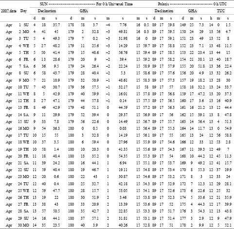
Table 5. April 2007 sun and Polaris ephemeris (Source: http://www.cadastral.com).

SUN --- For 0 h Universal Time Polaris --- 0 h UTC

Declination GHA Declination GHA TUC

2007 date Day

d m s d m s m s m s d m s d m s h m s

Apr 1 SU 4 18 35.7 178 58 3.7 –4 7.76 16 0.5 89 17 59.8 149 25 7.3 14 0 1.5 Apr 2 MO 4 41 45 179 2 32.8 –3 49.81 16 0.3 89 17 59.5 150 24 29 13 56 4.7 Apr 3 TU 5 4 49.3 179 7 0.2 –3 31.98 16 0 89 17 59.1 151 23 49 13 52 8

Apr 4 WE 5 27 48.2 179 11 25.6 –3 14.29 15 59.7 89 17 58.8 152 23 7.1 13 48 11.5 Apr 5 TH 5 50 41.4 179 15 48.6 –2 56.76 15 59.4 89 17 58.5 153 22 23.4 13 44 15 Apr 6 FR 6 13 28.6 179 20 9 –2 39.4 15 59.2 89 17 58.2 154 21 38.1 13 40 18.7

Apr 7 SA 6 36 9.5 179 24 26.4 –2 22.24 15 58.9 89 17 57.9 155 20 51.8 13 36 22.4 Apr 8 SU 6 58 43.7 179 28 40.4 –2 5.3 15 58.6 89 17 57.6 156 20 4.9 13 32 26.2 Apr 9 MO 7 21 10.9 179 32 50.9 –1 48.61 15 58.3 89 17 57.3 157 19 18.2 13 28 30 Apr 10 TU 7 43 30.7 179 36 57.5 –1 32.17 15 58 89 17 57 158 18 32.2 13 24 33.7

Apr 11 WE 8 5 42.9 179 40 59.9 –1 16.01 15 57.8 89 17 56.8 159 17 47.2 13 20 37.3 Apr 12 TH 8 27 47.1 179 44 57.8 –1 0.14 15 57.5 89 17 56.5 160 17 3.6 13 16 40.9 Apr 13 FR 8 49 42.9 179 48 51.1 0 44.59 15 57.2 89 17 56.3 161 16 21.2 13 12 44.4

Apr 14 SA 9 11 29.9 179 52 39.4 0 29.37 15 56.9 89 17 56 162 15 39.1 13 8 47.8 Apr 15 SU 9 33 7.8 179 56 22.6 0 14.49 15 56.7 89 17 55.7 163 14 56.4 13 4 51.3 Apr 16 MO 9 54 36.3 180 0 0.5 0 0.03 15 56.4 89 17 55.3 164 14 11.7 13 0 54.9

Apr 17 TU 10 15 55 180 3 32.8 0 14.19 15 56.1 89 17 55 165 13 24 12 56 58.8 Apr 18 WE 10 37 3.5 180 6 59.4 0 27.96 15 55.9 89 17 54.6 166 12 33 12 53 2.8 Apr 19 TH 10 58 1.4 180 10 20.3 0 41.35 15 55.6 89 17 54.3 167 11 39.3 12 49 7 Apr 20 FR 11 18 48.4 180 13 35.2 0 54.35 15 55.3 89 17 54 168 10 44.2 12 45 11.3

Apr 21 SA 11 39 24.2 180 16 44.1 1 6.94 15 55.1 89 17 53.7 169 9 49.2 12 41 15.7 Apr 22 SU 11 59 48.4 180 19 46.7 1 19.11 15 54.8 89 17 53.4 170 8 55.3 12 37 19.9 Apr 23 MO 12 20 0.6 180 22 43 1 30.87 15 54.6 89 17 53.2 171 8 3 12 33 24

Apr 24 TU 12 40 0.4 180 25 32.7 1 42.18 15 54.3 89 17 52.9 172 7 12.3 12 29 28.1 Apr 25 WE 12 59 47.7 180 28 15.7 1 53.05 15 54.1 89 17 52.6 173 6 22.6 12 25 32 Apr 26 TH 13 19 22 180 30 51.9 2 3.46 15 53.8 89 17 52.3 174 5 33.6 12 21 35.9