Particle Cloud Model of Electromagnetic Data in Three Dimensional Space

Particle Cloud Model of Electromagnetic Data in

Three-Dimensional Space

Huai Ding,

Science and Technology on Electronic Information Control

Laboratory

JinNiu, Chengdu, Sichuan, China No.489, Yinkang West Road

Shize Li

Science and Technology on Electronic Information Control

Laboratory

JinNiu, Chengdu, Sichuan, China No.489, Yinkang West Road

Bo Wang,

Science and Technology on Electronic Information Control

Laboratory

JinNiu, Chengdu, Sichuan, China No.489, Yinkang West Road

ABSTRACT

Data visualization is very important which transforms symbols or data into geometric figures that help researchers to comprehend the physical essence of a system especially in electromagnetic (EM) fields. In this paper, particle cloud model as a new path is introduced to depict the appearance of electromagnetic wave (EMW) which exhibits the energy value as well as the frequency of the EMW. By using such a model, the EMWs with different frequencies can be shown in one picture, making the visualization of EM data more efficient.

Keywords

Electromagnetic Data, Particle Cloud, Visualization

1.

INTRODUCTION

In Decades, data visualization as a computing method has been widely used in fields varying from physics, medicine to engineering technology with the development of computer science. It changes the method of analyzing data and makes the relationship between data and physical essence more intuitive, which as a result, facilitates one to find the hidden information. The main idea of data visualization is using specific geometrical elements such as points, lines or triangles to represent for data items. Each attribute of data can be expressed as multi-dimensional forms in order to observe them from different angles. For example, in molecular simulation, the macromolecule and protein can be constructed by sphere and rod helping researchers to discover the interesting physical process such as phase transition, clustering and crystallization, etc (1; 2; 3; 4). In fluid mechanics, different colors are adopted to stand for different fluid velocities so as to observe the hydrodynamic processes (5; 6; 7;

8).

In the field of medicine, computed tomography is generally used for disease examination by drawing the body’s inner structure with the structure information obtained by X-ray scanning (9; 10). In summary, data visualization promotes the development of science and technology and thus dramatically promotes the economic and social benefit.

In electromagnetism field, data visualization is widely studied as well. EMW is a spatial function which distributes in every corner of the space. Consequently, using lattices to divide the space into different areas is a widely used method. Generally, different values of EM energy can be expressed by the hue or depth of color. However, the draw of EMW in three-dimensional (3D) space is still an unsolved problem because the whole information of EM energy can hardly be shown in a picture in an intuitional way. Researchers use several different methods such as surface rendering, volume rendering and slice rendering to depict the EM energy. By constructing the

contour plane, surface rendering draws multi-layer objects with different colors, which represents for different energy values, to demonstrate the accurate profile of the EM energy. In Ref (11), they used marching cubes to construct the contour planes. Doi A. improves the methods and used tetrahedrons to march the energy value in order to avoid the ambiguity of marching cubes (12). After that, Octree, Interval Tree and Seed Set (13; 14; 15) _{methods are invented to improve the extract}

efficiency of volume element because the traditional method of marching cubes or marching tetrahedrals needs the calculation of every data unit which consumes lots of time. The obvious defect of surface rendering is that only the value we chose would be shown in the picture. Lots of information about EM data in the observable space are omitted. Volume rendering treats a single data as a point instead of constructing geometry element (16; 17; 18). There are two kinds of methods, one is image order and the other is object order. The most widely applied method based on image order is Ray Casting proposed by Levoy (19). It accumulates the radio energy across the whole data volume by setting the attributes of absorption and scattering of every point. Mammen invented depth-peeling algorithm based on the fragment depth sorting. Everitt

(20)

realized it on GPU with an algorithm complexity of

. Compared to surface rendering, volume rendering uses all the information of EMW to overcome the defect of surface rendering which could lead to other problems, for example, it obscures the shape of EM energy distributions. Despite various shortcomings, these methods have been used quite widely in the visualization of EM field.

However, it is always a difficult problem in the visualization of EMW that we can’t draw the EM data with different frequency and energy value at the same time because it is hard to find another element to describe frequency other than color. In this paper, it presents a particle cloud model to exhibit the different energy value and frequency. Different frequencies are drawn in different colors which is in analogy to natural light. The energy value could be exhibited by the density of particle cloud. The higher the energy is, the more dense the particle cloud is. Therefore, it solves the problem of several radios in area with different frequency. The author used the programmable shader of OpenGL (21) _{to realize the drawing}

effectively. The rest contents of the paper are organized as follows: in Model part, the author introduce the detail of this method; in Results and Discussions part it gives some results.

2.

MODEL

46 z-axis. It need to determine a rule to map the value of energy

into the number density of particles in every lattice. Firstly, a largest value and a smallest value should be set. Due to the wide dynamic range of EM energy, the author use the logarithm type of energy such as . In the rest of the paper, the superscript of is ignored and the symbol stand for the logarithmic form of energy value for convenience. The linear mapping can be expressed as:

I=kE+f (1.1)

And I is particle number.

Hypothetically, and , and the author set and ( must be larger than or equal to 0), then and . After obtaining the particle number , rounding it to the nearest integer due to integer feature of particle number, and stands for the integer. The location of each particle in a lattice should be calculated for drawing, and particle’s coordinates are generated by random distribution and read as:

c

L

r

r

 

r

r



r

(1.2)

is the central position of lattice, is random vector contains

and , is the size of lattice. The random distributions of different number density are shown in Fig 1.

Fig 1 Number density of particles from 1 to 125.

From Fig 1, the dense degree of black dots shows an apparent changing when modifying the density from 1 to 125. However, it is a problem that the difference of dense degree around the central part of Fig 1 is not very large, since this may not be advantageous for drawing because the particle densities in most of lattices belong to this range. Thus, it is necessary to increase the difference degree of this density range under fixing value of and . To achieve the goal mentioned above, the author use a controllable birth and death curve to increase the change of scope of central particle density and the relation between particle number and energy value is

 

 

off c

off c E+E E

min c

E+E E

max c

I

e

E

E

I=

I

e

E>E

a a



















(1.3)

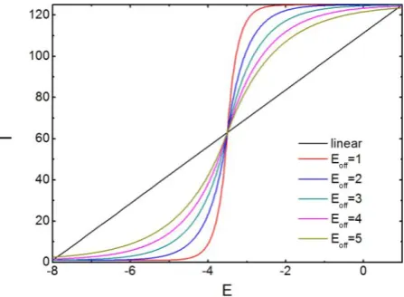
The number of particles in one lattice can be obtained by Eq.(1.3). and is the largest and smallest particle number. is the central value between and . is an offset which controls the steepness degree of curve. Parameter is





off

ln I

I

E

a





(1.4)

The curves with different have shown in Fig 2

Fig 2 The straight line correspond to linear map. The different colors represent for different .

It is found that the curve’s degree becomes very large when change from 5 to 1 and the central value of is fixed no matter what parameter it sets. The effect of particle cloud are shown in Fig 3. It displays more obvious changing trend around the central value of energy range comparing with the linear mapping especially for or 5. Therefore, the author will use this mapping parameter for drawing particle in the Result and Discussion part of paper.

Fig 3 Particle density with different . The particle density becames dense from left to right.

After that, of key importance is choosing the and which reflects the energy range of EMW one care about. Nonetheless, it may not contain all the energy values, in other words, there are some values smaller than or larger than . It is an empty lattice when based on Eq.(1.3) which may result in a big empty area if lots of are smaller than . To solve such problem, the author use Monte Carlo methods to decide whether a specified lattice has a particle. First of all, one obtain by Eq.(1.3), then generate random number which is white noise with even distribution between 0 and 1. If , one sets one particle in lattice and it is empty if .

3.

RESULTS AND DISCUSSIONS

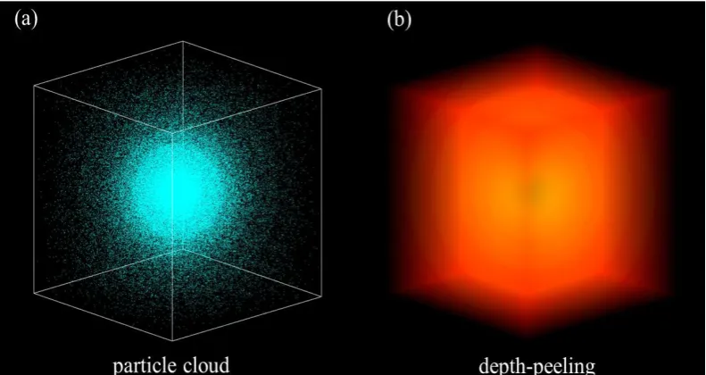
An omnidirectional source of radiation (SR) is simulated to verify the validity of particle cloud model. The SR locates at the central of a box of which size is . In this scene, there are about 150000 particles in the box which are dyed by the united color. By using the programmable shader, the rendering time is lesser than 30ms for one frame by using Intel(R) HD Graphics 530. The result is shown in Fig 4(a). From Fig 4, it is clearly found that particle density decreases gradually from the centre to the boundary of box that accord with the attenuated behavior of EMW. The feature of

omnidirectional radiation is demonstrated obviously by the symmetry of particle distribution as well. Fig 4(b) is the same scene but drawn by the depth-peeling method. Comparing particle cloud with depth-peeling, it seems that the effect of particle cloud is better than depth-peeling some way due to the exceedingly obscure image of depth-peeling. The efficiency of drawing for particle cloud model is higher than that for depth-peeling as well. Moreover, the greatest merit of particle cloud is that EMW with different frequencies could exist in one picture, which cannot be realized by surface or volume rendering.

Fig 4 (a) Particle cloud model. The white framework is the boundary. (b) Depth-peeling method. The yellow represent for a higher energy value.

The scene with size is created to verify the function that draw multi-frequencies. It is assumed that five radars, which have different work patterns and frequencies, locate randomly in this area. Radar pattern of radar I is omnidirectional radiation, frequency is 1000MHz, radar II and III and IV are directional radiation and frequencies are 2000 MHz, 3000 MHz and 4000MHz, respectively. Due to the abundance of particles, one vertex array object corresponds to one radar in our configuration which is advantageous for highly efficient draw. For instance, all the particles about radar I are packaged in a vertex array object named RadVexI.

And we give the vertex array object some attributes such as position, yellow, normal and texture. The frequency of radar I is 1000MHz, thus we use yellow color represent for 1000MHz. The normal and texture attributes are set by NULL because we treat particle as point. When using glDrawArrays(), the OpenGL launches multi-kernels of GPU to draw these particles. The RGBA of Radar I, II, III, IV are

, , , , corresponding to yellow, red, green and azure, respectively. The fourth component alpha means the transparency of vertex and alpha=1 is non-transparent.

48 The result is shown in Fig 5. The figure shows explicitly four

radars with different working frequencies which are easily distinguished by eyes. It tells us that Radar I with 1000MHz working frequency is an omnidirectional radiation because of the symmetrical distribution of points. The distribution of red, green and azure points demonstrate obviously that radar II, III and IV are directional radiation. And particle cloud model can display the direction of radiation very well. Furthermore, the energy strength of EMW at different positions are also distinguished based on the dense degree of point. Hence, one can roughly recognize the relative location of radars in box.

Nevertheless, it causes the obscure issue which makes those

particles far from camera vanish because the particles who near the camera replace the particles behind them as a result of depth test in OpenGL. This is the most common problem in the visualization of three-dimensional data. In our method, a well way to solve such a problem is that given the particle transparent attribute, the alpha of vertex is determined by the depth of particle in projected coordinate system of screen. As it is known, the z-depth range from 0 to 1, if a particles near the camera, z=0, and alpha close to 1 for particle far from camera. In the fragment shader, the alpha-component of gl_FragColor is set by z. Then, we should shutdown the depth test and open the fragment blend function which result in the effect in Fig 6 finally.

Fig 6 The transparency of particle determined by depth.

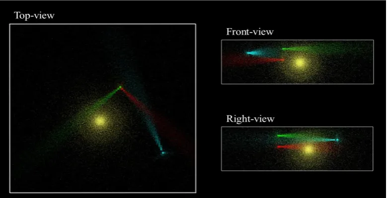
Comparing with Fig 5, it is found that the four different radars are more distinct especially for those particles far from camera. The particles behind others are still shown in the picture. In this scene, it has about 50000 particles and the rendering time is 12ms, that is to say, the refresh is 83

frame/s. It would be convenient for change of view to observe the system in different angles which is advantageous for exhibiting the EM data completely. Fig 7 shows the particle cloud from top, front and right view. From this figure, locations and radiant direction of radars are accurately told.

Fig 7 Top, front and right view of the particle cloud.

4.

CONCLUSION

We use a particle cloud model to display the energy distribution of EMW in three-dimensional space. An appropriate mapping relation between particle number density and energy value is proposed to reflect the strength of EM instead of color mapping. Color is used to distinguish the different frequencies of EMW so that the model can exhibit

prospect in electromagnetic field.

5.

ACKNOWLEDGMENTS

This work is supported by Key of Science and Technology on Electronic Information Control Laboratory.

6.

REFERENCES

[1] Jiang, H. and Ding, H. Direct sampling of multiple single-molecular rupture dominant pathways involving a multistep transition. Phys. Chem. Chem. Phys. 2014, Vol. 16, pp. 25508-25514.

[2] Tong, Hua, et al. Revealing Inherent Structure Characteristics of Jammed Particulate Packings. Phys.Rev.Lett. 2019, Vol. 122, p. 215502.

[3] Schluttig, Jakob, Korn, Christian B. and Schwarz, Ulrich S. Role of anisotropy for protein-protein encounter. Phys.Rev.E. 2010, Vol. 81, p. 030902.

[4] Woodhouse, F G and Goldstein, R E. Spontaneous circulation of confined active suspension. Phys.Rev.Lett. 2012, Vol. 109(16), p. 168105.

[5] Wioland, H., Woodhouse, F G and Dunkel, J. Confinement stabilizes a bacterial suspension into a spiral vortex. Phys.Rev.Lett. 2013, Vol. 110(26), p. 268102.

[6] Lushi, E., Wioland, H and Goldstein, R E. Fluid flows created by swimming bacteria drive self-organization in confined suspension. Proc Natl Acad Sci U S A. 2014, Vol. 111(27), pp. 9733-8.

[7] Chen, Shiyi and Doolen, Gary D. Lattice Boltzmann method for fluid flows. Annual reviews of fluid mechanics. 1998, Vol. 30, pp. 329-364.

[8] Yoshino, M., et al. A numerical method for incompressible non-Newtonian fluid flows based on the lattice Boltzmann method. Journal of Non-Newtonian Fluid Mechanics. 2007, Vol. 147, pp. 69-78.

[9] Bach, Peter B, et al. Computed tomography screening and lung cancer outcomes. JAMA. 2007, Vol. 297(9), pp. 953-961.

[10] Mayo, JR. High resolution computed tomography.Technical aspects. Radiol Clin North Am. 1991, Vol. 29(5), pp. 1043-1049.

[11] Lorensen , W. E. and Cline , H. E. . Marching Cubes:A High Resolution 3D Surfaces Construction Algorithm. Computer Graphics. 1987, Vol. 21(4), pp. 163-169. [12] Doi, A. and Koide, A. An efficient method of

triangulating euqi-valued surfaces by using tetrahedral cells. IEICE TRANSACTIONS on Information and System. 1991, Vols. E74-D(1), pp. 214-224.

[13] Wilhelms, J. and Gelder, A. V. . Octrees for faster isosurface generation. ACM Trans. Graph. 1992, Vol. 11, pp. 201-227.

[14] McCreight, E. M. . Priority search trees. SIAM J. Comput. 1985, Vol. 14, pp. 257-276.

[15] Bajaj, C. L. , Pascucci, V. and Schikore, D. R. . Fast isocontouring for improved interactivity. 1996.

[16] Govindaraju, N. K. , Lin, M. C. and Manocha, D. . Vis-Sort:Fast Visibility Ordering of 3D Geometric Primitives. s.l. : UNC-CH Technical Report, 2004. [17] Mammen, Abraham. Transparency and antialiasing

algorithms Implemented with the virtual pixel maps technique. IEEE Computer Graphics and Applications. July 1989, Vol. 9(4), pp. 43-55.

[18] Diefenbach, Paul. Pipeline Rendering:Interaction and Realism Through Hardware-Based Multi-PassRendering. Department of Computer Science, University of Pensylvania.

[19] Levoy, M. Display of surfaces from volume data. IEEE Computer Graphic and Applications. 1988, Vol. 8(3), pp. 29-37.

[20] Everitt, C. . Interactive order-independent transparency. s.l. : Santa Clara:NVIDIA Corporation, 2001.