Article
1
Benthic Habitat Morphodynamics- Using Remote
2
Sensing to Quantify Storm-Induced Changes in
3
Nearshore Bathymetry and Surface Sediment Texture
4
at Assateague National Seashore
5
Arthur Trembanis 1,*, Alimjan Abla2, Ken Haulsee 1, and Carter DuVal1
6
1 School of Marine Science and Policy
7
University of Delaware
8
Lewes, DE 19958 USA
9
10
2 Middle East Technical University
11
Institute of Marine Science, Turkey
12
Visiting PhD Fellow at UD 2016-2017
13
14
* Correspondence: [email protected]; Tel.: (+1 302-831-2498)
15
16
Abstract: This study utilizes repeated geoacoustic mapping to quantify the morphodynamic
17
response of the nearshore to storm-induced changes. The aim of this study was to quantitatively
18
map the nearshore zone of Assateague Island National Seashore (ASIS) to determine what changes
19
in bottom sediments, benthic fauna and fish habitat are attributable to storm events including
20
hurricane Sandy and the passage of hurricane Joaquin. Specifically, (1) the entire domain of the
21
National Parks Service offshore area was mapped with side-scan sonar and multibeam bathymetry
22
at a resolution comparable to that of the existing pre-storm survey, (2) a subset of the benthic stations
23
were resampled that represented all sediment strata previously identified, and (3) newly obtained
24
data were compared to that from the pre-storm survey to determined changes that could be
25
attributed to specific storms such as Sandy and Joaquin. Capturing event specific dynamics requires
26
rapid response surveys in close temporal association of the before and after period. The time-lapse
27
between the pre-storm surveys for Sandy and our study meant that only a time and storm integrated
28
signature for that storm could be obtained whereas with hurricane Joaquin we could identify
29
impacts to the habitat type and geomorphology more directly related to that particular storm. This
30
storm impacts study provides for the National Park Service direct documentation of storm-related
31
changes in sediments and marine habitats on multiple scales: from large scale, side-scan sonar maps
32
and interpretation of acoustic bottom types, to characterize as fully as possible habitats from 1 to 10
33
m up to many kilometer scales, as well as from point benthic samples within each sediment stratum
34
and these results can help guide management of the island resources.
35
Keywords: side-scan sonar, swath bathymetry, habitat monitoring, hurricane Sandy, hurricane
36
Joaquin, climate change, shoreline detection, remote sensing
37
38
1. Introduction
39
The overall goal of this study was to map the morphodynamic changes to the nearshore zone of
40
Assateague Island National Seashore (ASIS) to determine what changes in bottom sediments,
41
benthic fauna and fish habitat occurred are attributable to storm impacts such as Superstorm Sandy
42
and hurricane Joaquin. Specifically, we (1) mapped the full survey area with side-scan sonar and
43
multibeam bathymetry at a resolution comparable to that of the pre-storm survey, (2) resampled a
44
subset of the benthic stations that represented all sediment strata previously identified, and (3)
45
compared newly obtained data to that from the pre-storm survey to examine storm impacts. This
46
survey design aimed to document storm-related changes in sediments and marine habitats on
47
multiple scales: from large scale, side-scan sonar maps and interpretation of acoustic bottom types,
48
to characterize as fully as possible habitats from 1 to 10 m up to many kilometer scales, as well as
49
from point benthic samples within each sediment stratum.
50
1.1 Background on Acoustic Mapping
51
Human reliance upon, and interference with benthic ecosystems necessitates an understanding of
52
the spatial extent, structure, and function of these unique ecosystems (Balthis et al., 2006; Engle et
53
al., 2009). This project work utilized advanced geoacoustic techniques for remote benthic habitat
54
mapping and employed both traditional technologies for wide area coverage combined with point
55
sampling and robotic systems including an autonomous underwater vehicle (AUV) and a remotely
56
operated vehicle (ROV) for gathering data in an unprecedented level of resolution over targeted
57
regions of interest. Knowledge gained from this study thus allows coastal and estuary
58
environmental stakeholders responsible for the Assateague Island National Seashore (ASIS) to
59
better manage resources to protect these environments by providing information on the location of
60
habitats, species’ distributions and associations to varying sedimentary and morphological regimes.
61
The new benthic habitat and geomorphologic datasets will serve as a useful reference for an array
62
of mapping and management efforts particularly providing insights into temporal dynamics from
63
before and after storms.
64
Estuarine and coastal regions of the US face multiple marine spatial planning issues and challenges,
65
including the effects of episodic storms, climate change, and other stressors (Douvere and Ehler,
66
2005). In particular, there has been a strong interest in and multiple efforts to examine the effects of
67
hurricane Sandy on the seabed within the Mid-Atlantic Bight (Goff et al., 2013; Hapke et al., 2013;
68
Trembanis et al., 2013). The anticipated impacts of offshore development on the seabed and to the
69
ecology and, more generally, NOAA’s initiatives in marine spatial planning (Douvere and Ehler,
70
2009) point to an ever-increasing need for both base-line mapping and monitoring efforts directed
71
at biological habitats and geological features of the littoral zone.
72
In this study, we realized the need to fuse disparate data streams and recognized the most effective
73
means of analyzing and understanding them is through data visualization. By repeated benthic
74
habitat and morphology mapping, this field effort and the subsequent data analysis provides a
75
critical extension to the previous study of the ASIS site (2011-2012). We recognize that together
76
these data sets collected over multiple years represent a knowledge base much greater than the sum
77
of its parts, and it is this fact that motivated the project. The ecological services provided by these
78
benthic communities (Diaz et al., 2004), e.g., physical structure, prey species refuge and recreational
79
fisheries, justify the renewed interest in these communities and habitats.
80
Recent benthic mapping on similar prior projects to this project (Trembanis et al., 2012; Miller et al.,
81
2010; Raineault et al., 2012) have demonstrated that, in general, shallow coastal ecosystems are far
82
more complex and heterogeneous in bottom type than typically anticipated. Furthermore,
83
conventional sampling by direct methods (i.e., bottom grabs or dredges) is also generally
84
recognized as severely limited by several factors including gear bias, spatial averaging and limited
85
sample density. It is only from the careful fusion of multiple technologies (i.e., ship-based, ROV,
86
AUV, grab samples, and dredge) that one is able to compile the complete picture of the nature and
87
composition of the bottom (Diaz et al., 2004, Miller et al., 2010; Raineault et al., 2012; Raineault et al.,
88
2013).
89
Accurate bathymetric and backscatter data are essential for hydrographic charts, dredging, and
90
habitat mapping. Previously, the primary method for seafloor mapping was the use of
beam bathymetry. It is an accurate technique for collecting seafloor data, yet there are a number of
92
limitations. In single-beam surveys, a discrete footprint of the seabed is ensonified leaving large
93
gaps between adjacent survey tracks that are not surveyed. Single-beam surveys typically cover
94
only 5-10% of the total seafloor area leaving large portions unsampled. Therefore, the maps
95
generated from single-beam sonar samples may lack high-enough resolution to detect small and
96
ecologically important habitat features (Parnum et al., 2009). In a recent study, Parnum et al. (2009)
97
found that a full coverage swath sonar system resulted in a 90% classification accuracy compared to
98
70-80% accuracy from a single beam system approach. Using conventional methods like RoxAnn
99
(e.g., Hauser 2002; Wilson and Madsen, 2006), found that the sampling is limited to a single sonar
100
point footprint directly below the vessel, and maps necessitate heavy interpolation between track
101
lines. In shallow settings, single-beam systems therefore require progressively more and more
102
tightly spaced lines as the local depth decreases. In contrast, multi-beam echosounders,
103
interferometric sonar, and side-scan sonar systems characterize a wide swath on either side of the
104
survey vessel. Surfaced towed acoustic sensors suffer from positioning errors associated with the
105
ambiguity of the towfish location relative to the ship GPS. Surface vessel mounted sensors also
106
suffer from reduced resolution (larger footprint) as water depth increases. Wide swath acoustic
107
methods afford the potential of effectively mapping large areas of the seafloor at a resolution
108
appropriate for habitat mapping and correlation with biological communities. Seafloor echoes can
109
be interpreted in terms of hardness and roughness and correlated with the sediment and faunal
110
characteristics.
111
Several reviews and studies of coastal sedimentary systems (e.g., Holland et al., 2003; Trembanis et
112
al., 2004; Green et al., 2004) have repeatedly demonstrated that dramatic spatiotemporal
113
heterogeneity dominates seabed settings with respect to composition and morphology and that this
114
heterogeneity is more the norm than the exception. Further exacerbating the problem, seabed
115
heterogeneity often exists at spatial scales on the order of 1-10’s m, well below typical single-beam
116
survey spacing and gridding schemes. Understanding and being able to map this spatial
117
patchiness at sufficient coverage and resolution scales is a critical component of habitat mapping
118
efforts and an important motivation behind this project.
119
1.2 Study Design and Objectives
120
This study was designed to characterize the physical and biological components of the nearshore
121
benthic zone of Assateague Island National Seashore (ASIS), including delineations of habitat and
122
assemblage types using the CMECS system. Here “assemblage” refers to the list of resident species
123
in a particular sample or site, and “habitat” refers to the spatial context of those assemblages, as
124
defined by sedimentary characteristics like grain size or organic content. We characterized benthic
125
invertebrate assemblages and their associated sedimentary habitats by analyzing Young grab
126
samples for grain size distribution, and total organic carbon (TOC). The study methods were
127
modeled off of the 2011 ASIS benthic habitat and assemblage assessment projects undertaken by
128
Versar, Inc. (Columbia, MD) and the Maryland Geological Survey (MGS), originally contracted by
129
the National Park Service (NPS). A Natural Resource Condition Assessment undertaken by ASIS
130
and the University of Maryland (Carruthers et al. 2011) ranked the Atlantic subtidal habitats as
131
reaching 99% of their reference condition (as determined by historical observations and data), albeit
132
with very limited confidence or knowledge of indicators for the reference condition. Thus, data
133
from the assessments by Versar, Inc. and the Maryland Geological Survey serve as a crucial
pre-134
Sandy (2011) point of comparison for the possible effects of the physical stressors of hurricane
135
Sandy on sediment distribution and benthic invertebrate assemblage structure. Here we make a
136
detailed comparison of benthic assemblage patterns between the pre-Sandy (2011) and post-storm
137
surveys a central part of the study, while considering inherent interpretive constraints due to the
138
temporal scope of the project and the timing of sampling events around storms. While this project
139
was one of four simultaneous benthic mapping regimes funded by the NPS in the aftermath of
Sandy, this study covered the largest habitat area, focused on the Atlantic subtidal zone, and was
141
unique in its availability of pre-Sandy (2011) reference data.
142
The updated knowledge of benthic invertebrate assemblages at Assateague Island is intended to aid
143
NPS staff in preserving park natural resources, as well as the historical and economic value of park
144
activities. Benthic invertebrates provide ecosystem services—principally as crucial food sources for
145
shelf fisheries (Molina et al. 2014)—that are necessary for the continued success of recreational
146
fishing practices at ASIS. Benthos may also act as indicators of habitat health, since certain species
147
are known to thrive in organically enriched or polluted conditions, while others perish (Pearson
148
and Rosenberg, 1978; Pocklington and Wells, 1992 Dean, 2008).
149
In this paper we set out to: (1) provide an updated subtidal resource inventory to the National Park
150
Service by determining benthic assemblage “ensemble” metrics including abundance, diversity,
151
species richness, assemblage similarity, characteristic species, and associations with environmental
152
variables; (2) analyze pre-Sandy (2011) and post-Sandy (2014-2015) assemblages with a uniform
153
statistical approach and compared them to determine what changes occurred through the study
154
period; (3) examine inter-annual variability in bottom type and macrobenthos over a four-year
155
study to determine if any of the observed changes can likely be attributed to hurricane Sandy; (4)
156
conduct targeted acoustic mapping of areas of particular interest before and after storms to provide
157
an unprecedented higher resolution of these target locations.
158
1.3 Study Site
159
Assateague Island is a 58-km long barrier island stretching from the Ocean City inlet in Maryland,
160
down past Chincoteague Island in northern Virginia. This dynamic island is characterized by
161
barrier beach and back-bay environments that are subject to the constant eroding and re-shaping
162
forces of the Atlantic Ocean. The pre-storm and post-storm surveys of Assateague Island subtidal
163
resources discussed here include the majority of the length of the island (Figure 1). We sampled
164
benthic sediments up to 1 km offshore in accordance with the pre-storm survey and NPS
165
jurisdictions (Figure 2), whereas the USGS surveyed areas further offshore of Assateague Island.
166
Historically the nearshore subtidal habitats at ASIS are comprised mostly of fine sand, with patches
167
and swaths of mud and coarser sediments. Much of the observed heterogeneity in sediments is due
168
to the relict sediments left behind by the characteristic landward ‘rolling-over’ of barrier islands.
170
Figure 1. Pre-Sandy (2011) survey sites (n=125) sampled in October 2011 on the beach (n=15) and
171
subtidally up to 1 km offshore (n=110) of Assateague Island National Seashore, Maryland. Image
172
taken from Google Earth Pro Landsat, 2016.
173
175
Figure 2. Post-storm (n=120 grabs) sampled in October 2014 (n=60 grabs, white) and 2015 (n=60
176
grabs, yellow), up to 1 km offshore of Assateague Island National Seashore survey sites, Maryland.
177
Image taken from Google Earth Pro Landsat, 2016.
178
179
2. Materials and Methods
180
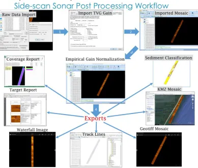
2.1. Acoustic Mapping: Side-scan Sonar Workflow
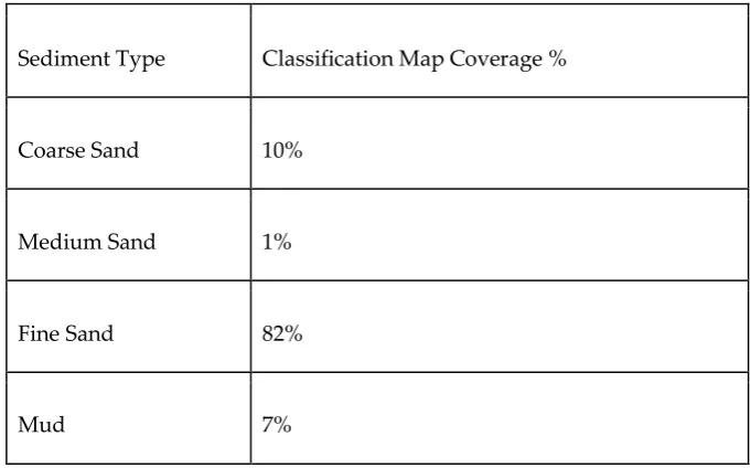
181
The side-scan sonar data collected was processed using Chesapeake Technology, Inc., SonarWiz
182
sonar processing software. Sonar data processing followed industry standard procedures for
side-183
scan data, focusing on gain corrections to remove the variation in across track brightness inherent in
184
side-scan sonar performance in order to achieve the most representative mosaic of the seafloor.
185
Standardized gain settings were chosen to make the sonar data as internally consistent as possible
186
between different daily mission datasets, while also attempting to replicate the products produced
187
from the Versar sonar data collected off Assateague in 2011. Raw Edgetech sonar files (.jsf) were
188
imported using a time-varying gain, to compensate for signal loss on the outer swath of the sonar
189
files. Once the files were imported, bottom-tracking corrections were applied if automatic bottom
190
tracking had failed. Once verified or corrected, an empirical gain normalization correction was
191
applied. This gain correction makes the data set consistent from a file-to-file basis, removing gain
192
biases caused by variations in backscatter intensity from differing sediments between each file. This
produces an interiorly consistent mosaic. From this work flow (Figure 3), several mapping products
194
were created. A standard georeferenced image file (geotiff) and Google Earth georeferenced file
195
(.kmz) are generated. Vessel navigation or track-lines files were exported as shapefiles (.shp). Each
196
gain-corrected file was exported as a waterfall image (.jpg). Target reports were generated (in .pdf
197
format), highlighting unique features or objects on the seafloor. Finally, coverage reports (.xls) list
198
the metadata for each file (start/end latitude & longitude, length, time, etc.), as well as the total area
199
and line-line overlap achieved for the complete mission.
200
201
Figure 3. Side-scan sonar post processing workflow used by the University of Delaware,
202
Assateague Island National Seashore mapping project: from EdgeTech raw data to SonarWiz to
203
shapefiles and Google Earth data products.
204
205
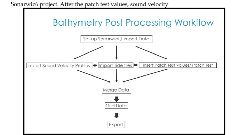
2.2. Bathy Workflow
206
The bathymetric data collected was processed using Chesapeake Technology, Inc., SonarWiz
207
sonar processing software. Sonar data processing followed industry standard procedures for
208
bathymetric data, focusing on injecting tidal offsets, sound velocity offsets, and configuring the vessel
209
files in order to achieve the most representative mosaic of the seafloor. The bathymetric processing
210
workflow (Figure 4) was standardized to keep the bathymetric representations as internally
211
consistent as possible. The first step was to configure a vessel offset file for the vessel that was
212
recording the sonar data. All of the research vessels measurements were captured including the
213
inertial measurement unit (I.M.U.) to the echosounder and the I.M.U to the antennas were recorded
214
and saved in a Sonarwiz6 vessel file. After the vessel file is created, the raw sonar data (.jsf) was
215
imported into a new Sonarwiz6 project that was set-up with an internally consistent naming
216
convention based off the date of the survey. Before the data was merged, the sound velocity profiles,
217
tide file, and the patch test values were imported into the project. After the echosounder was installed
218
and before surveying operations began, a patch test was completed to ensure that each installation
219
of the echosounder provided internally consistent data. The process accounts for offsets in roll, pitch,
220
time latency, and heading. These patch test values were then entered into the vessel offsets file. In the
221
field, sound velocity profiles were collected every hour on a Castaway CTD. The sound velocity files
(.csv) were then imported into the Sonarwiz6 project. A tide file from the days that we surveyed was
223
downloaded from NOAA Tides and Current website in the form of .csv and then imported into the
224
Sonarwiz6 project. After the patch test values, sound velocity
225
226
Figure 4. Schematic of workflow used by the University of Delaware mapping team for
227
multibeam bathymetry data from EdgeTech 6205 acquisition to gridded data products. Data collected
228
as part of a submerged mapping study for Assateague Island National Seashore in 2014-2015.
229
230
profiles, and the tide file were imported into the project, the data was merged. This merging
231
process injects all of the above information onto the XYZ point cloud that was recorded during the
232
survey to constrain the positional error, while providing the most replicable data products that are
233
internally consistent. Gridded mosaics, at a resolution of .75 meters, were then exported as a .grd file
234
using the CUBE algorithm, which is now the industry standard for providing the most accurate
235
gridded solutions. The backscatter from the bathy was also processed in Sonarwiz6 and was exported
236
as a .grd file. In all, a geotiff, .kmz, .xyz, and .grd of both the bathymetry data and the backscatter
237
data were exported as bathymetric data products.
238
2.3. Acoustic Seabed Classification Map Preparation
239
Our three, 2014-2015 acoustic surveys allowed us to make both inter and intra-annual
240
comparisons for storm-related changes in bottom sediments. The first survey resulted in side-scan
241
sonar mosaics and sediment acoustic class shapefiles from June 2014. These data include 5 side-scan
242
sonar mosaics and sediment class shapefiles that were generated from the side-scan sonar data
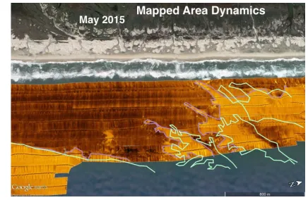
243
collected during June 20 – 25, 2014 (Figure 6 upper plot). The second survey was the most broadly
244
defined and resulted in side-scan sonar mosaics and sediment class shapefiles for May 2015 (Figure
245
8). These data include 12 side-scan sonar mosaics and sediment class shapefiles that were generated
246
from the side-scan sonar data collected during May 12 – 21, 2015.
247
Finally, we conducted a set of spot selected surveys in October 2015 producing side-scan sonar
248
mosaics and sediment class shapefiles. This survey was spatially focused on areas of change
249
following hurricane Joaquin. Data were collected during October 13 – 16, 2015.
250
2.3.2. Acoustic Seabed Classification
251
First, all the available datasets were imported into ArcGIS platform under coordinate system -
252
WGS_1984_UTM_Zone_18N. Then, manually digitized acoustic classes were matched against
side-253
scan sonar mosaics and grain size data of grab samples to make sure the side-scan sonar mosaics
254
were segmented correctly. After that, sediment class boundaries were matched between neighboring
255
sediment classes to correct any inconsistencies in the interpretation of side-scan sonar mosaics, (i.e.
256
to keep the class assignments consistent from one survey day to the next). Minor discrepancies with
257
the side-scan sonar data interpretation and inconsistencies in sediment class boundaries were
258
corrected manually using ArcGIS Edit tool.
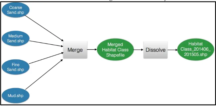
After fixing all the discrepancies related with side-scan sonar data interpretation, all the
260
same sediment classes in different shapefiles were merged into a single shapefile using the “Merge”
261
tool in Arc Toolbox (Figure 5). Overlapping areas of the same sediment classes between different
262
shapefiles were dissolved into one using the “Dissolve” tool in Arc Toolbox. At the end, 4 single
263
shapefiles representing 4 different sediment classes namely Coarse Sand, Medium Sand, Fine Sand,
264
and Mud, were merged into one single shapefile named Sediment Class_201406_201505.shp. A new
265
field named “Area” was added to the table of contents of the newly generated shapefile and areas in
266
m2were calculated for the sediment classes using “Calculate Geometry” method in ArcGIS.
267
268
Figure 5. Flow-chart of data processing steps for manually segmented side-scan sonar - sediment
269
classification into a habitat map for Assateague Island National Seashore, developed by the
270
University of Delaware 2014-2015.
271
272
The acoustic backscatter data collected in the field surveys was used to generate mosaic sonar
273
images as outlined in the section above and then digitized using ArcGIS to manually outline and
274
build categorical maps of the Assateague Island survey domain. The same acoustic class types as
275
used in the 2011 precursor study by Versar/MGS were adopted here for consistency and the previous
276
acoustic class maps were used along with the newly acquired and created side-scan sonar mosaics to
277
guide the human operator in the segmentation process. All segmentation effort was conducted by
278
the same team member for consistency and then reviewed by the principle investigator. The
279
backscatter segments were then assigned to the acoustic class and were assigned similar colors again
280
adopting the same nomenclature and color scheme as used in the precursor study to aid in
281
comparison. Note that up to this point the classes are simply acoustic classes and require some
282
external ground-truthing to further relate the classes to actual seabed types. The next step of relating
283
the acoustic classes to seabed types comes through the correlation of class maps to the benthic grab
284
samples and grain size analysis samples.
285
Figures 3 and 4 illustrate the workflows used in data processing both the side-scan sonar and
286
phase measuring bathymetric sonar.
287
2.3.3. Ground Truthing
288
Essential for any geoacoustic marine habitat mapping initiative is the need to gather ground
289
truthing observations to compare to the acoustically derived maps. Throughout our previous habitat
290
mapping campaigns we have utilized benthic grab samples for ground truthing (Raineault et al., 2012;
291
Trembanis et al., 2013). Grab samples were analyzed for grain size distribution and benthic faunal
292
composition using standard approaches (see below and references therein for details). We used a
293
modified Young grab sampler for recovering surface sediment ground truthing samples. The
294
available grain size data included grain size analysis results from 98 grab samples taken during June
295
of 2011 and 146 grab samples taken during October of 2014 and October of 2015 for benthic samples
296
plus additional ones for ground truthing only. However, only the ones taken during 2014 and 2015
297
were used to check the side-scan sonar data interpretation in this study. Additionally, a small
298
portable YSI Castaway CTD (http://www.ysi.com/castaway) was used to gather vertical profiles of
salinity, temperature, and sound speed for use in environmental characterization and swath
300
bathymetry data processing.
301
302
3. Results
303
3.1. Acoustic mapping products and findings?
304
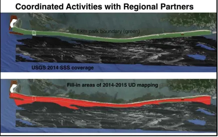
In total, over 65 km2 of geoacoustic mapping was accomplished along the entire length of
305
Assateague Island from as near to the shore as was possible out to at least 1km offshore.
306
Additional sonar lines were acquired in order to connect the nearshore ASIS park boundary to the
307
regional USGS mapping effort (Figure 6).The mapping area covered depths from 2 m-12 m
308
extending from the beach to ~2 nm offshore, with final map resolution 50 cm/pixel for side-scan
309
sonar and 1m2/pixel for bathymetry products. The field survey design as developed and agreed to
310
by all project partners conducting mapping at this and other post-Sandy NPS sites was to achieve
311
100% side-scan sonar coverage and as much bathymetric coverage as possible given the constraints
312
imposed by such shallow water survey operations. In this study we were able to achieve
313
approximately 50% swath bathy coverage (Figure 7) and 100% side-scan sonar coverage (Figure 8).
314
315
Figure 6. Overview of study site area showing park boundary (green) and recent USGS coverage
316
along with UD mapping team gap filling coverage (red).
317
319
Figure A7. Bathymetry mosaic (1m/pixel) from 2014-2015 acoustic surveys (550 kHz) for the entire
320
study area. Notable features captured in the bathymetry included pronounced shore-attached
321
oblique bars.
322
Resulting swath bathymetry data for the study side was gridded to a resolution of 1m/pixel.
323
Reliable bathymetry data was obtained for approximately half the total sonar swath width resulting
324
in 50% seafloor coverage in depths ranging from 2 to 12 m. Early sampling in 2014 around Fishing
325
Point was conducted using spacing resulting in 100% bathymetry coverage (200% side-scan sonar)
326
but the survey rate was unsustainable for the entire study site and it was agreed upon by all project
327
partners to expand the line spacing to achieve 100% side-scan and 50% bathymetry. This survey
328
strategy is also in keeping with the same approach used by the USGS in their larger regional
329
coverage provided for a meaningful connection of this study to that regional effort. The resulting
330
swath bathymetric grids extend what was only single-beam echosounder data from the precursor
331
2011 project and thus provide an enhanced baseline for AINS resource managers. Noteable
332
features captured in the bathymetry included pronounced shore-attached oblique bars.
334
Figure 8. Side-scan mosaic from 2014-2015 acoustic surveys for the entire study area.
335
A complete set of side-scan sonar mosaics with a resolution of 50 cm/pixel was generated for the
336
entire length of the island and included extensions to fill gaps between the ASIS park boundary and
337
the USGS regional survey effort. Gain settings and post-processing were set to generate an
338
internally consistent sonar backscatter map (Figure 8) that allowed for consistent segmentation and
339
interpretation with respect to sediment class. The convention used in the backscatter mosaics is for
340
bright yellow color for high-amplitude returns (i.e. coarse sand and gravel) and dark brown/black
341
for low amplitude returns (i.e. mud). Bright high-amplitude returns in the backscatter mosaic
342
were clearly associated with the raised features of shore-attached oblique sand ridges noted in the
343
bathymetry (Figure 7). Mud patches were most notable in the adjoining troughs associated with
344
the sand ridges or from relict marsh outcrops exposed by scour and barrier island migration.
345
Figure 9. Sediment classification from 2014-2015 for the entire study area. Four sediment classes
347
(Coarse and medium sand, Mud and Fine Sand) were recognized and shaded with different colors.
348
Mapping survey conducted 2014-2015.
349
As is shown in Figure 9, the sediment classification map includes four different sediment classes
350
were recognized and shaded with different colors.
351
Sediment Type Classification Map Coverage %
Coarse Sand 10%
Medium Sand 1%
Fine Sand 82%
Mud 7%
Table 1. Surficial sediment distribution by class type based on the 2014-2015 habitat mapping
352
expedition.
353
Segmentation and acoustic classification of the side-scan sonar backscatter mosaic was performed
354
via manual heads-up segmentation utilizing the same class types from the 2011 precursor study but
355
informed by the sediment grab samples collected in this study. The GIS shapefile vectors for each
356
acoustic class type are shown in Figure 9 using the same color and naming convention from 2011
357
for ease of comparison. The distribution of class type (Table 1) followed similar overall trends as
358
documented in 2011 with medium and coarse sands associated with positive relief features like the
359
large shore-attached oblique ridges and mud associated with the adjoining troughs. Notably
360
absent in the 2014-2015 data were any mappable patches of gravel. The percentage area
361
distribution of each class type are summarized in table 1.
362
The following three figures illustrate an example of an area with pronounced spatiotemporal
363
changes in acoustic class texture between the 2011 precursor map (Figure 10) and repeated surveys
364
with the EdgeTech 6205 in 2014 (Figure 11) and 2015 (Figure 12). The same backscatter amplitude
365
convention is used but the gain settings and sonar frequencies are slightly different between the
366
2011 and 2014/15 surveys. Nevertheless, the general trend shows a migration of a set of coarse
367
sand patches and the burial of a previously exposed mud patch.
369
Figure 10. Side-scan mosaic and classification shapefiles based on 2011 survey data.
370
371
372
Figure 11. May 2015 side-scan mosaic and sediment classification shapefile compared to 2011 from
373
Figure 9.
374
376
Figure 12. October 2015 side-scan mosaic and sediment classification shapefile compared to May
377
2015 (Figure 11) and 2011 (Figure 10).
378
3.2. Temporal changes in seafloor sediment type
379
Select portions of the survey domain were mapped both in May 2015 and October 2015 capturing
380
before and after the passage of hurricane Joaquin. Sediment class maps were determined in the
381
same manner and using the same grain size informed class types in order to examine changes in the
382
before and after storm surveys. Sediment types were coded from 1 to 4 from smallest to largest
383
grain size with 1 as mud, 2 as fine sand, 3 as medium sand and 4 as coarse sand and these codes
384
were manually inserted into the table of contents of sediment class shapefiles. Sediment class
385
shapefiles were then converted into raster files with sediment class type code being the value field.
386
In order to understand if the seafloor sediments are coarsening or fining from May 2015 to October
387
2015, a sediment property change map was generated by subtracting sediment class raster data of
388
May 2015 from sediment class raster data of October 2015 (Figure 13). This map shows the pattern
389
and intensity of change in sediment properties from May 2015 to October 2015 as a magnitude of
390
sediment property change index (Figure 13) . For example, positive sediment property change
391
index means the seabed became coarser, negative sediment property change index means the
392
seabed became finer and zero value means sediment property was unchanged. Higher absolute
393
value means higher intensity of change, for example +3 area represents a change from mud to
394
coarse sand -3 area represents a change from coarse sand to mud.
396
Figure 13. Sediment property change map for submerged resources of Assateague Island National
397
Seashore between May 2015 and October 2015. Positive sediment property change index means
398
seafloor became coarser, negative sediment property change index means seafloor became finer and
399
zero value means sediment texture did not change.
400
Comparison of sediment class boundaries between May 2015 and October 2015 suggest a major
401
shift (mostly south to eastward) in different sediment class boundaries. The distance of the shift in
402
the fine-coarse sediment class boundary is about 20 - 40 m in the northern portion of the study area
403
(Figure 14 and 15) and up to 80 m in the southern portion (Figures 16-19).The shift in mud-coarse
404
sediment class boundary however, was measured to be up to 180 m in the southern part (Figure 17).
406
Figure 14: Side-scan sonar mosaic interpretation, Assateague Island National Seashore, Maryland
407
(A) Side-scan sonar mosaics collected during May 13, 2015; (B) Interpretation of side-scan sonar
408
data collected in May 13, 2015; (C) Side-scan sonar mosaics collected in October 2015; (D)
409
Interpretation of side-scan sonar mosaics collected in October 2015. Note that red polygons
410
represent the same areas mapped during both May 13, 2015 and October 2015.
411
413
Figure 15: Temporal changes in sediment class boundaries, Assateague Island National Seashore,
414
Maryland. The underlying image on the bottom is the side-scan sonar mosaic collected during May
415
2015. Shaded polygons on the top represent sediment classes inferred from the side-scan sonar
416
mosaics collected during October 2015. Note the southeastward shift (18 - 50 m) in the boundary of
417
fine-coarse sand sediment classes.
418
420
Figure 16: Side-scan sonar mosaic interpretation, Assateague Island National Seashore, Maryland.
421
(A) Side-scan sonar mosaics collected during May 13, 2015; (B) Interpretation of side-scan sonar
422
data collected in May 13, 2015; (C) side-scan sonar mosaics collected in October 2015; (D)
423
Interpretation of side-scan sonar mosaics collected in October 2015. Note that red polygons
424
represent the same areas mapped during both May 13, 2015 and October 2015.
425
427
Figure 17: Temporal changes in sediment class boundaries, Assateague Island National Seashore,
428
Maryland. The profile in the bottom is the side-scan sonar mosaics collected during May 2015.
429
Shaded polygons on the top represent sediment classes inferred from the side-scan sonar mosaics
430
collected during October 2015. Please note the northward shift (180 m) in the boundary of
mud-431
coarse sand sediment class and Southeastward shift (37- 40m) in the boundary of fine - coarse sand
432
sediment class.
434
Figure 18: Side-scan sonar mosaic interpretation, Assateague Island National Seashore, Maryland.
435
(A) Side-scan sonar mosaics collected during May 14, 2015; (B) Interpretation of side-scan sonar
436
data collected in May 14, 2015; (C) Side-scan sonar mosaics collected in October 2015; (D)
437
Interpretation of side-scan sonar mosaics collected in October 2015. Note that red polygons
438
represent the same areas mapped during both May 14, 2015 and October 2015.
439
441
Figure 19: Temporal changes in sediment class boundaries, Assateague Island National Seashore,
442
Maryland. The profile in the bottom is the side-scan sonar mosaics collected during May 2015.
443
Shaded polygons on the top represent sediment classes inferred from the side-scan sonar mosaics
444
collected during October 2015. Please note the west-south-eastward shift (38 - 57 m) in the
445
boundaries of fine - coarse sand sediment classes.
446
447
3.3. Temporal changes in bathymetry
448
Storms and extreme weathering events (Morton, 2002 and Morton and Sallenger, 2003) or human
449
induced disturbances such as dredging (Cooper et al., 2007) have the potential to change the
450
nearshore bathymetry. These changes can have serious impacts to the marine flora and fauna that
451
most marine environment protection efforts are focused on.
452
The purpose of the bathymetric change comparison is to see if it is possible to determine significant
453
changes in the bathymetry after the passage of hurricane Joaquin, which passed through the area in
454
late September and early October of 2015. A total of 18 bathymetric cross sections were constructed
using Interpolate Line tool in ArcScene across areas with overlapping survey coverage from before
456
(May 2015) and after (October 2015) the passage of hurricane Joaquin. Nine of the cross sections
457
(A1, B1 to J1) were made from May 2015 bathymetry, and the other nine cross section (A2, B2 to J2)
458
were constructed from October 2015 bathymetry data along the same trackline as their pairs in May
459
2015. These bathymetry profiles were then exported as Excel spreadsheets. Sediment class type was
460
added to each of the points along the bathymetry profiles based on the attributes from the acoustic
461
sediment class maps discussed previously. Next, the Excel spreadsheets of the bathymetry profiles
462
were imported into MatLab to generate comparison charts between pairs of bathymetry profiles.
463
Sediment types were coded from 1 to 4: 1 as mud, 2 as fine sand, 3 as medium sand and 4 as coarse
464
sand. Bathymetry and sediment class comparison charts were generated by subtracting sediment
465
type values of May 2015 profiles from October 2015 profiles, in order to understand if the seafloor
466
sediments are coarsening or fining with the lateral shift in bathymetry (Figures 20 and 21).
467
468
In the areas where cross sections were constructed more or less parallel to the direction of sediment
469
class boundary shift, southwestward lateral shift of sand bars (up to 60 meters) were recognized in
470
bathymetry cross section profiles (Figures 22 and 23). In the areas where cross sections were made
471
more or less normal to the direction of sediment class boundary shift, vertical shifts of up to 65
472
centimeters are recognized (Figure 24). The largest vertical change was recognized in October 2015
473
profile J2 (Figure 24), which suggests axial incision of about 65 centimeters. This is the closest
474
profile to the shoreline. Other profiles parallel to profile J2 suggests that vertical change in
475
bathymetry seems to decrease with increasing distance from the shoreline.
476
Apart from the axial incision recognized in October 2015 profile J2 (Figure 24), comparison of May
477
and October profiles suggests that seabed changed from fairly smooth in May 2015 to incised by
478
shore oblique/perpendicular bars in October 2015(Figures 22 and 23). These are clear signs of
479
hurricane effect on the seafloor. Decrease in vertical offset towards the sea may suggest an inverse
480
relationship between hurricane effect on the seafloor and the distance from the shoreline. A
481
Comparison between bathymetry change and sediment class boundary shift in this area suggests
482
that sediments in the top of sand bars went coarser after the hurricane, while the ones in the trough
483
of sand bars went finer (Figures 20 and 21).
484
Figure 20: Bathymetry profile change versus sediment class boundary shift after Hurricane Joaquin.
486
Curved bathymetry profiles A1 (May 2015) and A2 (October 2015) are color coded according to the
487
sediment types in the chart located in the top. Horizontal scale are meter in both panels, and
488
vertical are meters in the top panel and size class index in the bottom panel. Sediment classes were
489
indexed to 4, 1 representing the finest and 4 representing the coarsest. The chart in the bottom was
490
generated by subtracting sediment type values of A1 (May 2015) from A2 (October 2015) to
491
understand if the seafloor sediments are coarsening or fining with the lateral shift in bathymetry.
492
Please note the coarsening of sediments in the top of the sand bars and fining of sediments in the
493
trough. Inset scale is in meters on both axes.
494
495
496
Figure 21: Bathymetry profile change versus sediment class boundary shift after Hurricane Joaquin,
497
Assateague Island National Seashore. Curved bathymetry profiles C1 (May 2015) and C2 (October
498
2015) in Fig. 25 are color coded according to the sediment types in the chart located in the top.
499
Horizontal scale are meters in both panels, and vertical are meters in the top panel and size class
500
index in the bottom panel. Sediment classes were indexed from 1 to 4, 1 representing the finest and
501
4 representing the coarsest. The chart in the bottom was generated by subtracting sediment type
502
values of C1 (May 2015) from C2 (October 2015) to understand if the seafloor sediments are
503
coarsening or fining with the lateral shift in bathymetry. Please note the coarsening of sediments in
504
the top of the sand bars and fining of sediments in the trough. Inset scale is in meters on both axes.
505
507
Figure 22. Bathymetry profile change after Hurricane Joaquin, Assateague Island National
508
Seashore, Maryland. Red curved line represents the bathymetry profile C1 in May 2015 and blue
509
curved line represents the bathymetry profile C2 in October 2015. Please note the Southwestward
510
lateral shift of sand bars in the bathymetry profile. Inset scale is in meters on both axes.
511
512
513
Figure 23: bathymetry profile change after Hurricane Joaquin. Red curved line represents the
514
bathymetry profile G1 in May 2015 and blue curved line represents the bathymetry profile G2 in
515
October 2015. Please note the change in surface roughness and the vertical offset in the bathymetry.
517
Figure 24: bathymetry profile change after Hurricane Joaquin. Red curved line represents the
518
bathymetry profile J1 in May 2015 and blue curved line represents the bathymetry profile J2 in
519
October 2015. Please note the axial incision in J2 profile.
520
521
Figure 25. Timeline of Storm events and seafloor mapping studies and resulting benthic habitat
522
and morphology products.
524
Figure 26. Significant wave height (Hs) in meters (m) at offshore NDBC Buoy 44009 (38.461 N 74.703
525
W) between 2011-2016 including the passage of hurricanes Sandy and Joaquin near the study site.
526
527
4. Discussion
528
This nearshore benthic morphodynamic study at Assateague Island addresses a large gap in
529
knowledge about the spatiotemporal dynamics of subtidal habitats and geomorphology in response
530
to storm events (Figure 25). This knowledge will inform subsequent general management plans to
531
best safeguard subtidal resources from anthropogenic and climate change stressors. This study also
532
provides relevant data and recommendations for future assessments at ASIS.
533
Although storms have varied morphologic impacts on different benthic substrates (i.e. coarse sand
534
versus mud), the ASIS nearshore zone experienced large lateral shifts on the order of 30 -70 m of
535
sediment type contacts resulting in changes from fine to coarse sediment type with additional
536
vertical depth changes from erosion and migration of between 50 cm to as much as 2 m associated
537
with migration of nearshore oblique sand bars as a result the passage of storms.
538
We are not able to directly link the assemblage and habitat changes outlined here to Hurricane
539
Sandy, excluding the possibility of impacts from other storms throughout the overall study period.
540
This is largely due to the study timeline (Figure 26) and constraints of sampling logistics around
541
unexpected storm events. It is more realistic to characterize the sum of assemblage differences
542
between the two surveys as integrated changes over a multi-year scale. Despite the inherent
543
uncertainty in the study, this benthic morphodynamic study is a valuable resource to inform
544
management of publicly-valued and historically under-studied habitats.
545
Author Contributions: For research articles with several authors, a short paragraph specifying their individual
546
contributions must be provided. The following statements should be used “conceptualization, X.X. and Y.Y.;
547
methodology, X.X.; software, X.X.; validation, X.X., Y.Y. and Z.Z.; formal analysis, X.X.; investigation, X.X.;
548
resources, X.X.; data curation, X.X.; writing—original draft preparation, X.X.; writing—review and editing, X.X.;
549
visualization, X.X.; supervision, X.X.; project administration, X.X.; funding acquisition, Y.Y.”,
Funding: This study was funded by the National Park Service under CESU Task P14AC00380 and modification
551
14-0001.
552
Acknowledgments: Pre-storm data was provided by Versar, Inc. We thank the Assateague Island National
553
Seashore staff and project partners for their input, including Monique Lafrance-Bartley, Bill Hulslander, Charles
554
Roman, Mark Finkbeiner, Sara Stevens and Robin Baranowski. Field and lab work was made possible by
555
Captains Kevin Beam and Evan Falgowski, Ellie Rothermel, Hannah Rusch, Danielle Ferraro, Stephanie Dohner,
556
Tim Pileguard, Trevor Metz, Anna Schutschkow, Annie Daw, Jason Button, Leah Morgan, Drew Friedrichs,
557
Rachel Dalafave, Alec Halbruner, Meghan Owings, Rachel Oidtman, and Alex Itin. We thank the
558
Environmental Protection Agency Region III’s Ocean and Dredge Disposal Program Team, especially Renee
559
Searfoss and Sherilyn Morgan Lau, for the loan of a Young grab sampler, as well as the University of Delaware’s
560
Chris Sommerfield and Adam Marsh for the loans of additional laboratory and field equipment.
561
Conflicts of Interest: The authors declare no conflict of interest. The funders had no role in the design of the
562
study; in the collection, analyses, or interpretation of data; in the writing of the manuscript, or in the decision to
563
publish the results.
566
References
567
1. Abe, Hirokazu, Genki Kobayashi, and Waka Sato-Okoshi. 2015. Impacts of the 2011 tsunami on the subtidal
568
polychaete assemblage and the following recolonization in Onagawa Bay, northeastern Japan. Marine
569
environmental research 112: 86–95. doi:10.1016/j.marenvres.2015.09.011.
570
2. Aller, Josephine Y., and Ian Stupakoff. 1996. The distribution and seasonal characteristics of benthic
571
communities on the Amazon shelf as indicators of physical processes. Continental Shelf Research 16: 717–751.
572
doi:10.1016/0278-4343(96)88778-4.
573
3. Anderson, J.R., K. J. Storey, and R. Carolane. 1981. Macrobenthic fauna and sediment data for eight estuaries on
574
the south coast of New South Wales, Technical Memorandum 81/22. Canberra.
575
4. Anderson, M.J., R.N. Gorley, and KR. Clarke. 2008. PERMANOVA+ for PRIMER: Guide to software
576
and statistical methods. Plymouth, U.K.: PRIMER-E.
577
5. Avila, L., and J. Cangialosi. 2011. Tropical Cyclone Report: Hurricane Irene (AL092011).
578
6. Avila, Lixion A. 1998. Preliminary Report: Hurricane Bonnie (AL021998). National Hurricane Center.
579
https://www.nhc.noaa.gov/data/tcr/AL021998_Bonnie.pdf
580
7. Balthis, W.L., J.L. Hyland, and D.W. Bearden. 2006. Ecosystem responses to extreme natural events: impacts
581
of three sequential hurricanes in fall 1999 on sediment quality and condition of benthic fauna in the Neuse
582
River Estuary, North Carolina. Environmental monitoring and assessment 119: 367–89.
doi:10.1007/s10661-005-583
9031-6.
584
8. Bartholomew, A. 2001. Polychaete Key for Chesapeake Bay and Coastal Virginia. Virginia Institute of
585
Marine Science. http://www.vims.edu/research/units/legacy/benthic_ecology/polychaete_key/index.php
586
9. Bender, Morris A, Thomas R Knutson, Robert E Tuleya, Joseph J Sirutis, Gabriel A Vecchi, Stephen T Garner,
587
and Isaac M Held. 2010. Modeled impact of anthropogenic warming on the frequency of intense Atlantic
588
hurricanes. Science (New York, N.Y.) 327: 454–8. doi:10.1126/science.1180568.
589
10. Berg, R. 2015. Tropical Cyclone Report: Hurricane Arthur (AL012014).
590
11. Biernbaum, Charles K. 1979. Influence of sedimentary factors on the distribution of benthic amphipods of
591
Fishers Island Sound, Connecticut. Journal of Experimental Marine Biology and Ecology 38: 201–223.
592
doi:10.1016/0022-0981(79)90068-6.
593
12. Blake, E, T Kimberlain, R Berg, J Cangialosi, and J Beven. 2013. Tropical Cyclone Report: Hurricane Sandy.
594
NOAA National Hurricane Center.
595
13. Blott, S.J., and K. Pye. 2001. Gradistat: a grain size distribution and statistics package for the analysis of
596
unconsolidated sediments. Earth Surface Processes and Landforms 26: 1237–1248.
597
14. Buttolph, A. M., W. G. Grosskopf, G. P. Bass, and N. C. Kraus. 2006. Natural sand bypassing and response
598
of ebb shoal to jetty rehabilitation, Ocean City Inlet, MD, USA. 30th Coastal Engineering Conference. San
599
Diego, CA:3,344-3,356. World Scientific Press, Singapore.
600
15. Case, R. A. 1986. Annual Summary: Atlantic Hurricane Season of 1985. Monthly Weather Review 114: 1390–
601
1405.
602
16. Carruthers, T., K. Beckert, B. Dennison, J. Thomas, T. Saxby, M. Williams, T. Fisher, J. Kumer, C. Schupp,
603
B. Sturgis, and C. Zimmerman. 2011. Assateague Island National Seashore Natural Resource Condition
604
Assessment: Maryland, Virginia. Natural Resource Report NPS/ASIS/NRR—2011/405. National Park
605
Service, Fort Collins Colorado.
606
17. Clarke, K.R. and R.N. Gorley. 2015. PRIMER v7 User Manual. Plymouth, U.K.: PRIMER-E.
607
18. Clarke, K.R. and R.N. Gorley. 2006. PRIMER v6: User manual/tutorial. PRIMER-E: Plymouth.
608
19. Clarke, K.R. and R.M. Warwick. 2001. Change in marine communities: an approach to statistical analysis
609
and interpretation. 2nd. Edition. PRIMER-E: Plymouth.
610
20. Colden, A, and R Lipcius. 2015. Lethal and Sublethal effects of sediment burial on the eastern oyster
611
Crassotrea virginica. Mar Ecol Progress Series 527: 105–117.
612
21. Dauer, Daniel M., Catherine A. Maybury, and R.Michael Ewing. 1981. Feeding behavior and general
613
ecology of several spionid polychaetes from the chesapeake bay. Journal of Experimental Marine Biology and
614
Ecology 54: 21–38. doi:10.1016/0022-0981(81)90100-3.
615
22. Diaz, Robert J, Martin Solan, and Raymond M Valente. 2004. A review of approaches for classifying benthic
616
habitats and evaluating habitat quality. Journal of environmental management 73: 165–81.
617
doi:10.1016/j.jenvman.2004.06.004.
618
23. Dittmann, Sabine, C Günther, and U Schleier. 1999. Recolonization of Tidal Flats After Disturbance. In The
619
Wadden Sea Ecosystem, ed. Sabine Dittmann, 175–192. Berlin, Heidelberg: Springer Berlin Heidelberg.
620
doi:10.1007/978-3-642-60097-5.
24. Dean, H. K. 2008. The use of polychaetes (Annelida) as indicator species of marine pollution: a review.
622
Journal of Tropical Biology 56: 11-38. http://www.redalyc.org/articulo.oa?id=44919934004
623
25. Dernie, K.M, M.J Kaiser, E.A Richardson, and R.M Warwick. 2003. Recovery of soft sediment communities
624
and habitats following physical disturbance. Journal of Experimental Marine Biology and Ecology 285-286: 415–
625
434. doi:10.1016/S0022-0981(02)00541-5.
626
26. Douvere F., and Ehler C. 2009. Ecosystem-based Marine Spatial Management: An Evolving Paradigm for
627
the Management of Coastal and Marine Places. Ocean Yearbook, Volume 23:-26
628
27. Downes, B.J., L.A. Barmuta, P.G. Fairweather, D.P. Faith, M.J. Keough, P.S. Lake, B.D. Mapstone and G.P.
629
Quinn. 2002. Monitoring Ecological Impacts. Concepts and Practice in Flowing Waters. Cambridge.
630
28. Dreyer, J, J H Bailey-Brock, and S A McCarthy. 2005. The immediate effects of Hurricane Iniki on intertidal
631
fauna on the south shore of O’ahu. Marine Environmental Research 59: 367–80.
632
doi:10.1016/j.marenvres.2004.04.006.
633
29. Engle, Virginia D, Jeffrey L Hyland, and Cynthia Cooksey. 2009. Effects of Hurricane Katrina on benthic
634
macroinvertebrate communities along the northern Gulf of Mexico coast. Environmental monitoring and
635
assessment 150: 193–209. doi:10.1007/s10661-008-0677-8.
636
30. Etter, Ron J., and J. Frederick Grassle. 1992. Patterns of species diversity in the deep sea as a function of
637
sediment particle size diversity. Nature 360: 576–578. doi:10.1038/360576a0.
638
31. Federal Geographic Data Committee. 2012. Coastal and Marine Ecological Classification Standard, June
639
2012. FGDC-STD-018-2012. Reston, VA: Federal Geographic Data Committee
640
32. Flemer, David A., Barbara F. Ruth, and Charles M. Bundrick. 2016. Effects of sediment type on
641
macrobenthic infaunal colonization of laboratory microcosms. Hydrobiologia 485. Kluwer Academic
642
Publishers: 83–96. doi:10.1023/A:1021385901210.
643
33. Fonseca, L., and Mayer, L.A., 2007. Remote estimation of surficial seafloor properties through the
644
application of Angular Range Analysis to multibeam sonar data, Marine Geophysical Researches,
645
28(2):119-126, DOI 10.1007/s11001-007-9019-4
646
34. Forrest, A.L., Trembanis, A.C., and Todd, W.L. 2012. Ocean floor mapping as a precursor for space
647
exploration. J. Ocean Tech. 7(2):71–87.
648
35. Frangipane, Gretel, Mario Pistolato, Emanuela Molinaroli, Stefano Guerzoni, and Davide Tagliapietra. 2009.
649
Comparison of loss on ignition and thermal analysis stepwise methods for determination of sedimentary
650
organic matter. Aquatic Conservation: Marine and Freshwater Ecosystems 19: 24–33. doi:10.1002/aqc.970.
651
36. Goff, John A., James A. Austin, Roger D. Flood, Beth Christensen, Cassandra M. Browne, and Steffen
652
Saustrup. 2013. Rapid Response Survey Gauges Sandy’s Impact on Seafloor. Eos, Transactions American
653
Geophysical Union 94: 337–338. doi:10.1002/2013EO390001.
654
37. Goodsell, P.J., and S.D Connell. 2005. Historical configuration of habitat influences the effects of
655
disturbance on mobile invertebrates. Mar Eco Progress Series 299: 79-87.
656
38. Gosner, Kenneth L. 1978. A Field Guide to the Atlantic Seashore: From the Bay of Fundy to Cape Hatteras. Edited
657
by R. T. Peterson. Houghton Mifflin Harcourt.
658
39. Green, M.O., Vincent, C.E., and Trembanis, A.C. 2004. Suspension of coarse and fine sand on a
wave-659
dominated shoreface, with implications for the development of rippled scour depressions. Continental
660
Shelf Research vol. 24 pp. 317-335.
661
40. Hapke, Cheryl J., Hilary F. Stockdon, William C. Schwab, and Mary K. Foley. 2013. Changing the Paradigm
662
of Response to Coastal Storms. Eos, Transactions American Geophysical Union 94: 189–190.
663
doi:10.1002/2013EO210001.
664
41. Hauser, O. 2002. Tubeworm nodule reefs of Delaware Bay: An evaluation of two acoustic survey methods
665
and lab experiments of nodule formation. University of Delaware M.S. Thesis.
666
42. Hedges, J.I., and R.G. Keil. 1995. Sedimentary organic matter preservation: an assessment and speculative
667
synthesis. Marine Chemistry 49: 81–115.
668
43. Hendrick, Vicki J, Zoë L Hutchison, and Kim S Last. 2016. Sediment Burial Intolerance of Marine
669
Macroinvertebrates. PloS one 11. Public library science, 1160 Battery Street, ste 100, San Francisco, CA 94111
670
USA: e0149114. doi:10.1371/journal.pone.0149114.
671
44. Hernández-Arana, Hector A., Ashley A. Rowden, Martin J. Attrill, Richard M. Warwick, and Gerardo
672
Gold-Bouchot. 2003. Large-scale environmental influences on the benthic macroinfauna of the southern
673
Gulf of Mexico. Estuarine, Coastal and Shelf Science 58: 825–841. doi:10.1016/S0272-7714(03)00188-4.
674
45. Holland, K.T., Keen, T., and Kaihatu, J.M. 2003. Understanding coastal dynamics in heterogeneous
675
sedimentary environments. Coastal Sediments ’03, Clearwater Beach, FL.
676
46. Hoogsteen, M. J. J., E. A. Lantinga, E. J. Bakker, J. C. J. Groot, and P. A. Tittonell. 2015. Estimating soil
677
organic carbon through loss on ignition: effects of ignition conditions and structural water loss. European
678
Journal of Soil Science 66: 320–328. doi:10.1111/ejss.12224.