Monetary policy and macroeconomic shocks in ethiopia specification, estimation and analysis of monetary policy reaction function

z

RESEARCH ARTICLE

MONETARY POLICY AND MACROECONOMIC SHOCKS IN ETHIOPIA

SPECIFICATION, ESTIMATION AND ANALYSIS OF MONETARY POLICY REACTION FUNCTION

*Dr. Zerayehu Sime Eshete

University of Nairobi, Kenya, Nairobi

ARTICLE INFO ABSTRACT

This study examines the response of monetary authority to macroeconomic shocks by employing a VECM Cointegration VAR model that considers domestic credit as the most appropriate indicator of monetary policy performance. The main findings of the study are as follows: Both net foreign asset and GDP are statistically significant and positively influence domestic credit in the long run dynamics model. It is only consumer price index that has a positive impact in the short run dynamics. All other explanatory variables negatively influence domestic credit in the short-run dynamics model. The effect of monetization of fiscal deficit on monetary policy depends on the endogeneity and exogeneity of fiscal deficits in the long run dynamics model. Moreover, the speed of adjustment or feedback effect towards long run equilibrium takes many years to make a full adjustment when there is a shock to the system. However, the speed of adjustment is inconsistent comparing with the short run dynamic analysis in this regard. The sterilization coefficient reveals incomplete sterilization activities while the offset coefficient tells us a high degree of monetary control with low degree of capital mobility. Therefore, the study recommends that the monetary authority should exercise its full discretionary power and focuses on financial sector development, secondary market and economic monetization in order to timely respond to macroeconomic shocks through market-based policy instruments.

Copyright © 2014 Dr. Zerayehu Sime Eshete, This is an open access article distributed under the Creative Commons Attribution License, which permits unrestricted use, distribution, and reproduction in any medium, provided the original work is properly cited.

INTRODUCTION

Macroeconomic stability has been an issue in heart of macroeconomics since the origin of economics. Both empirics and theories suggest that it is challenged by domestic and foreign shocks. Especially in the epoch of globalization, the unprecedented degree of economic integrations intensifies complexities and exposes domestic economy to various macroeconomic shocks (Einar, 2000). The ensuing possible turbulence is progressively severe in its nature, but they have persistent effects over time and across economic sectors in coverage. Hence, any attempts to maintain macroeconomic stability are not a simple task; rather it needs meticulous investigations in order to create a fertile ground for investment and public confidence (Jose, 2002). Macroeconomic stability in the context of the Washington Consensus is a necessary and prior condition for the achievement of all other policy goals. However, the supporters of the pro-poor economic policy reject assigning a prior condition and argue for stability must be considered as a derivative of long term economic growth, leading to thrilling debates among scholars. Such diversion from the Washington Consensus is attributed to the fact that most African countries that pursued liberalization policy had not achieved remarkable performance. For instance, their per capita income has not budged from its 20 years age even

*Corresponding author:Dr. Zerayehu Sime Eshete

University of Nairobi, Kenya, Nairobi.

though they have managed price stability. Therefore, many conclude that assigning policy rules and prior external conditionalities become a constraint on pro-poor expenditures (John and Shruti, 2007). Such policy shift has also its own implications for the monetary policy reaction function to macroeconomic shocks.

The Ethiopian economy in this regard can be an interesting case study as the current government came into power in 1991, after toppling out the socialist regime, introduced a serious economic reform program of the IMF and WB. Accordingly, the Monetary Authority has attempted to conduct basic financial liberalization program step by step including establishments of indirect or market-based policy instruments: inter-banks money markets, a treasury bills auction market as a stepping stone for open market operation, lifting up ceiling interest rates restriction and a dramatically depreciating exchange rate. However, the monetary policy shift in responding to macroeconomic shocks is challenged mainly by its weak controllability over macroeconomic variables, attributing to the existed limited financial instruments in particular and the less monetized economy in general. For instance, credit facilities and inter-bank money market could not be exercised as expected. Moreover, the Monetary Authority loses its controlling power of imposition over commercial banks’ credit and interest rates (Equare, 1994 and Haile, 2001).

ISSN: 0975-833X

Available online at http://www.journalcra.com

International Journal of Current Research

Vol. 6, Issue, 02, pp.5123-5135, February,2014

INTERNATIONAL JOURNAL OF CURRENT RESEARCH

Article History:

Received 24th

November, 2013 Received in revised form

17th

December, 2013

Accepted 19th

January, 2014

Published online 21st

February,2014

Key words:

Therefore, the study critically investigates the following research questions regarding problems associated with monetary policy and its response to macroeconomic shocks when the Bank attempts to meet its long run and short run policy objectives: What are the significant determinants of monetary policy after financial liberalization program introduced? To what extent does the effectiveness of monetary policy depend on lag structures? In the absence of broad and active financial markets as well as the lack of latitude to engage in discretionary ways, how has the Monetary Authority of Ethiopia really responded? Is there a systematic fashion in responding to macroeconomic shocks? In this regard, what policy fashion does become dominant: stabilizing or accommodating or a mixture of two? By considering these research questions, the major objective of the study is to examine the performance of the Monetary Authority of Ethiopia in responding to macroeconomic shocks since the onset of market oriented economy. The study employs a VECM Cointegration VAR model in order to address the monetary policy reaction function.

The Ethiopian Monetary Policy Performance at a Glance

Since the onset of more of market-oriented economic policy in 1991, the Monetary Authority has been implementing a wide array of economic reforms in the context of political economy. Monetary and Banking Proclamation of 1994 established the Monetary Authority as a judicial entity, separated from the governments and allowed private banks and insurance companies to operate in the industry. Monetary and Banking proclamation No 83/1994 and the Licensing and Supervision of Banking Business No. 84/1994 laid down the legal basis for investment in the banking sector. However, foreigners are prohibited from investing in the banking and insurance sectors (MOFED, 1998). An inter-bank-money market, lifting up restriction on the ceiling interest rate, devaluation of the exchange rate, and auction-based exchange rate system was introduced (NBE, 1995). Increasing the growth rate of monetary base along with the growth rate of nominal GDP is the immediate strategy to contain inflationary tendencies and maintaining external balances (NBE: 2004). The slipping away of direct control power on money supply and the growing up of the private sector paves a way to the indirect controlling mechanism of money supply. Reserve requirement in this regard is worth mentioning as the Authority set 5 percent of the net deposit of commercial banks over the period 1991 to 2005 to control the liquidity position of banks by varying the rate according with the targeted level. Note that the commercial banks’ assets in the Authority do not earn interest but their liability bears interest. However, the Authority is not able to influence commercial banks’ credit grant and money creation capacity as banks have been in excess liquidity position. The introduction of the treasury bills market was also in action in 1995 as a first stepping stone for full-fledged open market operation. This in intended to boost the Authority’s controlling power on money stock and interest rate. However, it is hard to attract private bidders so that the market is rather dominated by the Commercial bank of Ethiopia (CBE), the largest and government owned bank. This is attributed to the over liquid positions that commercial banks hold and the lower interest rate of treasury bill as compared to deposit interest rate.

Therefore, private sectors prefer bank deposits (Gazena, 2001 and Equare, 1994). The Treasury bill interest rate is not useful to determine other interest rates in Ethiopian economy. Contrary to its monetary objective, the government utilizes Treasury bill as a means of government deficit financing and causes an inflationary situation as the excess liquid absorbed is re-injected into the economy. The Monetary Authority in this regard has limited power to affect the volume of sales of the treasury due to political influence. On top of this, even the introduction of discount window facility in 2001 did not entertain any transaction through 2005 on account of excess liquidity in commercial banks.

The Monetary Authority of Ethiopia, therefore, has also encountered a problem of time lags between setting the targets and its operation attributed to the imperfectability in given market and uncertainty about demand, supply, price and the stability of political sphere. Moreover, causation factors like the absence of strong supervision and regulation, lack of independence, limited financial development, inexistence of secondary markets, and thin financial markets are responsible for the poor performance of monetary policy. Unlike developed countries that conduct explicit way of responding to macroeconomic shocks, the Ethiopian Monetary Authority has implicitly responded in some fashionable patterns that demands a thorough investigation. Note that the presence of stringent credit policy on one hand, and the absence of adequate enough absorptive capacity of the economy forced commercial banks not to lend a huge amount of credit. This left them with the saddle of excess liquid cash, leading to idle loanable fund.

Theoretical Framework

investments. However, during an economic depression, Keynesians prefer a fiscal policy to manage macroeconomic shocks. The classical school does not identify the source of extra money in an economy while Keynes identified sources such as open market operation, increased exports and deficit expenditure.

Unlike Keynesian, Friedman advocates a free market and considers that active fiscal policy is not only unnecessary, but actually harmful, worsening the very economic instability. He does not deal with fluctuations in output, employment, money income or the price level. He recommends monetary authority to be a primer in responding macroeconomic shocks. Similar to quantity theorists, the monetarists believe that the monetary authority is responsible for money that plays a significant role in economic fluctuations, particularly income and price levels (Friedman, 1968 and 1970). In summary, the response of monetary authority to change in money supply depends on macroeconomic shocks emanated from policy and non-policy shocks, monetary phenomenon and the non - monetary phenomenon as well as domestic shocks and foreign shocks (Joyce, 1991). Empirics also tell us that the change in monetary base and authority targets also one of potential sources of macroeconomic shocks. An unexpected change in the determinants and components of monetary base leads to macroeconomic instability. Annual change in monetary aggregate, instead of their absolute magnitude, is a crucial indicator of the overall macroeconomic stability (MOFED, 1999). However, targeting monetary aggregates may not be efficient as the monetary authority indirectly determines the long run inflation by determining the long run growth of money supply in the face of the quantity theory of money. This is mainly attributed to what measures the money supply- M1, M2 and M3. On the other hand, other economists provide an alternative monetary policy targeting inflation directly in the face of the difficulties encountered by the authority when it targets monetary aggregates (Sylvanus, 2004). On top of this, macroeconomic stability can be distorted by shocks from balance of payment. The monetary view of the Balance of Payment points out transactions recorded in the BOP is essentially a reflection of monetary phenomena, capturing the adjustment of actual money balances to desired levels. This means that the only transactions below the line influence domestic and foreign monetary bases and thus on domestic and foreign money supplies (Thomas and John, 1980). According to this theory, any BOP disequilibria or exchange rate movement reflects a disparity between actual and desired money balances and will automatically correct itself depending on the types of exchange rate regimes (Daniel and Van Hoose, 2000). This entails that rate fluctuation in foreign exchange is another source of macroeconomic shocks, linking the domestic economy with the rest of the world (Hallowed and MacDonald: 1989).

Considering the structure of developing countries, the experience also indicates that the primary obligation of the many monetary authorities is to finance the government budget shocks in the absence of broad and active financial markets. Under these circumstances, monetary growth depends primarily upon fiscal policy shocks by borrowing from the public via bond, running down foreign exchange reserve, and

printing money. These in turn have implications on the macroeconomic performance in general and exchange rate in particular. Moreover, inflation rate shocks can also be emerged due to excessive public deficit financings (Sylvanus, 2004). As most of the developing countries characterized by recurrent droughts, civil wars, natural disasters, and erratic rainfalls, the real sector shock also claims the response of monetary policy. Besides, supply side bottlenecks associated with the inherent production capacity of the economy has put the aggregate supply behind the aggregate demand, lead to inflation and sometimes exposes them to unplanned imports to fill domestic production gaps and food aids. This by itself leaves the countries dependant on foreign assistance when the problem is recurrent and persistent. On the other hand, Clarida, Galí, and Gertler, (2000) in their paper indicate that the major sources of macroeconomic shocks account for shifts in monetary policy. However, others contest this conclusion and rather claim shocks in investment as the main trigger factor of macroeconomic fluctuations in many developing countries (Fisher, 2006 Justiniano et al., 2008).

Empirical Literature Review

Philippine Central Bank attempts to specify a monetary policy reaction function in the context of the inflation-targeting framework. Moreover, currency stability and expansionary money supply growth are another concern of the Bank. Since January 2000, the Monetary Board has undertaken inflation-targeting framework and used a model of inter-bank lending rate for overnight loans as a policy variable in a forward-looking model to influence inflation depending upon the deviation of expected inflation from target and the expected output from trend output (John, 2004). In Turkey, Central Bank developed a reaction function by using the interaction between domestic credit and net foreign assets. In such a way that it can determine the offset and sterilization coefficients of the central bank, which could be useful in terms of measuring the scope and the stance of the monetary policy. Additionally, it is important to know the degree of relation between the Central Bank’s reaction function and the macro variables. The offset and sterilization coefficients, together with monetary policy reaction to inflation itself, measure the extent to which, monetary policy is accommodating or used systematically for monetary control (Olcay and Almila, 2000). In a case of Mexico, Korea, India, and Zambia1, in the absence of broad and active financial markets, the primary obligation of the monetary authorities was to finance the government budget. Under these circumstances, monetary growth depends primarily upon fiscal policy. Accordingly, Central Banks responded using the holding of domestic credit assets as the most appropriate indicators of monetary policy, and the variables like foreign reserves, exchange rate, real output gap, and inflation have been taken as determinants of monetary policy. The estimation of a monetary policy reaction function revealed accommodative policies (Joyce, 1991). Regarding the monetary policy reaction function for Taiwan, it's based on an extended Taylor rule, including the exchange rate, the stock’s price, and the lagged interest rate. Two major monetary policy

1

The study covers for the period: Mexico, 1959-1981;South Korea, 1962-1979; India, 1960-1971 and Zambia, 1976-1983

instruments like the discount rate and the collateral loan rate are considered, in which the discount rate or the collateral loan rate responds positively to a shock to the inflation gap and the stock price gap but does not react significantly to a shock to the output gap or the exchange-rate gap. Furthermore, except for the lagged interest rate, the inflation gap is more influential in explaining the variance of the interest rates than other endogenous variables, suggesting that the major focus of the monetary policy in Taiwan was to contain inflation in an efficient way (Chang: 2000).

Finally, in the case of Bank of Ghana, it has succeeded in reducing the gap between official and parallel exchange rates and partially succeeded in correcting the over/under valuation of nominal exchange rate by implementing various exchange rate regimes. The major instruments of monetary policy in Ghana have been the open market operation and liquidity ratios, credit ceiling and reserve requirement and bank rate. The growth rate in the money supply can be traced to rapid growth net domestic and foreign assets. Hence the bank had tried to follow a consistent lending policy in accordance with the exchange rate intervention policy and follow a consistent sterilization through an open market operations’ policy with respect to nominal exchange (Vijay, 2003).

MATERIALS AND METHODS

To investigate the response of the Monetary Authority of Ethiopia to macroeconomic shocks, the study employs an econometric analysis of VAR co-integrated model using quarterly data over the period 1991 to 2005. By taking the prevailing situations in domestic economy, the model put forth no need of restriction on the variables as exogenous and endogenous with which the study blends Johnson (1995) procedure of cointegration and error correction techniques to estimate long-and short-run coefficients. The Model specification2 considers the demand standard rule, Flow of Fund model and Taylor rule in order to specify the reaction function of monetary policy. However, interest rates in Ethiopia are not adjusted in a discretionary manner and lose its power to influence macroeconomic performance. Other monetary aggregates are also subject to uncontrollable. The extended and modified Taylor Rule(Chang, 2000) is in a better position with respect to the two major determinants of broad money supply namely domestic credit and net foreign assets. However, managing net foreign assets are mostly outside the span of control of the Monetary Authority of Ethiopia. Hence money supply management can be done only through controlling domestic assets to achieve both stabilization and balance of payment objectives. So, the change in the central bank’s holdings of domestic credit assets is chosen as the most appropriate indicator of monetary policy (Joyce, 1991). Moreover, the domestic factor that monetary growth depends primarily upon fiscal policy in developing countries for monetization of the fiscal gap (Fg) is incorporated in the

2

It is based on the formulation undertaken by Chang (2000), International Journal OF Applied Econ. 2(1), March 2000.PP.50-61) and Joyce (1991), World development Journal, vol.19, No.6, PP709-709, 1991)

model. The openness of the economy will determine the level of imported interventions, partly claims monetary policy in a way that the Central Bank possibly acts to offset or sterilize the imported effect along with exchange rate moves as well as to assess the effect of the international position and competitiveness of the country. In this regard, real effective exchange rate (REER) is recommended in place of simply exchange rate. Therefore, the final model can be written as follows:

DCt= 0 + 1 (CPIt) + 2 (GDPt) + 3 (Fgt) + 4 (NFAt) + 5

(REERt)

Whereas DCt stands for Domestic credit, NFAt stands for net

foreign assets, CPIt denotes Consumer price index, GDPt

designatesReal GDP, REERstands for Real effective exchange rate, and Fgt denotes Fiscal gap. Theories and empirical

suggest two alternative hypotheses: under a policy directed toward accommodation, the coefficients take the following signs: 1 (0, 2 0, 3 (0, 4 0 and 5 (0 while the strict

stabilization policy would place the following constraints on the coefficients: 1 (0, 2 (0, 3 (0, 4 0,5 (0. An important issue

in Econometrics is the need to integrate short-run dynamics with long-run equilibria. The analysis of short-run dynamics is

often done by eliminating trends in the variables, usually by differencing. This procedure, however, throws away potential valuable information about long-run relationships. The theory of Co-integrated VAR developed by Engle and Granger addresses this issue of integrated short-run dynamics with long-run equilibria. Therefore, the paper finally employs a Cointegrated VAR model with Error correction model (ECM).

All data all are obtained from the Central Bank of Ethiopia, Ministry of Finance and Economic Development, and International Finance Statistics of the IMF. In order to make a quantitative assessment of the competitiveness of the Ethiopian export to the rest of the world, the study constructs the real effective exchange rate index as presented annex III. Pertaining to GDP, it is not available in quarterly series. Therefore, Haile (2001) tried to study the behavior of the seasonality function of each sector in its contribution to annual GDP based on seasonality adjustment coefficients. Yimserech (2005) generated quarterly GDP from annual GDP by interpolation of either nominal or real GDP using a technique suggested by Goldstein and Khan (1976). Others also attempted to generate based on a technique from Ichero Otani and studied the quarterly contributions of each sector and came up with a seasonality adjustment coefficient for each sector and finally disaggregates using the moving average method. By comparing each of them with the prevailing condition of the country, we conduct the method of disaggregating like What Haile did (Annex II).

Econometric Results and Analysis

spurious estimation outcome: - Unit roots Test and Co-Integration Analysis.

Unit root test

The formal test for the existence of stationary is to find out if a time series contains a unit root using Dickey-Fuller (DF) and Augmented Dickey-Fuller (ADF) test. The study picks the ADF test considering the modifications on DF test made by Said and Dickey (1984) and Phillips (1987) when the error term, et is not white noise. The study conducts it with three

options:

A random walk without drift:  yt = yt-1+

1

k

j



A random walk with drift:  yt =1 + yt-1+

1

k

j



A random walk with drift around a stochastic trend:  yt=1

+2t +  yt-1+

1

k

j



We transformed the variables into natural logarithms to order to make the interpretation of coefficients in elasticity concept. As presented in Table 1, it is only variable LFg that is stationary in level, indicating a mixture of I(1) and I(0) in level form. However, all variables being studied are stationary when they are differenced once in all the three alternative formulations.

Co-Integration analysis

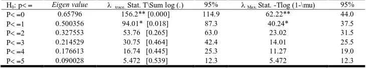
The theory of co-integration considers both short-run dynamics and long-run equilibria. The Johansen procedure in this regard is preferable, and considers maximum likelihood estimation that helps to relax the assumption of one Co integrating vector and avoids the use of two-step estimationof Engle and Granger two-stage test. Considering this, the study finds that the optimal lag length is 4 based on the basis of general to specific procedure. Having specified VAR model, Table 2 gives the optimal order of co-integration vectors based on lambda-max test and trace statistics.

* Indicates Statistical Significance at 5% and ** at 1%, if any. The test is done using PC GIVE and PCFMIL.

Diagnostic Test:

Vector portmanteau 7 lags= 234.5

Vector AR 1-4 F (144, 25) = 1.288 [0.2339] Vector normality Chi^2(12) = 62.183 [0.0000] ** Vector hetero test: Chi^2(546) = 541.77 [0.5431]

The results indicate that there are two co-integrating vectors in the system as both statistics report with their respective magnitudes greater than the critical values at 1% and 5%. Regarding to diagnostic tests, there is no problem of auto correlation, and heteroskedasticity, but it indicates a vector normalityy problems. However econometric theory states that the existence of normality problem does not affect and distort the estimators’ BLUE and consistency property, because the

Table 1. Unit Root Test using ADF procedure

Variables Without drift and Trend With drift With drift and Trend

I(0) I(1) I(0) I(0) I(0) I(1)

LDC 4.2897 -2.6646** 0.4368 -4.2883** -1.7847 -4.2993**

LNFA 1.6919 -7.6136** -6.4286** -8.2689** -6.0156** -8.8599**

LCPI 1.7081 -6.9607** -2.6861 -7.6812** -4.4635** -7.5449**

LFg -3.5956** -9.1218** -3.7114** -9.0777** -4.2410** -9.0064**

LREER -0.66180 -6.1579** -1.9858 -6.2317** -2.0478 -6.4538**

LGDP 0.42775 -19.177** -2.8925 -19.597** -15.731** -19.434**

Critical values 5%=-1.946 1%=-2.603 5%=-2.912 1%=-3.546 5%=-3.488 1%=-4.122

Source: - Estimation based on ADF test

N.B: - Graphical presentation for stationarity of the variables is presented at annex I.

Table 2. Co integration analysis and testing for co integration rank r

H0: p Eigen value  trace. Stat. T\Sum log (.) 95%  Max. Stat. -Tlog (1-\mu) 95%

P0 0.65796 156.2** [0.000] 114.9 62.22** 44.0

P1 0.500356 94.01* [0.018] 87.3 40.24* 37.5

P2 0.327553 53.76 [0.265] 63.0 23.02 31.5

P3 0.214529 30.75 [0.464] 42.4 14.01 25.5

P4 0.176613 16.74 [0.445] 25.3 11.27 19.0

P5 0.090028 5.472 [0.539] 12.3 5.472 12.3

Source: - Estimation Results based on Johansen Procedure

Table 3. Unrestricted standardized Eigenvectors’

Eigenvectors’ LDC LNFA LCPI LREER LDGP LFg Trend

’1  1.000 0.0217 0.325 0.0287 -1.411 -0.3045 0.000

(res) (1.2) (1.65) (2.54) (-7.452 (-5.35) (res)

’2  0.000 1.0000 -5.067 1.745 3.765 1.7000 -0.104

(res) (res) (-4.04) (4.83) (2.64) (9.09) (-6.25)

Source: - Estimation results of unrestricted standardized eigenvectors’

N. B: - t-value presented in the parentheses.’S shows long run elasticities as they are in logarithms form.

main purpose of normality tests is for testing hypothesis about the population parameter using the confidence interval (Enders, 1995). Therefore the inexistence of vector normality in our model doesn’t affect the coefficients and t- values. If the sample size gets larger and larger, we can easily remove the normality problem and the distribution approaches normal. The existence of two co-integrating vectors implies that there are two long run relations/equilibrium points in the system, which can be directly added into the short run equation after netting out the exogeneity problem (Badawi, 2004 and Doornik and Hendry, 2001)

Unrestricted Long Run Elasticities and Loading Coefficient

Once the rank of long run matrix identified, which is P=2, we obtain the two cointegrating vectors as the first two rows of the Eigen vector, ß matrix (long run coefficient) and the first two columns of the (matrix (speed of adjustment matrix). But, to have unique co-integration relations, we remove the trend from the first co- integrating vector and ß2t from the second

co-integrating vectors (Doornik and Hendry, 2001 and Badawi, 2004). Note that the restricted variables are ß11=1, ß17=0,

ß21=0, ß22=1 in ß's matrix. Therefore, the unique co-integrating

vector ß'sand 's results are reported below. The unrestricted standardized eigenvectors (’indicate that the first two rows of the Eigenvector of ß matrix (long run coefficient) inlong run matrix =CB’, namely the basic determinants of broad money supply namely domestic credit and net foreign assets. On top of this, Table 4 gives the unrestricted standardized adjustment coefficients. Regarding to (matrix, our interest is the first row of the (speed of adjustment matrix) in the long run matrix in unrestricted models, characterized by dominant long run feedback effect of those variables whose coefficients are relatively higher: LREER, LFg, LNFA, LCPI, LGDP and LDC in descending order with statistically insignificant of LFg.

Test for Long Run Weak Exogeneity

The values of adjustment coefficients with their respective t value give some information about weak exogeneity to domestic credit vector. Taking both adjustment coefficients and t-value into account simultaneously, we suspect that LFg would surely be exogenous to LDC due to its very low t-value. But, the formal test whether there is weak exogeneity or not, can be conducted using likelihood ratios chi^2 and to identify endogenous and exogenous variables in the model. Table 5 gives the result of testing for Long-Run Weak Exogeneity. Associated likelihood ratios, Table 5 report indicates that only LFg is weakly exogenous to the domestic credit vector while others rejected the null hypothesis that states variable is exogenous. This implies that fiscal gap is exogenous to the domestic credit vector.

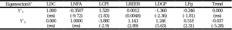
Restricted long-Run Elasticities and Loading Coefficients:

Using the information about weak exogeneity of LFg and preserving the rank of 2, the VAR system putting restriction on

's of LFg equal to zero. This is very important to netting out the adjustment coefficient of LFg due to its exogenous nature to the domestic credit, LDC and enables us to compare the result of unrestricted and restricted models (Badawi, 2004). Results of the restricted model reported in Table 6. Comparing results of restricted from unrestricted models, the magnitude of

1 for LNFA, LCPI, LREER and LFg have changed

significantly, with no change in their respective signs except LNFA. These relationships indicate that the exogeneity of LFg has great importance for relation between LDC and LNFA, LCPS, LREER. However, LGDP remains to be significant in explaining long run LDC in both restricted and unrestricted models, suggesting all variables’ signs shown that the Monetary Authority followed a mixture of both stabilization and accommodation policy. Both LNFA and LGDP have significant long run relation with positive effect. LREER is completely statistically insignificant to explain the long run

Table 4. Unrestricted standardized adjustment coefficient 

Adjustment coefficient LDC LNFA LCPI LREER LDGP LFg

1 0.0066 0.4897 0.1170 -1.1307 -0.3924 -0.5886

(1.72) (1.68) (2.41) (-3.53) (-2.69) (0.32)

2  -0.0047 0.509 0.0432 -0.1570 -0.0772 -1.1327

(-1.23) (1.58) (2.86) (-2.08) (-2.75) (-3.10)

Source: - Estimation Results of Unrestricted standardized adjustment coefficient 

Table 5. Tests for Long-Run Weak Exogeneity (H0: Variables is exogenous to DC)

Variable Chi^2 F-probability Decision over H0 Inference

LNFA 1.6772 [0.0195]** Rejection Not Exogenous

LCPI 3.8446 [0.0499]** Rejection Not Exogenous

LREER 7.9688 [0.0048]** Rejection Not Exogenous

LGDP 8.6526 [0.0033]** Rejection Not Exogenous

LFDg 0.62678 [0.4285] Acceptance Exogenous

Source: - Estimation Results for Long-run weak exogeneity

Table 6. Restricted standardized Eigenvectors’

Eigenvectors’ LDC LNFA LCPI LREER LDGP LFg Trend

’1 1.000 -0.3507 1.520 0.0012 -1.360 -0.246 0.000

(res) (-9.72) (1.83) (0.0048) (-2.36) (-1.81) (res)

’2 0.000 1.0000 -3.880 1.143 1.246 0.518 -0.037

(res) (res) (-2.9) (2.89) (5.63) (2.31) (-5.28)

relation with LDC. On the other hand, the restricted standardized adjustment coefficients are presented as follows in Table 7.

Diagnostic Test:

Vector Portmanteau (7): 225.379

Vector Normality test: Chi^2(12)= 84.463 [0.0000]** Vector hetero test: Chi^2(1050)= 1066.4 [0.3552]

As the Monetary Authority reacts to, 1(=0.02072) for LDC

indicates the speed of adjustment of feedback effects towards the long run equilibrium is 2.072 percent per quarter and 8.288 percent per annum. At this pace the adjustment towards long run equilibrium takes many years for full adjustment, this indicates how hard the response of the Monetary Authority to macroeconomic shocks.

Vector Error Correction Model

Determination of the coefficient of short-run dynamics is conducted by estimation of parsimonious VECM after the determination of long-run relationships. It is very important to specify how short run adjustment of macroeconomic variables is took place, and a fertile ground for policies analysis and implementation (Harris, 1995). We can derive the error correction terms lagged one period in order to analyze the short term dynamic. Based on the two co-integrating vectors '1 and

'2 for domestic credit and net foreign assets, the error correction term can be expressed in the following ways given Table 6.

CIa = LDC 0.36 * LNFA +1.53 * LCPI +0.0013 * LREER -1.37* LGDP -0.25* LFg

CIb = (LNFA-0.038 * trend) -3.89* LCPI +1.14 * LREER +1.25 * LGDP +0.52 * LFg

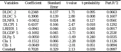
There are two equations in the form two-error corrections terms and contain restricted long-run stationary relationship. Taking both lagged one period as explanatory variables in the system; we can produce the short-term dynamics, which consists of six equations of changes in LDC, LNFA, LFg, LREER, LGDP and LCPI. The results for the whole equations are presented at Annex IV. However, our interest is to know the Monetary Authority of Ethiopia reacts to macroeconomic shocks using domestic credit as monetary policy variable so that we present the equation of LDC reported in Table 8. The VECM is estimated as presented by (Badawi, 2005; Doornik and Hendry 2001). On top of this, it is better to follow general-to-specific modeling specification by deleting statistically insignificant explanatory variables to obtain a parsimonious model (leaving from over parameterized equation) and check the validity of the model through tests. This is mainly attributed to the fact that the probability of having a statistically

insignificant coefficient for all variables (small t value), the lack of meaningful relation, and the inexistence constancy of parameter or taking variable as exogenous in the system where

it is endogenous (Doornik and Hendry, 2001). Therefore let’s set the lag length at eight (over parameterized equation) and follow the general–to-specific procedure to the most parsimonious dynamic LDC equation considering t-value and other criteria. Finally, it yields the following parsimonious short run dynamics of monetary variable, LDC in Table 8. In the short run dynamics equation, real effective exchange rate, and consumer price index are statistically significant at lag one. On top of this, both domestic credit and GDP are statistically significant at lag five. However, only DLDC-5 and DLCPI-1 have a positive short-term effect on domestic credit while others placed on negative effect. Moreover, both error correction terms are statistically significant with negative short-term effect on DC. It means that the coefficient is CIa-1 and CIb-1 indicates the speed of adjustment towards the long run equilibrium or relation for equation LDC and DLNFA respectively.

Table 8. Parsimonious Dynamic LDC equation

Variables Coefficient Standard

Error

t-value t-probability Part.R^2

DLDC_2 0.2348 0.137 1.71 0.095 0.0663

DLDC_5 0.3908 0.139 2.80 0.008 0.1607

DLNFA_1 -0.0452 0.024 -1.86 0.127 0.0560

DLCPI_1 0.4107 0.166 2.47 0.018 0.1292

LREER_1 -0.0941 0.046 -2.03 0.048 0.0917

DLGDP_5 -0.1692 0.045 -3.73 0.001 0.2538

DLFg_5 -0.0050 0.003 -1.69 0.240 0.0335

CIa_1 -0.1512 0.066 -2.28 0.028 0.1126

CIb_1 -0.0649 0.032 -2.01 0.051 0.0894

Constant 0.7028 0.329 2.13 0.039 0.0997

Source: - Estimation of Short Run Dynamics for LDC

Sigma = 0.0342166, RSS=0.048001793, R^2=0.428059, Log-likelihood: 107.897, -T/2log|Omega| 181.681776, No. Of observations: 52, no. Of parameters=11, Mean (DLDC) 0.02777, Var (DLDC)= 0.001614, Sigma = 0.0342166, DW = 1.88

Diagnostic Tests:

AR 1-4 test: F (4,37) = 0.35190 [0.8410] ARCH 1-4 test: F (4,33) = 0.71613 [0.5869] Normality test: Chi^2(2) = 0.16248 [0.9220] Hetero test: F (20,20) = 0.79611 [0.6925] RESET test: F (1,40) = 2.1383 [0.1515]

In the equation of DLDC, the coefficient of DLNFA is equal negative 0.0452, while in equation of DLNFA the coefficient of DLDC is 0.27 and 0.48 at lag-1 and lag-5 (see Annex IV that states the single equation of LNFA up on general to specific procedure). The coefficient’s sign for DLCPI-1 is Table 7. Restricted standardized adjustment coefficient 

Adjustment coefficient LDC LNFA LCPI LREER LDGP LFg

1 0.02072 0.45895 0.15795 -1.1043 -0.33726 0.00000

(1.78) (1.65) (2.95) (-3.92) (-3.02) (Res)

2  0.01714 0.11133 0.13353 -0.16206 -0.15205 0.0000

(-1.93) (1.61) (-3.57) (-3.35) (-2.79) (Res)

Source: - Estimation Results of Restricted standardized adjustment coefficient 

positive while DLNFA-1, DLREER-1 and DLGDP-5 reported with a negative sign. DLFg is statistically insignificant to explain the variation in LDC. Moreover ECM reported with correct sign and statistically significant. Finally, regarding to diagnostic tests, there is no autocorrelation and heteroscadicity problem among residuals. On top this, the normality condition is satisfied and RESET test also depicted that there is no model specification problem in the system. (Note that variables at specified lags are included in the model to maintain the best of diagnostic tests as reported and very important for evaluation of monetary policy objectives against theory).

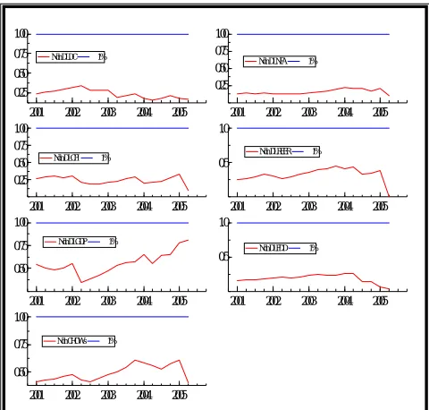
Stability tests

The intuition behind stability test is to check the monetary policy reaction function stability and predictability for policy analysis in responding to macroeconomic shocks. To test the stability of parameter, the study conducted the recursive least square graphic test which can overcome the limitation of the chow test (it does not indicate the source of instability, whether from the intercept or the coefficient upon dividing the sample into two groups). The recursive method uses by increasing the sub-sample size and then estimate the parameters continuous until the total sample data is completed. So finally plot the paths of the estimates over time. In recursive plots, there are two standard error band around the selected coefficients. As the sample size increase and significant variation occur within the bands, then the coefficient is stable over the entire period and indicates the constancy of the variance of the estimated model. Therefore up on this theory, the recursive graphs that plot 1-step- ahead residuals, break point chow tests and 1-1-step-ahead chow-test for the LDC and other variables in the system reported graphically below.

Source: - Estimation Results for stability test using recursive least square graphic test

Figure 1. Constancy Parameter statistics: 1-step-ahead residuals

Hence the graphs presented in the Figure 2 suggest that the model is stable and can be used for prediction of monetary policy reaction function. When you mark the 1-step-ahead residuals entries in the PC-GIVE dialog window, the 1-errors

lies within their approximate 95%confidence bands with constant standard errors reported that the time path of estimates plotted within error band justify the stability of model and accept constancy of the parameters. When we mark the break point chow tests with a 1% significance level, we have the following graphs indicate that there is no break-point chow test anywhere significant given the 1% line plotted on top of each of the graphs. The last plot is the overall system constancy test that justifies the model is stable.

Source: - Estimation Results for stability test using Break point chow tests

Figure 2. Constancy Parameter statistics: Break point chow tests

Granger Causality Tests for NFA and DC

Noting that broad money supply basically consists of net foreign assets and domestic assets, and we know that the Monetary Authority of Ethiopia needs to equalize the growth rate of the money supply at the growth rate of GDP with a strong macroeconomic surveillance. In addition, the monetary approach to the balance of payment states that the movement of net foreign assets (NFA) can be influenced by the domestic credit (DC) expansion. Their relation extended to determine the internal and external imbalance of the economy, but some studies gave reasons for reverse causality between NFA and DC. During a decrease in NFA before DC is cut, the crowding out effect of the government credit cut DC and secondly the decrease in NFA leads to lower the reserve base (the summation of currency in circulation and Bank deposit in Central Bank), which has effected on commercial banks’ lending. But their lending is not as such responsive to reserve base due to the already existing excess reserve above the requirement in the case of Ethiopia. Following both variables are assumed to be stationary at first difference level and the errors terms entering the causality test are uncorrelated, the Granger causality test of net foreign assets and domestic credit based on quarterly periods of 1991-2005 can be presented below in the Table 9.

2001 2002 2003 2004 2005

-0.05 0.00 0.05

r DLDC

2001 2002 2003 2004 2005

-0.25 0.00 0.25 0.50

r DLNFA

2001 2002 2003 2004 2005

-0.05 0.00 0.05

r DLCPI

2001 2002 2003 2004 2005

-0.1 0.0 0.1

r DLREER

2001 2002 2003 2004 2005

-0.2 0.0 0.2

r DLGDP

2001 2002 2003 2004 2005

-1 0 1 2

r DLFDD

2001 2002 2003 2004 2005 0.25

0.50 0.75 1.00

Ndn DLDC 1%

2001 2002 2003 2004 2005 0.25

0.50 0.75 1.00

Ndn DLNFA 1%

2001 2002 2003 2004 2005 0.25

0.50 0.75 1.00

Ndn DLCPI 1%

2001 2002 2003 2004 2005 0.5

1.0

Ndn DLREER 1%

2001 2002 2003 2004 2005 0.50

0.75 1.00

Ndn DLGDP 1%

2001 2002 2003 2004 2005 0.5

1.0

Ndn DLFDD 1%

2001 2002 2003 2004 2005 0.50

0.75 1.00

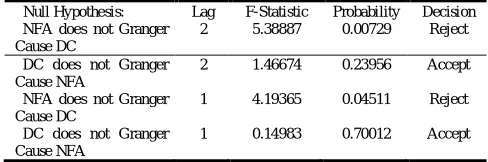
Table 9. Granger causality test

Null Hypothesis: Lag F-Statistic Probability Decision

NFA does not Granger Cause DC

2 5.38887 0.00729 Reject

DC does not Granger Cause NFA

2 1.46674 0.23956 Accept

NFA does not Granger Cause DC

1 4.19365 0.04511 Reject

DC does not Granger Cause NFA

1 0.14983 0.70012 Accept

Source: - Estimation for Granger causality

As noted above, at lag length one and two, only unilateral feedback effect direction from net foreign assets to domestic credit. It implies that the Monetary Authority of Ethiopia can control the availability domestic credit to react macroeconomic shocks. In other word, any shocks in net foreign assets cause change in domestic credit, consistent with our model.

Interpretation of the Results

Up on the estimates presented above, we can now interpret both long run and short run dynamic analysis. This empirical discussion focuses on the response of the Monetary Authority of Ethiopia to macroeconomic shocks. Let us have a look at the long run dynamics model. Since the exogeneity nature of fiscal gap (LFg), domestic credit has positive long run effect to net foreign assets and gross domestic product while it has very low elasticity to the real effective exchange. This implies that the Authority took action using domestic credit on the basis of net foreign assets, as both are the determinants of money supply. Both are required to respond at the same growth rate of GDP. However, the RRER that measures the international position of the country in competition of the country has an insignificant impact on domestic credit that held by the Authority. This is because of backward technology, poor quality products, structural problem, macroeconomic imbalance, political instability and the like. Regarding to the consumer price index, the policy variable had small elasticity to the change in the CPI in the long run, which implies that inflation happened not only from the monetary effect, but also from aggregate supply shortage evidenced by a positive correlation between drought and war with inflation over the period 1991 to 2005. Due to the consequence of the coffee export booming and the substantial increment in credit expansion in the private sector, there was a significant change in the growth of GDP during 1994/95 and followed lower inflation. It continues with fluctuations due to the EL Nino weather condition, and Ethio-Eritrea conflicts during 1997/98 and the drought occurred all over the country in 2001/02 negatively affect the growth rate GDP and brought higher upward change in the consumer price index (NBE, 1998). Regarding to fiscal gap, domestic credit has the positive long run effect to fiscal gap if we take the fiscal deficit as an endogenous variable (but became weak effect when we treat it as an exogenous variable for the system). This is also directly consistent with theories in the case of developing countries. In the absence of broad and active financial market the primary obligation of monetary authorities is to finance the government deficit. Under such circumstance monetary growth primarily depends on fiscal policy (Joyce, 1991).

Even though the Monetary Authority does not have full control over it, net foreign assets have positive long run relation with LCPI and trend while it has the negative relation with LREER, LGDP and LFg (similar output done by Haile Kibret, 2001 in the study of BOP and policy). On top of this, all explanatory variables are statistically significant and LNFA has strong relation with them: that is why Monetary Authority articulates policies using domestic credit along with the position of net foreign assets as both are the determinants of money supply and used to set the rate equal to the annual growth rate of GDP growth rate in Ethiopia. Restricted standardized adjustment coefficient, 1=0.02072 tells us that the speed of adjustment or

feedback effects towards the long run equilibrium is 2.072 percent per quarter when there is a macroeconomic shock to the system, which is very weak took 8.288 percent per annum. In general, it took many years for full adjustment. This is a rationale for the length lags structure and undeveloped financial sectors that slow down the effectiveness of monetary policies, and disable its ability to govern macroeconomic shocks within a short period. It is obviously noted that one of the efficiency measurement criteria for monetary policy is the time taken for adjustment and the controllability of macro variables.

Bearing the long run dynamic analysis in mind, we can interpret the short run empirical outcomes for policy prescription from table 8. Both domestic credit at lag 5 and GDP at lag 1positivly influence the monetary policy of domestic credit and are statistically significant. This indicates that monetary policy variable, DLDC, has a dynamic nature and can be affected by lag structure. However DLNFA is a loose significant and negative short run impact indicating that variations in LDC are not much more explained by a change in LNFA in short run period, and also DLFg could not explain the change in DLDC. Both error correction terms are statistically significant with negative short-term impacts on DLDC, which is consistent with the two Co integrating vectors. It means that the coefficient is CIa-1 and CIb-1 indicate the speed and direction to correct equilibrium errors towards the long run relation are 15.12% and 6.49% per quarter where there is a shock in the short run dynamics, implying that inconsistent with the long run dynamic analysis. In the equation of DLDC, the coefficient of DLNFA is known as sterilization coefficient, which measures how much change in the net foreign assets deriving from the interventions in the exchange rate market is sterilized by the monetary authority. In general, it is an indicator of the degree of sterilization of net foreign assets. The coefficient ranges from zero to minus one. If it is a negative one, the sterilization is complete; while it is greater than one, the degree of sterilization is less than full (Olcay and Almila, 2000). Therefore, from table 8, the coefficient of –0.0452 tells us incomplete sterilization activities done by the Monetary Authority of Ethiopia. In equation of DLNFA (see annex IV) the coefficient of DLDC is known as the offset coefficient, which gives the amount of capital outflow per domestic currency of expansion of domestic credit. It closes to –1 if domestic and foreign assets are close substitutes indicating a higher degree of capital mobility and a low degree of control over the money stock. If it closes to zero, a higher degree of monetary control and a low degree of capital mobility are available (Olcay and Almila K, 2000). Accordingly the

coefficient of model under investigation 0.29 and 0.48 at lag-2 and lag-5 are closer to zero even though its t-value is statistically insignificant. Therefore the Monetary Authority of Ethiopia adopted a higher degree of monetary control with a low degree of capital mobility in practices. Comparing the result against the theories, the coefficients’ signs for DLNFA-1 and DLCPI-1 indicate that Authority follows accommodating monetary policy while DLREER-1, DLGDP-5 and DLFDD-5 reported like where there is strict stabilization monetary policy

is exercised. In summary, the Authority conducted a mixed pattern of coefficient value indicating a combination of both policies was followed.

Conclusion and Policy Implication

Since the onset of market oriented economy in 1991, the government introduced series economic reforms in the context of structural adjustment program of the World Bank and liberalization program of the IMF. These include improving external imbalance, liberalizing trade and financial sectors, and to remove fiscal and real sector constraints. In this regard, the Monetary Authority of Ethiopia has been playing a prime role in stabilizing the macroeconomic system, particularly maintaining price stability and achieving international targets. This is conducted via indirect monetary policy instruments like removing discriminatory and ceiling restriction on interest rates among sectors, Treasury bill market as a stepping-stone for open market operations. Moreover, the monetary policy has been shifted towards the objective of reducing monetization of budget deficits in order to lower inflation in the reference period, 1991-2005.

In doing so, the Monetary Authority of Ethiopia has reacted to the existed macroeconomic shocks in line with making the broad money supply growth rate at the rate of nominal GDP. For keeping a proper response and monetary policy objective, the Authority has considered monetary growth rate as determined by domestic credit and net foreign assets from which domestic credit is chosen as a policy variable while monetization of fiscal deficits, consumer price index, economic growth, net foreign assets and real effective exchange rate are taken as determinants of monetary policy. The Authority then adjusted its operating and instruments targets to new information mostly using quarterly and annual frequency in the sense that to create a link between short term and longer horizon monetary objectives. The monetary policy of domestic credit, therefore, has strong long run and positive relation with net foreign assets and real GDP in the long run. However, it has short-run relation to the change in domestic credit and real GDP at lag five, and with the change in both CPI and REER at lag-one. The equilibrating error terms derived from both LDC and LNFA in the long run have strong negative relation with LDC in the short run. Eventually, the result justifies that the Authority follows a combination of accommodating and stabilizing policies in the review period. In summary, the Authority has strongly met the objectives of reducing the monetization of budget deficits and the effort of setting the monetary growth rate of the growth rate of nominal GDP over the period 1991- to 2005. In addition, the objective of stabilizing the price level is determined not by the monetary phenomena. Rather, it was directly linked with the agricultural

supply bottlenecks like erratic rainfall, drought, political instability and war. The longer speed of adjustment manifested the poor effectiveness as evidenced by the efficiency measurement criteria for monetary policy.

The policy implication of the empirical result tells us that the net foreign assets (international reserves), inflation, real effective exchange rate and real GDP should be considered in conducting and analyzing monetary policy. Accordingly, the Authority should also pay attention to part of the broad money determinants, net foreign assets to respond macroeconomic shocks, and more emphasis should be continued to the objective of price stability and achieving international reserve target. In addition the effort to reduce deficit monetization has been successfully satisfied in the short and long run in the review period to control inflationary condition. The low long run adjustment coefficient indicates the inadequacy of the financial market and weak financial development, which in turn implies that the indirect monetary policy instruments might not be effective as expected. Therefore the following policy implications are suggested. The effectiveness of monetary policy, including the controllability of the Authority over macro variables depends on the demand pattern of the economy, which is activated by performance of investment. Thus, the government should conduct policies that improve structural bottleneck in the real sectors. These enable the commercial banks to extend credit (short term and long term) to private sectors and minimize their over-liquid cash position, manages the money supply using the interest rate. Therefore, the Authority has to make investigation and pursue policies that enable commercial banks to utilize their over-liquid assets. The Authority has to continue to pursue policies of reducing budget deficits monetization to control inflation rate even though the government has already shifted to pro-poor macroeconomic policies and sustainable development programs. On top of this, as we have seen in restricted long-run model, the domestic credit does not have significant elasticity and relation to the consumer price index in the long run indicating that the Authority controlled inflation only to some extent due to the non-monetary nature. Therefore, the government should pay attention for policies that improve aggregate supply hence export bottleneck. Even though the developing Treasury bill market was taken to lay ground for open market operation, it was delayed to move out to a fully fledged open market even at the end of fifteen years after liberalization. Hence, the Bank has to make the transition period shorter by establishing economically and institutionally strong financial and privates sectors.

REFERENCES

Adam, S. 1976. "An Inquiry into the Nature and Causes of the Wealth of Nations", Kathryn Sutherland (Editor), 2008, Oxford Paperbacks, Oxford, ISBN 978-0-19-953592-7.

Annex I:-Stationary Test Using Graphic Presentation

Badawi, A. 2005. "Testing Stationary in Selected Macroeconomic Series in Sudan”, Journal of African Economies, University of oxford.

Chang 2000."Monetary policy Reaction Function for Selected Developing Countries”, International Journal of applied economics, March 2000,PP 50-61.

Clarida, R., Gali, J. and Gertler, M. 2000. "Monetary Policy Rules and Macroeconomic Stability: Evidence and Some Theory”, The Quarterly Journal of Economics, 115(1),147-80.

Danial and Van Hoose 2002. "Monetary Approach to Balance of Payment and Exchange rate determination".

Doornik and Hendry, 2001. "An Interface to Empirical Modelling", 2ND Edition, UK.

Einar, R. 2000. "Macroeconomic stability as a precondition", Bank of Latvia.

Enders 1995. "Applied Econometrics in Time Series” New York.

Equare D. 1994. "Exchange Rate Instability and its consequences”, Central Bank of Ethiopia, Quarterly bulletin Birritu No.56.

Fisher, J.D.M. 2006. "The Dynamic Effects of Neutral and Investment-Specific Technology Shocks”, Journal of Political Economy, 114(3), 413–451.

Friedman, M. 1968. "The Role of Monetary Policy", The American economy review, Vol.58

Friedman, M. 1970. "A Theoretical Framework for Monetary Analysis”, Journal of Political Economy.

Gazena, E. 2001. "Monetary Policy instrument in Ethiopia", NBE Quarterly Bulletin Birritu No. 78.

Goldstein, M. and Khan, M.S. 1976. "Large Versus Small Price Changes in the Demand for Imports", IMF Staff Papers, 23, 200-225.

Haile, K. 2001. "Monetary Policy and Balance of Payment in Ethiopia", Central Bank of Ethiopia, Addis Ababa, Ethiopia.

Hallowed and MacDonald 1989. "International Finance Economy".

Harris, R. 1995. "Using Co-integration Analysis in Econometric Modeling", London.

Johansen, S. 1995. "Likelihood-Based inference in co-integrated vector model", Oxford University.

John, M. 2004."The Philippine central Bank’s monetary policy Reaction function", University of Philippine.

John, W. and Shruti, P. 2007. "Economic Policies, MDGs, and poverty: Fiscal Policy, Center for Development", Policy and Research Paper, School of Oriental and African Studies.

Jose, A. 2002. "Macroeconomic Stability in Developing countries", NACLONES.

Joyce, J. 1991. "Examination of Monetary Policy objectives in Four Different Countries", World Development economics Journal Vol.25, PP16-37.

Justiniano, Alejandro, and Giorgio 2008. "The Time-Varying Volatility of Macroeconomic Fluctuations", American Economic Review, 98(3):604-41.

Keynes, J. M 1936. "The General theory of employment, interest and Money", London, Macmillian.

MOFED 1999. "Survey of the Ethiopian Economy, for the period 1992/93-197/98 related issues on Macroeconomic performance of Ethiopian Economy", Addis Ababa. NBE 1995, 1998, 2004. "National Bank Annual and Quarterly

Report various issues", Ethiopia.

Olcay and Almila 2000. "Monetary Policy Reaction Function In Turkey”, Central Bank of Turkey.

Phillips, P. 1987. "Time Series Regression with a Unit Root", Econometrica, 55,227-301.

Said S., and Dickey, D.A. 1984. "Testing for Unit Roots in Autoregressive-Moving Average Models of Unknown Order", Biometrika, 71,599-607.

Sylvanus I. 2004."Issues in Stabilization policy Options", AERC Kenya Nairobi.

Thomas, H. and John, T. 1980. "Current Issues in Monetary Theory and Policy", Duke University.

Vijay, 2003. "Exchange Rate Regimes: Is there a third way?", Research School of Pacific Studies, Australian National University.

Yimeserach 2005. "The Behavior of Money supply in Ethiopia", Addis Ababa University

Annex I:-Stationary Test Using Graphic Presentation

Annex II: -Decomposition of Aggregate GDP into Quarterly GDP

This is directly taken from the research paper undertaken by Haile Kibret-NBE-entitled “BOP and monetary policy”. Ethiopian GDP is highly affected by seasonality of agricultural harvest. This is mainly due to the fact that agriculture is rain fed. The structure of agriculture harvest is divided in to main harvest, which account about 95% of the total agriculture GDP, and the Belg harvest that accounts for the balance. According to information obtained from CSA, anything harvested between September and January is classified as main harvest; And the rest are Belg harvested. Moreover, a survey by CSA has also suggested that about 80 % of agricultural GDP are cereals.

1990 1995 2000 2005

9.5 10.0 10.5 LDC

1990 1995 2000 2005

-0.05 0.00 0.05 0.10

DLDC

1990 1995 2000 2005

5.0 7.5

10.0 LNFA

1990 1995 2000 2005

0 1

DLNFA

1990 1995 2000 2005

4.25 4.50 4.75

5.00 LCPI

1990 1995 2000 2005

0.0 0.1

DLCPI

1990 1995 2000 2005

4.5 5.0

5.5 LR EE R

1990 1995 2000 2005

-0.1 0.0 0.1 0.2

D L RE R

1990 1995 2000 2005

8.0 8.5

LG DP

1990 1995 2000 2005

0.00 0.25 0.50

D L GD P

1990 1995 2000 2005

4 6 8

LFD D

1990 1995 2000 2005

-2.5 0.0

2.5 D L FD D

Studying the behavior of quarterly contribution of the agricultural sector to the total GDP is computed based on the amount of labour exerted to each activity in the production of cereals for which date is available. The data and the computed coefficients are presented below:

The allocation of each economy to each activities and the derivation of the coefficients are performed as follows. These coefficients give the quarterly weight of agriculture output. July, August and Sep (Q1) = Sowing and first weeding; Oct, Nov, Dec (Q2) = 2nd weeding and harvesting; Jan, Feb, Mar (Q3) = threshing; April, May, Jun (Q4) = plough(1st, 2nd, 3rd).

For each quarter the coefficient are: Q1 = 0.075 +0.268 = 0.343,

Q2 = 0.089 + 0.194 = 0.283, Q3 = 0.179, Q4 = 0.075 + 0.075 +

0.045 = 0.195. Since the Belg season (small rain season) is very small, about 5% relative to the main season, it is ignored.

Regarding to services Sectors (as represented by the distribution sub- sector), the quarterly seasonal adjustment coefficients are calculated for the distributive sub-service sector based on loan disbursement from the banking system. The distributive sub-sector includes trade, hotels and restaurants and transportation and communication. The distributive sub-sectors accounts for about 75 % of the total service sector’s GDP. It is also believed that the distributive sub-service sectors activity uses bank credit in the form of overdraft facility and term loans, the time series quarterly disbursement of bank loan to the distributive service sector is available from NBE bulletin and data. For other service, however, the annual data is equally divided in to the 4th quarter because this sub- sector is beloved to be less seasonal sensitivity. The average quarterly disbursed as well as the corresponding ratios are provided in the following Table:

Regarding to industrial Sector, the coefficient for seasonality of industry in the total GDP are computed from quarterly production data compiled by Ministry of Economics and Development on twenty eight manufacturing public enterprises which data is available since 1993. The coefficients are:

Total Ratio

Q1 1162178 0.217

Q2 1385103 0.259

Q3 1412160 0.265

Q4 1388841 0.259

Total 5348282 1.00

After getting the coefficient of agriculture, industry and service sector, for each Q, we multiply the annual GDP by each coefficient to get quarterly sectoral value and then add them to generate the quarterly annual GDP.

Annex III: -How NBE generates Real Effective Exchange Rate

REER is the measure of the price of the country’s goods to the price of its trading partner countries, both expressed in domestic currency. The index is calculated by taking quarterly data on wholesale price index, which is used as a proxy for the world price of tradable while the consumer price index of the home country was used as a proxy for the domestic price of non-tradable. For such construction, the performance in 1995 is taken as base year, which seems normal in that there was no war and drought in the country. Individually, trading partner countries were selected by employing a one percent threshold in which countries having a trade share of more than 1% for inclusion in the construction of REER. Jointly countries have a share of 80% in total trade of Ethiopia. Hence all variables are computed and organized from the quarterly Bulletin of NBE. Note that an increase in REER index indicates appreciation. REER is the index is computed by taking quarterly data on wholesale price index and exchange rate of 19 major trading partners (Belgium, Kenya, Italy, France, Germany, Us, Uk, S.Arabia, nether land, south Korea, Sweden, Japan, India. are selected by their weight of import plus expire to total hade of Eth and accounted 80% of total trade jointly) and applying weighted trade index to the base year of 1995 which seem to be normal in that there was no war/ drought in the country. NEER stands for Nominal Effective Exchange Rate and REER stands for Real Effective Exchange Rate

Labour requirement for different activities for selected cereals (in man-days)

Barely Wheat Teff Maize Sorghum Average Cash

1st

plough 4 4 5 7 5 5 0.075

2nd

plough 4 4 5 7 5 5 0.075

3rd plough 3 3 5 3 - 3 0.045

Planting, sowing covering 4 4 6 8 4 5 0.075

1st

weeding 15 11 22 20 24 18 0.268

2nd

weeding - - - 24 7 6 0.089

Harvesting 13 18 18 9 9 13 0.194

Threshing, Widowing (shelling) 7 10 17 19 9 12 0.179

Total 50 54 78 88 63 67 1.00

Source: - CSA, Development Bank of Ethiopia, and Ministry of Agriculture

Average Quarterly disbursement for distribution service and computed coefficients

Distribution Service Quarter1 Ratio Quarter2 Ratio Quarter3 Ratio Quarter4 Ratio

Domestic Trade 458 0.164 3351.5 0.377 2705.3 0.304 1368.6 0.154

International trade 791.4 0.184 1006.4 0.234 1476.2 0.344 1019.8 0.237

Hotels and Restaurants 300.2 0.258 314.7 0.271 247.4 0.212 299.8 0.257

Transportation and Comm. 459.1 0.198 598.6 0.258 566.4 0.244 693.1 0.299

Average Ratio 0.201 0.285 0.276 0.237

Other service 0.25 0.25 0.25 0.25

Source: Various issue of NBE