Prediction of Concrete Faced Rock Fill Dams Settlements
Using Genetic Programming Algorithm
Seyed Morteza Marandi, Seyed Mahmood VaeziNejad, Elyas Khavari Civil Engineering Department, Shahid Bahonar University, Kerman, Iran
Email: [email protected], [email protected]
Received January 16, 2012; revised March 30, 2012; accepted April 7, 2012
ABSTRACT
In the present study a Genetic Programing model (GP) proposed for the prediction of relative crest settlement of con- crete faced rock fill dams. To this end information of 30 large dams constructed in seven countries across the world is gathered with their reported settlements. The results showed that the GP model is able to estimate the dam settlement properly based on four properties, void ratio of dam’s body (e), height (H), vertical deformation modulus (Ev) and shape factor (Sc) of the dam. For verification of the model applicability, obtained results compared with other research meth- ods such as Clements’ formula and the finite element model. The comparison showed that in all cases the GP model led to be more accurate than those of performed in literature. Also a proper compatibility between the GP model and the finite element model was perceived.
Keywords: Concrete Faced Rock-Fill Dams; Settlement; Genetic Programming Algorithm; Finite Element Model
1. Introduction
One of the most important reasons of dam failures is un- controlled settlements. Especially in the case of earth dams due to weak compaction and the use of improper materials this may occur. Such phenomenon may lead to very huge economic costs and human casualties but it has not been studied completely yet.
In the last centuries various concrete faced rock-fill dams are designed and constructed in many countries across the world. Exclusively in the past decades, the de- signing process and their construction has been changed considerably [1]. Such phenomenon occurred specially for the concrete faced rock fill dams. Recent growing demands for taller and larger dams, has changed the fun- damental rules dominant in their design. This has led to new theories on the basis of new methods of testing ma- terials and new techniques for the analysis.
Basically deformation of a dam may happen in three steps or situations: during the construction, during the first impounding, and while servicing. There are two basic approaches found in the literature for the estimation of the crest and body settlement in dams: 1) Numerical methods such as the finite element method, finite differ- ence method; and 2) Experimental methods.
Almost all methods exist for prediction of dam de- formations cover only one or two steps of the three steps mentioned above. For example, finite element method is used for the analysis of dam deformation during
con-struction and first impounding. While, experimental me- thods are used for estimation of dam deformation during construction and servicing [2].
Sowers et al. in 1965 gathered information of 14 dams without attention to their heights, methods used in their section design, material used in the dam body and their construction methods and draw a scatter chart for height of dams over logarithm of the time. While better methods of construction e.g. better compaction or better proofing de- crease the amount of settlement, they indicated that the settlement is independent of all these factors [3].
Lawton and Lester (1964) used data of 11 dams where, their settlement were at least 0.02 percent of their heights and presented in a settlement equation. The equation used depends only on the height and is not related to the time needed for the settlement [4].
Soydemir and Kjaemsli (1979) combined displacement equations in respect to time and height and obtained a new equation for the displacement of dam in various time periods using 48 different dam settlements data [5].
ments [6].
Pinto and Marques Filho in 1998 presented a simple way for an approximate estimation of concrete faced rock-fill dams (CFRD) deformations. Their investiga- tion showed that the void ratio and downstream valley shape have the most important effect on the deformation modulus1 of under construction dams. Accordingly for narrow valleys whose shape factors are less than 3.5, the effect of valley shape is higher than those with bigger shape factors2 (SF > 4). This means in wider hills the void ratio is more effective [8]. They also presented the following equation for the vertical deformation modulus.
1000 h
S v
E H
b S aH
(1)
where Ev is vertical deformation modulus, H is embank- ment height above a determined point in meters, h is embankment height below a determined point, γ is em- bankment density in KN/m3 and s is the settlement of specified point in meter [9].
The Finite element method is a new method in com- parison with the other methods used in the literature. Its reliability is highly dependent on the selected constitutive model for materials and an appropriate meshing which best cover the real environment. Kovacevic (1994), Dun- can (1992, 1996) are the first investigators who used the finite element methods for the study of rock-fill em- bankment deformations during dam construction and the first impounding. They discussed on the analysis meth-ods, limitations and combining different stress-strain models and their errors. Based on Duncan’s studies, a good correlation exists between the estimated and ob-served values [10-12].
Frequently, the estimation of dam properties is based on the experiments of previously constructed dams. There is much information published for estimation of concrete faced rock-fill dams. However these papers are written on the basis of limited information and in almost all cases concentrated on one or two of the effective pa-rameters on rock modulus of elasticity or measured de-formation. To overcome these limitations and present a simpler method, genetic programming algorithm which is of interest of various engineering fields can be aproposed method for the prediction of dam crests deformations. Due to high complexity and the presence of different variables in the soil responses, the genetic programming with a perfect training algorithm is extended. However, the authors could not find any data obtained for
estima-tion of crest settlement of concrete faced rock-fill dams using GP algorithm in literature. In this paper an investi-gation is carried out on the deformation behavior of con-crete faced rock-fill dams using GP modeling. For this purpose, documents from 30 information bases and from 7 countries across the world are used. The studies are concentrated on four effective parameters for prediction of dam crest settlement. These parameters are: void ratio of dam’s body (e), height of dam (H), vertical deforma-tion modulus (Ev) and shape factor of the dam (SF). For training of the model, 67 percent of information (infor-mation of 21 dams out of 30 dams) is randomly selected and 33 percent of the rest (information of 9 dams) is used for dam prediction testing. To verify the suggested model with other methods in literature, the prediction results obtained for concrete faced rock-fill dams is compared with the Clement method.
2. Behavior Characteristics of Concrete
Faced Rock-Fill Dams (CFRDs)
Due to the better performance and lower costs, construc- tion of the concrete faced rock-fill dams (CFRDs) have been used wide spread since 4 decades ago. The CFRDs have become more common than rock-fill dams with clayey cores. Experience showed that even though these types of dams are economical and reliable, but in most cases the concrete decks are exposed to failure, damage and settlement. Table 1 shows performance and struc- tural properties of CFRDs used in the present study [13].
Clements studied on the real settlements of 68 earth dams after construction and compared the results with the estimated values derived from the following equa- tion:
(2) where S is the crest settlement in meters, H is the height of dam in meters, a and b are experimental constants of the equation. The constants values are given in Table 2.
Table 3 shows the measured values of the crest set- tlements of 35 dams in the fields and estimated values using Clements experimental equation for period of 10 years after construction. Statistical analysis between these two type of data shows that there is a weak correla- tion of R2 = 0.201 between the results. Therefore, it seems the Clements method is very conservative.
3. The Genetic Programing (GP) Model
3.1. Structure of the GP SDEL
1For determining deformation behavior of rocks, deformation modulus
during construction (Erc) and during the first filling (Erf) are defined
which are related to its void ratio and the bed rock properties. Theo-retically vertical deformation modulus (Ev) gradually decreases with
increase in the dam’s height [7].
2SF = A/H2 where H is embankment height in meters and Ais the area
of upstream deck area in squared meters.
Table 1. Performance and structural properties of CRFDs [13].
After impounding No. Dam Country Year Height(m) Shape factor (A/H2) Void ratio (MPa)EV
Time (year) Crest set. (m) Crest set. (%)
1 Cethana Australia 1971 110 2.5 0.26 140 30 0.176 0.160
2 Alto Anchicaya Colombia 1974 140 1.1 0.22 145 10 0.173 0.124
3 Golillas Colombia 1978 127 0.9 0.24 155 7 0.057 0.045
4 Sugaroaf Australia 1979 85 11.5 0.302 55 16.2 0.207 0.244
5 Foz do Areia Brazil 1980 160 5.4 0.33 47 20 0.210 0.131
6 Mackintosh Australia 1981 75 4.9 0.24 45 19 0.235 0.313
7 Mangrove creek Australia 1981 80 4.5 0.26 75 4 0.084 0.105
8 Tullabardine Australia 1982 26 8.1 0.23 90 12.8 0.019 0.076
9 Murchison Australia 1982 94 1.9 0.234 190 18 0.082 0.087
10 Bastyan Australia 1983 75 3.4 0.23 160 9 0.053 0.071
11 Salvajina Colombia 1983 154 2.4 0.21 205 7.5 0.090 0.061
12 KhaoLaem Thailand 1984 113 11 0.29 59 14 0.187 0.165
13 Shiroro Nigeria 1984 125 4.2 0.2 76 1.8 0.166 0.133
14 Kotmale Sri Langka 1984 90 7.4 0.27 50 - 0.150 0.167
15 Dongbok Korea 1985 44.7 3.5 0.27 26 7 0.043 0.096
16 Lower Pieman Australia 1986 122 2.5 0.24 160 15 0.221 0.181
17 Pyonghwa (1st) Korea 1988 80 7.1 0.4 71 5 1.168 1.460
18 Chengbing China 1989 74.6 2.8 0.277 100 10 0.100 0.130
19 White Spur Australia 1989 43 2.3 0.215 180 5.9 0.058 0.135
20 Xibeikou China 1989 95 3.3 0.284 80 6 0.061 0.064
21 Crotty Australia 1990 83 1.9 0.20 375 9 0.056 0.067
22 Segredo Brazil 1993 145 4.1 0.37 45 8 0.229 0.158
23 Aguamilpa Mexico 1993 187 3.9 0.18 190 7 0.340 0.182
24 Xingo Brazil 1994 150 6.0 0.28 34 6 0.931 0.621
25 Wananxi China 1995 93.8 2.0 0.257 100 - 0.336 0.358
26 Buan Korea 1996 50 7.3 0.25 25 11 0.204 0.408
27 Tianshenqiao China 2000 178 4.9 0.31 45 1.5 1.060 0.596
28 Ita Brazil 2000 125 7.0 0.308 48 3 0.600 0.480
29 Yongdam Korea 2001 70 8.8 0.32 52 6 0.123 0.176
30 Miryang Korea 2001 89 6.8 0.18 90 6 0.088 0.099
31 Namgang Korea 2001 34 36.2 0.27 47 6 0.013 0.038
32 Sancheong (L) Korea 2002 70.9 6.3 0.27 83 6 0.087 0.122
33 Sancheong (U) Korea 2002 86.9 3.1 0.27 92 6 0.300 0.345
34 Jangheung Korea 2005 53 10.7 0.28 34 1 0.015 0.028
35 Daegok Korea 2005 52 3.7 0.25 154 1 0.019 0.037
Table 2. Constants values of a and b [6].
Constants Initial impounding After 10 years
a 0.0002 14 × 10−7
[image:4.595.58.282.187.732.2]b 1.1 2.6
Table 3. Comparison of measured and estimated settle- ments values [13].
No. Dam crest set. (m)Measured Estimated Crest set. Clements theory (10 years service)
1 Cethana 0.176 0.284
2 Alto Anchicaya 0.173 0.532
3 Golillas 0.057 0.413
4 Sugaroaf 0.207 0.145
5 Foz do Areia 0.210 0.753
6 Mackintosh 0.235 0.105
7 Tullabardine 0.019 0.007
8 Murchison 0.082 0.189
9 Bastyan 0.053 0.105
10 Salvajina 0.09 0.682
11 KhaoLaem 0.187 0.305
12 Shiroro 0.166 0.396
13 Kotmale 0.150 0.169
14 Dongbok 0.043 0.027
15 Lower Pieman 0.221 0.372
16 Pyonghwa (1st) 1.168 0.124
17 Chengbing 0.100 0.104
18 White Spur 0.058 0.025
19 Xibeikou 0.061 0.194
20 Crotty 0.056 0.137
21 Segredo 0.229 0.583
22 Aguamilpa 0.340 1.130
23 Xingo 0.931 0.637
24 Wananxi 0.336 0.188
25 Buan 0.204 0.037
26 Yongdam 0.123 0.088
27 Miryang 0.088 0.164
28 Namgang 0.013 0.013
29 Sancheong (L) 0.087 0.091
30 Sancheong (U) 0.300 0.154
Coefficient of
correlation 1.000 0.201
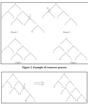
are replaced with individuals and establishes branches of a tree. Random changes are happened via replacement of the operators in the programs, changing value of a knot or replacement of the branches of the trees with each other [15,16]. Figure 1 shows three examples of GPs as trees.
The main characteristic of the GP algorithms is that they need a large population with thousands or even mil- lions of individuals. Therefore, these algorithms are usu- ally very slow and because of working on the basis of trees, more individuals in the population, more efficient and faster algorithms are obtained [14]. However, in general case, attaining a desired fitness value is very time consuming, but this is not very horrific because with one time of running the algorithm, a model attains which could be used simply for the problem. Another special characteristic of the GP is that, the answer is a model instead of a value which may be nonlinear. In addition to these aspects, in the standard form of GA, the lengths of chromosomes are constant, but in the GP algorithm these lengths might be variable. In the GP algorithm the first step is to make the first generation by creation of random programs. Each program has a fitness value that deter-mines the chance of the program in the creation of the next generation. In the GP algorithms, two main opera-tors which are necessary to make the next generations are crossover and mutation.
In the crossover process, a child program is made by changing the random parts of two selected parents. As shown in Figure 2, point C of the parent 1 and point D of the parent 2 are selected for the crossover process, and then the outcome children of such process are drawn. The mutation process in which, a child program is modi- fied by altering a randomly selected part, is a guarantee for the existence of versatility in the population of a gen- eration. An example of such process is shown in Figure 3 where, the mutation has been done in point C. A sche- matic flowchart for the creation of the generations in the GP algorithm is shown in Figure 4. At the present study, a GP model is proposed for the prediction of concrete faced rock fill dams settlements considering different variables that affect the results and the domain in which these variables changes. It is noteworthy that using the GP algorithms does not guarantee obtaining the most optimum result but it allows achieving an approvable result in a reasonable calculating time.
X
X
X
X X
+ - +
* *
1 1
2
[image:4.595.324.517.651.719.2]X+1 (X*X)-1 X+(X*2)
a *
3 3
*
+
+ +
-/ *
2
3 y
x +
y +
12 1
y y
C
D
+
-*
2
3 y
x +
a *
3
3 *
/
y +
12 1
Parent 1 Parent 2
Child 1 Ch
+
+
y y
[image:5.595.145.446.78.432.2]ild 2
Figure 2. Example of crossover process.
+
-/ *
2
3 y
x +
y +
12 1
C
+
-*
2
3 y
x +
x
-3 a *
3
Figure 3. Example of mutation process.
with p_ select variation op.
probabilistically no
with p_
select one individual select
perform mutation perfo
i= i+1
add inter add offspring to
intermediate pool
i= population size?
two individual
rm crossover
i= i+2
next generation yes
offspring to mediate pool
Figure 4. A schematic flowchart for the creation of gene- rations in the GP algorithm.
3.2. Initial Information for the GP Model
Paying attention to the information in Table 1, it can be seen that big differences exist between the times when settlements are measured. It is also perceived that the settlement would reach to a moderately persistent amount about 6 years after construction of the CFRs, so informa- tion of settlement before this age is not invokable. Ac-
cording to this, information of 5 dams includes Man- grove Greek, Tianshengiao, Ita, Janheung and Daegok has been ignored and information of 30 other dams has been used. The range of changes in the height and length of these dams are 26 - 187 m and 110 - 1168 m respec- tively. The input variables which are used for the predic- tion of the settlement are shape factor (SF), void ratio (e), height (H) and vertical deformation modulus (Ev) of dams. Table 4 shows the range at which these input pa-rameters changes.
3.3. The GP Model for the Prediction of Dams Crest Settlements
A GP model is constructed on the basis of 67 percent of the all existing data (information of 21 dams of all 30 dams). The remaining information (the remaining nine dams) has been used for testing the model. The overall characteristics of the algorithm are presented in Table 5.
After training and using the above information, the model is finalized as follows:
* cos cos ln cos co
R D Sc H s 66Sc
* * ln ln
R I e Sc H Sc H 384
ln 0.2837 cos cos cosA 0.1435
ln H H H 20 cos cos ln 13 B
A
0.1367
^ 2 2.4849 Vc H
20 cos ln
11 ln 11 ln
ln 0.0136 3.1416
C H
Sc Sc S
i E
ln
Sc H
ln V 11.02 ln cos
D E C H
20
D ln 11 cos ln E Sc B H
ln 12
cos cos 66
V
FE E H Sc 11
cos 0.1367G G
cos cos ln 13 20 cos cos 11 Sc
* 11 0.9983 0.9983I F G ScJ
K
2
20 cos ln cos 107.138
20 cos ln cos 11
ln 11 V ln
Sc H
I G H
E Sc H
A
* 20 cos ln 11 * 0.6805
B H Sc A
ln V 11 ln ln 0.9983
M E Sc H L
0.0.78 0.543
N
Sc
ln 0.2837 H cos cos 1.792 H
cos cos ln 13 20 cos 0.1 O N 367
Sc
M O
* ln 20 cos ln 11C H
cos 66 Sc
C*
ln V 11 ln 12 cos P E H
H 0.1367
cos cos ln 13 20 cos cos 11
Q
* ln 11
D K Sc P Q
cos cos 66
S H Sc
ln ln 12
11 Sc ln
Sc H
cos cos ln 13 ln 12 0.5735
T H e
20
U Sc S T
* ln 13 ln 12 cos cos 66
E H Sc
2 *
ln V 11 cos cos 16
V E Sc E
ln cos 198
W U V H Sc H
* ln cos cos 66 F Sc H Sc
*
cos cos 13 cos cos
X W F
ln V 11 ln cos cos V
Y Sc E X Sc H E
ln cos ln 0.96 0.5402 3.1416
96
Z H i Y
Sc
* cos cos ln
G Z Sc H c
* ln cos cos 6 ln 48
H e Sc H Sc Sc H
*
* ln 0.2837 cos cos 11 4.344
Cc G
H H H
* ln cos cos cos 77
[image:6.595.311.538.494.585.2]I Sc H CC Sc
Table 4. Range of input parameters changes. Range were considered Input variable
26 - 187 (m) Dam height (H)
0.17 - 0.4 Void ratio (e)
25 - 375 (MPa) Vertical deformation modulus
after construction (EV)
[image:6.595.312.537.613.733.2]0 - 34.6 Shape coefficient (Sc)
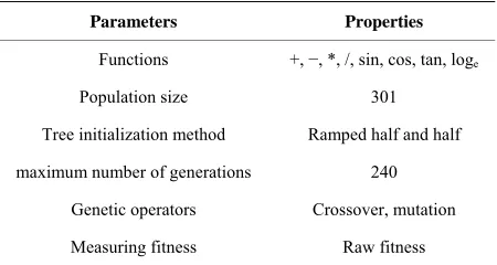
Table 5. The overall characteristics of the GP algorithm.
Parameters Properties
Functions +, −, *, /, sin, cos, tan, loge
Population size 301
Tree initialization method Ramped half and half
maximum number of generations 240
Genetic operators Crossover, mutation
The number of knots in the model is 701 and its depth is 50. The results indicate that; there is a good agreement between the results and measured settlements with cor-relation factor of 0.98, and a proper performance for the model in the testing stage is achieved.
4. The Verification of the Trained Model
With training the model, and to demonstrate the effi-ciency of the algorithm for the prediction of the CFRDs settlements, information of 9 dams is used for the testing. To verify the trained model, the results obtained are compared with the findings of the Clements method. The reliability of the model and predicted values for the crest settlement obtained in the present work and the ones ob-tained by the Clements method is shown in Figure 5.
Table 6 shows the mean, standard deviation and the minimum least square error values between the measured values (using Clements model) and those obtained by present GP model. The results indicate that; even though the statistical analysis is derived from a limited set of information, however the performance of the present GP model is better in comparison with the Clements model. Due to the lack of physical model for testing and meas-urement of the crest settlement and for complex phe-nomena, it seems that; the presented GP algorithm has the capability for prediction of dam crest settlement.
5. Comparison between the GP and Finite
Element Models
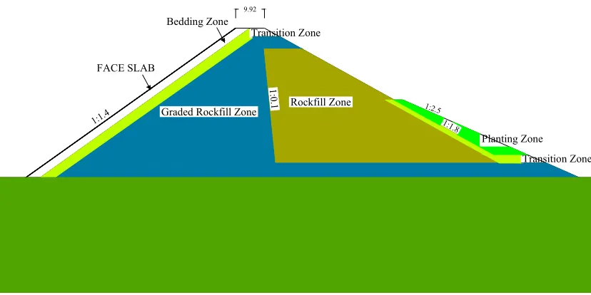
To evaluate and compare the results obtained by the GP and finite element models, the Daegok earth dam is modeled using the presented GP model and PLAXIS method. Daegok dam is a CFRD type dam with 52 m in height. The dam crest length and width are 190 m and 9.5 m respectively. The total volume of its body is 479 m3. The slope of the upstream face is 1V:1.4H, and for the downstream face is 1V:1.8H. The details of the dam sec-tion and construcsec-tion procedures are shown in Figure 6 and Table 7 [9]. Tables 8 and 9 present the overall specifications of soils used in the dam model. Due to using rock material in the dam body, a hardening hyper-bolic soil model is used for the analysis. It is assumed that the soil is homogenous in all cases. Table 8 de-scribes the common properties of the Mohr-Coulomb and hardening models, while Table 9 contains complemen-tary parameters belong only to the hardening model.
There are 14 computing phases in the Plaxis model. The first phase is considered for applying initial stresses. Due to slope existence, the gravity loading method is used. The other 13 phases are considered for modeling of the layered soils and three impounding steps of 15, 30 and 40 meters levels. Using this model, the long term settlement for the dam crest is 7.9 cm, while the dam
settlement at the end period of construction is about 3 cm, which is shown in Figure 7. Using Equation (1), for a point located near the dam crest, the vertical deformation modulus (Ev) is determined 138.8 MPa at the end of con-struction period as follow:
3
4 48 21.5 138.8 MPa 140 MPa 1000 29.75 10
v
E
(4)
At this stage, using Equation (3) and the values of e = 0.25, H = 52 m, Sc = 3.7, and Ev = 140 MPa, the dam crest settlement is predicted by the GP model, which is equal to 7.8 cm. This finding is very close to the ones obtained by the finite element method. The results con-firm the liability of the presented GP model.
6. Conclusions
In the present study which focused on the prediction of earth dam crest settlement using the genetic program
Figure 5. The results of present GP model in comparison with the Clements model.
Table 6. Statistical comparison between the present GP model and Clements model.
Model RMSE average error Absolute Absolute standard deviation error
The present GP
model 0.132 0.082 0.109
Clements theory 0.307 0.15 0.285
Table 7. The construction time-table of Daegok Dam [9].
Main construction process
Period Explanation
2001.9 - 2002.4 Completion of dam embankment (52 m) for 8 month
2002.4 - 2003.3 Stabilizing period and shotcrete on upstream slope for 12 months
2003.3 - 2003.5 Construction of the face deck, 3 months
1:0.1
1:1.4 1:1.8
1:2.5 Rockfill Zone
Graded Rockfill Zone
Planting Zo Tr Transition Zone
Bedding Zone
FACE SLAB
ne
ansition Zone
[image:8.595.85.499.85.292.2]9.92
[image:8.595.83.517.294.528.2]Figure 6. The Daegok dam cross section.
[image:8.595.59.541.576.733.2]Figure 7. The crest settlement after dam construction.
Table 8. Properties of soil in the hardening and Mohr-Coulomb models.
Soil Model γ (kN/m3) Young’s modulus (kN/m2) Poisson’s ratio Cohesion (kN/m2) Friction angle Void ratio
Face bedding Mohr-Coulomb 22.7 3 × 10⁴ 0.35 0 45 0.30
Face slab Mohr-Coulomb 22.0 2 × 10⁷ 0.30 150 27 0.50
Foundation Mohr-Coulomb 22.0 2 × 10⁷ 0.30 150 27 0.50
Graded rock-fill Hardening model 21.5 - 0.30 0 45 0.25
Planting Mohr-Coulomb 18.0 3 × 10⁴ 0.35 1 35 0.30
Rock-fill Hardening model 20.3 - 0.30 0 39 0.25
Transition Mohr-Coulomb 21.5 3 × 10⁴ 0.30 0 45 0.30
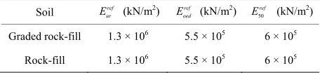
Table 9. Special properties for the soil hardening model.
Soil ref
ur
E (kN/m2) ref oed
E (kN/m2)
50
ref
E (kN/m2)
Graded rock-fill 1.3 × 10⁶ 5.5 × 10⁵ 6 × 10⁵
Rock-fill 1.3 × 10⁶ 5.5 × 10⁵ 6 × 10⁵
ming model the following conclusions are made:
1) The results obtained by the GP model is in agree with the ones calculated through the experimental meas-urements.
2) The GP model, which is based on four characteris-tics of: Ev, H, e, and Sc has the best applicability and is in contrast with conventional methods such as Clements method, which only uses the H parameter for estimation of the crest settlement.
3) The results obtained by the GP model have a good compatibility with the finite element modeling.
4) The GP model is a trained model, and is capable of calculating the dam crest settlement without using any field laboratory tests.
5) The GP model can be used for complex problems, where rock-fill with various settlement aspects are in-volved.
6) Even though, the GP model is derived from a lim-ited set of information and is not necessarily the most perfect one, however, the performance of this model is better in comparison with the conventional models such as: the Clements model.
7) The main weakness of the GP modeling is the time consuming and the needs for a huge population, but when the model is trained, many complex aspects can be predicted.
REFERENCES
[1] G. Hunter and R. Fell, “The Deformation Behavior of Rokfill,” Uniciv. Report No. 405, The University of New South Wales, Sydney, 2002.
[2] F. Saboya, R. Barosa and A. Vasconcelos, “The Influence of the Left Abutment Geometry on the Behaviour of Xingo Rock-Fill Dam,” Proceedings of the International Symposium on Concrete Faced Rock-Fill Dams, Beijing, 18 September 2000, pp. 565-572.
[3] G. F. Sowers, R. C. Williams and T. S. Wallace, “Com-pressibliity of Broken Rock and the Settlement of Rock-fills,” Proceedings of the 6th International Conference on Soil Mechanics and Foundation Engineering, Toronto, Vol. 2, 1965, pp. 561-565.
[4] F. L. Lawton and M. D. Lester, “Settlement of Rockfill
Dams,” Proceedings of the 8th International Congress on Large Dams, Edinburgh, Vol. 3, 1964, pp. 599-613. [5] C. Soydemir and B. Kjaernsli, “Deformations of
Mem-brane-Faced Rockfill Dams,” Proceedings of the 7th Eu-ropean Conference on Soil Mechanics and Foundation Engineering, Brighton, Vol. 3, 1979, pp. 281-284. [6] R. P. Clements, “Post-Construction Deformation of
Rock-fill Dams,” Journal of Geotechnical Engineering, Vol. 110, No. 7, 1984, pp. 821-840.
doi:10.1061/(ASCE)0733-9410(1984)110:7(821)
[7] M. D. Fitzpatrick, B. A. Cole, F. L. Kinstler and B. P. Knoop, “Design of Concrete-Faced Rockfill Dams,” In: J. B. Cooke and J. L. Shererd, Eds., Concrete Face Rockfill Dams-Design, Construction, and Performance, 1985, pp. 410-434.
[8] N. L. S. Pinto and P. L. M. Filho, “Estimating the Maxi-mum Face Slab Deflection in CFRDs,” Hydropower & Dams, Vol. 5, No. 6, 1998, pp. 28-30.
[9] P. Han-Gyu, S. Min-Woo, K. Yong-Soeng and L. Heiu- Dae, “Settlement Behavior Characteristics of CFRD in Construction Period-Case of Daegok Dam,” Journal of the KGS, Vol. 21, No. 7, 2005, pp. 91-105.
[10] N. Kovacevic, “Numerical Analyses of Rockfill Dams, Cut Slopes and Road Embankments,” Ph.D. Thesis, Im-perial College of Science, Technology and Medicine, London, 1994.
[11] J. M. Duncan, “State of the Art: Static Stability and De-formation Analysis,” ASCE Geotechnical Special Publi-cation, Vol. 1, No. 31, 1992, pp. 222-266.
[12] J. M. Duncan, “State of the Art: Limit Equilibrium and Finite-Element Analysis of Slopes,” ASC.E Journal of Geotechnical Engineering, Vol. 122, No. 7, 1996, pp. 577-595.
doi:10.1061/(ASCE)0733-9410(1996)122:7(577) [13] Y. S. Kim and B. T. Kim, “Prediction of Relative Crest
Settlement of Concrete-Faced Rockfill Dams Analyzed Using an Artificial Neural Network Model,” Computers and Geotechnics, Vol. 35, No. 1, 2008, pp. 313-322. doi:10.1016/j.compgeo.2007.09.006
[14] Y. Zhang and S. Bhattacharyya, “Genetic Programming in Classifying Large-Scale Data: An Ensemble Method,” Information Sciences, Vol. 163, No. 1-3, 2004, pp. 85- 101.doi:10.1016/j.ins.2003.03.028
[15] J. R. Koza, “Genetic Programming: On the Programming of Computers by Means of Natural Selection,” 6th Print-ing, Massachusetts Institute of Technology, Cambridge, 1998.
![Table 1. Performance and structural properties of CRFDs [13].](https://thumb-us.123doks.com/thumbv2/123dok_us/9289613.424616/3.595.63.537.114.734/table-performance-structural-properties-crfds.webp)
![Table 3. Comparison of measured and estimated settle- ments values [13].](https://thumb-us.123doks.com/thumbv2/123dok_us/9289613.424616/4.595.58.282.187.732/table-comparison-measured-estimated-settle-ments-values.webp)