The sampling brain

(1)

warwick.ac.uk/lib-publications

A Thesis Submitted for the Degree of PhD at the University of Warwick

Permanent WRAP URL:

http://wrap.warwick.ac.uk/132094

Copyright and reuse:

This thesis is made available online and is protected by original copyright. Please scroll down to view the document itself.

Please refer to the repository record for this item for information to help you to cite it. Our policy information is available from the repository home page.

(2)

The Sampling Brain

by

Jian-Qiao Zhu

A thesis submitted in partial fulfilment of the requirements for the degree of Doctor of Philosophy in Psychology

Department of Psychology University of Warwick

December 2018 M

A E

G NS

IMOLEMT A T

U N

IV

ERS_{ITAS WARWI}CEN

(3)

[image:3.595.119.469.147.767.2]

List of Figures

Section Caption Page

1.1 2

2.5a 21

2.5b 23

2.5c 27

An example of searching behaviours in a 2D patchy environment. Each patch could represent a cluster of animal names. Repeated simulation of samplers in different environments can be found in

Figure 3. (Left Panel) Simulation result for DS. The top panel shows the trajectory of the first 100 positions (red dots). The bottom panel shows the log-log plot of flight distance distribution. The raw histogram of flight distance is also included in the bottom panel. The power-law exponent is fitted using LBN method, which corrects for

irregular spacing of points (Rhodes & Turvey, 2007). (Middle Panel)

The same treatments for RwM sampler. The Gaussian proposal distribution was an identity covariance matrix. (Right Panel) The

same treatments for ! sampler with 8 parallel chains and only the

positions of the cold chain were displayed here. The Gaussian proposal distributions for all 8 chains had the same identity covariance matrix. For all three samplers considered here, only the first 1024 samples were used to match the length of human experiments.

MC3

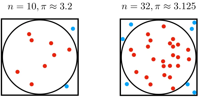
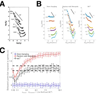
Approximating the value of ! through sampling. Points that placed inside the circle were marked as red and those outside were blue. The accuracy of sample-based approximation increases with more samples scattered in the square, on average.

π

(A) Estimates of time duration show 1/f noise. The target durations for participants to estimate are shown next to scatterplots and the target duration ranged from 10s (top) to 0.3s (bottom). Best fit

power-law exponents to the power spectra are ! , and this is also

the range shown in dashed lines in Figure 4C. Figure was adapted from Gilden et al. (1995). (B) Power spectra produced by DS (left),

RwM (middle), and ! (right). Only ! with 8 parallel chains can

generate 1/f noise. For all the sampling algorithms, the first 1024

samples were used. (C) Estimated power-law exponent in power

spectra are related to the ratio between Gaussian width and proposal step size. The power-law exponents for power spectra (! ) were fitted following methods suggested by (Gilden et al., 1995; Gilden, 1997). The dashed lines show the range of ! suggested by Gilden et al.

(1995). Error bars indicate ! SEM. When the ratio is low the

acceptance rate of proposed sample should be low; it is the opposite case for the high ratio. The asymptotic behaviours of ! are 1/f

noise, of RwM are brown noise, and of DS are white noise.

α ∈[0.90,1.20]

MC3 MC3

̂

α

1/fα

±

MC3

(A) Animal naming task as non-destructive mental foraging (10

participants). The estimated power-law exponents for IRI are

! . (B) Estimated power-law exponents for flight distance

distributions for the three sampling algorithms across different patchy environments, manipulating the spatial sparsity of the Gaussian mixtures. The dashed lines show the range of power-law exponents

suggested by our human data. Only ! falls in this range. (C) KL

divergence of mode visiting from the true distribution for the three

sampling algorithms. Red denotes RwM, black denotes ! , and blue

denotes DS. The patchy environments are the same for all three algorithms. The quicker the sampler approaches zero KL divergence, the better the sampler is searching the patchy environment. The solid

lines are medians of the dashed lines. (D) Simulated standard MCMC

with power-law proposal distribution. The solid line shows the median in estimated power-law exponent. The dashed lines show the range of human data.

μ ∈[.77,2.39]

MC3

(6)

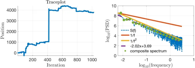
2.7a Autocorrelations produced by a Lévy flight. (Left) The trace plot of

first 1024 locations of the Lévy flight. (Right) The power spectra of

the locations.

33

2.7b 34

2.7c 35

3.8 51

3.9 An illustration of model behaviours. The relationship between the true

probability (x-axis) and the expected probability estimates (y-axis) predicted by the probability theory plus noise model (left) and the sampling plus correction model (right).

57

3.10 The relationship between the mean and the variance of people’s

probability estimates (left panel: Costello et al., 2018; right panel:

Stewart et al., 2006). (A) The sampling plus correction model predicts

a quadratic relationship (purple lines). (B) The probability theory plus

noise model predicts a constant relationship (purple lines). Best-fitted model parameters are displayed in the titles, and the MSE of each

model in predicting the empirical tasks can also be found in the Table

5.

60

3.12 The degree of improvement in the probability estimate (y-axis) due to

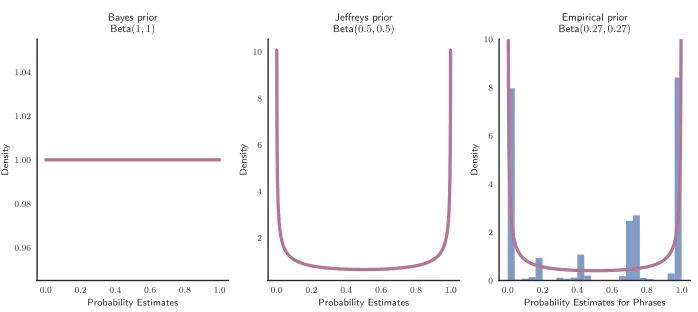
the inclusion of the correction step in the sampling plus correction model. X-axis depicts the true probability distributions from Beta(0.1,0.1) (most left) to Beta(10,10) (most right). An empirical prior, Beta(0.27,0.27), was used in the correction step as explained in the text.

68

4.2 Schematic of the random replay model. The standard error-correction

learning rule is depicted in solid arrows. In addition, the model assumes a memory of past trials, which are then randomly sampled and then replayed (dashed arrows). The replayed trials are treated like any other trial and are used to update associative strength through the standard error-correction learning rule.

74

4.3a Spontaneous recovery predicted by the random replay model (blue),

whereas the classic Rescorla-Wagner model (red) predicts no recovery in the third phase. Both models are repeatedly simulated for 100 times with exact same set of parameters. The median value of these simulated runs are depicted as solid lines.

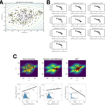
79 (A) 2D semantic space of all animal names. Each dot denotes one animal name. The contour represents a Gaussian mixture model on

these animal names. (B) Histogram of flight distances for 10

participants from the animal naming task. The estimated power-law

exponent ! . Median correlation coefficient between the

flight distance and IRIs is 0.19. (C) Running three sampling

algorithms on the Gaussian mixture model from B. As shown above,

only the ! can replicate the power-law scaling of flight distance in

the semantic space.

̂

μ∈[0.76,1.28]

MC3

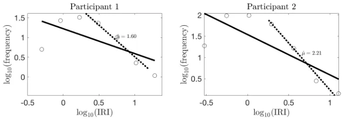
Histogram of IRIs (log-log plot) for two participants in noun-recall task. The estimated power-law exponents for the tail distribution are

! ̂ (participant 1) and ! (participant 2).

μ = 1.60 μ̂= 2.21

Illustrations of the Bayes prior (left), the Jeffrey prior (middle), and an empirical prior (right). The empirical prior was obtained by fitting the histogram of the normalised frequencies (adjusted by the proportion of uses) of the probability-describing phrases in natural language against the mean probability estimates of the same phrases (British National Corpus; adapted from Stewart et al., 2006, Table 2). The purple curve shows the best-fitted symmetric Beta distribution:

! .

(7)

4.3b 80

4.3c The random replay model of classical conditioning for both normal

and hippocampal lesion animals. The learning phenomena were in figure title and the simulated experimental procedures were separated

by dashed lines. (A) Spontaneous recovery. (B) Latent inhibition. (C)

Backward blocking. (D) Recovery from overshadowing. (E) Recovery

after blocking. All simulations presented here used the exact same set

of model parameters in main text and also for Figure 9 and 10 above.

83

5.2 Formal representation of the information-choice task as a Markov

Decision Process (MDP). Two offers (red and blue circles) are presented, and the animal must choose one of them. A cue then appears after this initial choice (Initial Link: IL), which is either informative (green S+ indicates a rewarding outcome; yellow S0 indicates a neutral outcome with probability q and 1-q respectively) or uninformative (black S* leaving the animal in a state of uncertainty). Following a delay (Terminal Link: TL), the animal obtains the outcome (reward or no reward). The anticipatory signals proposed by the APE model are illustrated as the purple dashed lines.

93

5.4a Schematic illustration of the four-phase information-seeking task in

Stagner & Zentall (2010). In the Training phase, pigeons learned to prefer the cued option (depicted as “Left”). Then the cue-outcome contingency was reversed in the Reversal phase, and pigeons still learned to prefer the cued option (now “Right”). In the third

Discrimination phase, novel choice stimuli (“Circle” and “Plus” shapes) were introduced while keeping the same cue-outcome contingency. The shapes were counterbalanced across pigeons, and they again learned to prefer the cued option (“Plus” in this case). In the final Non-Discrimination phase, choosing either option should not provide valuable advance information, and pigeons learned to prefer the one with the higher expected value (“Plus” in this case).

99 Shorter acquisition-extinction interval have greater degree of

spontaneous recovery. (A) Experimental data with pigeon subjects.

Responses that had been trained distantly from (! : longer

acquisition-extinction interval) or proximally to (! : shorter acquisition-extinction

interval) extinction. ! exhibits greater recovery than ! in recovery

test. The figure was adapted from Rescorla (2004). (B) Simulation of

the random replay model. The Rescorla (2004) experiment has five phases (left to right: ! +, ! +, random mixture of ! - and ! -, rest,

and test). The random replay model predicts that ! emerges to

recover more than ! .

R₁ R₂

R₂ R₁

R₁ R₂ R₁ R₂

(8)

5.4b 103

5.4c 105

5.4d 109

The effect of uncertainty reduction on choice of the informative option. (A) Illustration of the experimental procedure used in Green & Rachlin (1977) to study pigeons’ preference for uncertainty reduction.

Both options had the same probability of reinforcement (p), but after

choosing the cued option pigeons were informed of the eventual outcome immediately from the colour signals. Choosing the uncued option, however, left pigeons in a state of uncertainty until the end of trial (30 s later). The tested values of p changed across the range of

4%, 10%, 20%, 40%, 50%, 60%, 80%, 90%, 96%, and 100%. (B)

Experimental data from Green & Rachlin (1977) are in black, and error bars indicate ! SEM. The simulations of the TD model (blue)

and APE model (shades of red for different ! parameter). The

softmax inverse temperature and discount factor were ! .

The APE model can reproduce the quadratic relationships observed in data.

±

w+

β = 6, γ = .98

(A) Behavioural data from the four-phase task of Stagner & Zentall (2010). Strong preferences for advance information and lower reinforcement rate option emerged through experience in the Training, Reversal, and Discrimination phases. When the advanced information is absent (Non-discrimination phase), pigeons learnt to choose the option with the higher reinforcement rate. The figure was adapted from Stagner & Zentall (2010). (B) The TD model predicts no preference for advance information. Value functions were initialised at 0. At the first trial in the Reversal phase, cue values were reset to 0 to account for changes in cue-outcome contingency. At the first trial in the Discrimination phase, value functions were agin reset to 0 for the

new choice context. (C) The APE model can capture the dynamics of

choice probability of the suboptimal option with advanced information. The same simulated procedure was used as for the TD model. We set the learning rate, inverse temperature in the softmax

choice rule, and the discount factor at ! for

both models. The APE model has an additional parameter: the

sampling bias for good news, which was set at ! . Both the TD

and APE model were repeatedly simulated with the same set of parameters 100 times, and the solid lines denote the median of individual simulated run (dashed lines).

α= .06, β = 6, γ = .98

Δw = 4

Delay to outcome manipulation in the information-choice task. (Left)

The pigeon study found that longer delays induce greater preference for the cued option (Spetch et al., 1990). The experiment contained a cued option with 50% reinforcement rate and an uncued option with 100% reinforcement rate. The durations of the TL was varied across

5, 10, 30, 50, and 90 seconds. (Right) The human study found a

similar pattern (Iigaya et al., 2016). Both the cued and uncued option had a 50% reinforcement rate. The TD model fails to reproduce the increase in preference for cued options with an increase in TL, whereas the APE model successfully captures this relationship. We set the inverse temperature in softmax and the discount factor

! for both models. The APE model has an additional

parameter ! .

β = 2, γ = .98

(9)

5.4e 111

5.4f People preferred advanced information, but less so when aversive 113

outcomes were included in the gamble. (A) Experimental procedure

of the human information-choice task reported in Zhu et al. (2017). Participants chose between an informative “Find Out Now” option and a non-informative “Keep It Secret” option. By choosing the informative option, participants could know immediately the nature (appetitive, aversion, or neutral) of upcoming images by inference from the animal symbols. By choosing the non-informative option, however, the same animal symbol always appeared, and the final outcome was only revealed at the end of trial. The diagram only depicts the Good condition, which contains 50% erotic and 50% neutral images. We also tested a Bad condition (50% aversive and 50% neutral images) and a Mix condition (50% erotic and 50% aversive

image). (B) The time series of choice probability for the informative

option (i.e., “Find Out Now”). Shaded area indicates ! SEM. (C)

Predicted time series of choice probability from the TD model. The model was repeatedly simulated 100 times with the same set of parameters (dashed lines). The solid lines are the median of the dashed lines. At asymptote, the TD model chooses indifferently

between the two options. (D) Similar simulations from the APE

model. The asymptotic behaviour of the APE model agrees with the human data. Both models share the same learning rate, inverse

temperature, and discount factor ! . For the

APE model, additional sampling weights parameters were used, as displayed in the figure legend.

±

α = .06, β= 3, γ = .98

Reward magnitude manipulation. (A) An illustration of the

experimental procedure of the monkey study reported in Blanchard et al. (2015). On each trial, monkeys were presented with two offers in sequence, each followed by a dark screen period (order is counterbalanced). Then they had to choose between a cued offer (cyan bar) and an uncued offer (magenta bar). The height of the central white bar indicated the amount of liquid potentially available on that trial, and the green and red dots revealed whether the risky option won or lost respectively. The probability of reinforcement for both options was 50% throughout experiment. After a 2.25s cue

presentation, the monkeys received outcome delivery. (B) Behavioural

results. Preference for the cued option as a function of the liquid amount difference between the cued and uncued options. Error bars indicate ! SEM. The figure is adapted from Blanchard et al. (2015).

(C) Predictions of the TD and APE model. We set the inverse

temperature and discount factor as ! for both models.

The APE model has an additional sampling weights parameter as shown in the figure legends.

±

(10)

List of Tables

Section Title Page

2.3 Empirical evidence for Lévy flights and 1/f noise in human mental

samples. 17

3.7 Summary of combined probability expressions tested by Costello &

Watts (2014) and Costello et al. (2018). 49

3.9 Summary of model predictions (left to right: probability theory,

probability theory plus noise model, sampling model, Bayesian sampling model) on the average values of the combined probability

expressions from Table 1.

58

3.10a Predicted variance of human probability estimates from the

Probability Theory plus Noise model and the Bayesian sampling model.

59

3.10b Fitting results for both the probability theory plus noise model and

the sampling plus correction model. 61

4.3a All types of classical conditioning trials considered in this Chapter.

CS1 and CS2 denotes two different conditioned stimuli. US denotes the unconditioned stimulus.

76

4.3b Experimental procedures in classical conditioning. 77

5.4 Key experimental variables that found to determine the preferences

(11)

Acknowledgements

I am fortunate to have many people to thank.

My primary advisor, Elliot Ludvig, for the opportunity to conduct researches in psychology. My interests in computational modelling were kindled at his neuroeconomics course. Later, I spent a summer building cognitive models using reinforcement learning algorithms, and since then, he has been instrumental in guiding me and demonstrating the power of reverse-engineering the mind.

My second advisor, Adam Sanborn, for the right balance of freedom and guidance, for all the late night email chains, for his careful and critical reading of manuscripts, and for the most intensive and productive collaborations at Warwick. Adam brings excitements to all the mathematical and research problems, and his works inspired me to explore rational analysis and Bayesian models.

I would like to acknowledge a debt to Nick Chater, certainly an unofficial advisor, for his inspiration all along the way, for his helpful advises on research and career, and for showing me, along with a generation of students and readers, the power of theory.

I also owe a great deal to Samuel Gershman and his students, Ishita Dasgupta, Eric Schulz, and Rahul Bhui, for their friendly reception at Harvard and for many enlightening discussions.

My experience as an international graduate student would have been poorer but for the fellow students at Warwick and the friends around the world. For their friendships and for many selfless supports, I would like to particularly thank Andong Chen, Victoria Collard, Ahuti Das, Tianshi Feng, Alina Gutoreva, Daniel Gunnell, Anita Lenneis, Chao Li, Ling Liu, Si Li, Wenfeng Li, Danielle Norman, Max Rodriguez, Divya Sukumar, Wonnie Sim, Alexandra Surdina, Mengran Wang, Wendi Xiang, and Shengnan Zhang.

(12)

Declaration

This thesis is submitted to the University of Warwick in support of my application for the degree of Doctor of Philosophy. It has been composed by myself and has not been submitted in any previous application for any degree. The work presented (including data generated and data analysis) was carried out by the author except in the cases outlined below.

Inclusion of Published Works

Parts of this thesis have been published or preprinted by the author. Chapter 2 includes the following publication:

Zhu, J. Q., Sanborn, A. N., & Chater, N. (2018). Mental Sampling in Multimodal

Representations. In S. Bengio, H. Wallach, H. Larochelle, K. Grauman, N.

Cesa-Bianchi, & R. Garnett (Eds.), Advances in Neural Information Processing

Systems (pp. 5749-5762). Montréal, Canada.

JQZ, ANS, and NC designed research; JQZ and ANS derived the models and analysed the data; JQZ carried out model simulations and data analyses; JQZ and ANS wrote the manuscript in consultation with NC. ANS supervised the project.

Chapter 3 includes the following preprint:

Zhu, J. Q., Sanborn, A. N., & Chater, N. (2018, November 28). Bayesian inference causes incoherence in human probability judgments. https://doi.org/ 10.31234/osf.io/af9vy.

JQZ, ANS, and NC conceived of idea and developed the theory; JQZ performed the data analysis and model simulations; All authors discussed the results and contributed to the final manuscript. ANS supervised the project.

Chapter 4 includes the following preprint:

Ludvig, E. A., Zhu, J. Q., Mirian, M. S., Kehoe, E. J., & Sutton, R. S. (under review).

Associative learning from replayed experience. On bioRxiv, 100800.

EAL, JQZ, MSM, EJK, RSS conceived of idea and developed the theory; EAL, JQZ, and MSM performed model simulations; EAL and RSS encouraged JQZ to investigate new memory model and hippocampal lesion data; All authors discussed the results and contributed to the final manuscript. EAL supervised the project.

Chapter 5 includes the following publications:

(13)

JQZ and EAL conceived of idea and developed the theory and experiment; WX conducted experiments and collected data; JQZ and WX analysed behavioural data; JQZ performed model simulations; All authors discussed the results and contributed to the final manuscript. EAL supervised the project.

Rodríguez-Cabrero, J. A. M., Zhu, J. Q., & Ludvig, E. A. (2019). Costly curiosity:

People pay a price to resolve an uncertain gamble early. Behavioural

Processes.

(14)

Abstract

(15)

Abbreviations

Abbrev. Explanations

MCMC Markov chain Monte Carlo

Metropolis-coupled Markov chain Monte Carlo

IRI Inter-response interval

DS Direct Sampling

KL Kullback-Leibler

AR Auto-regressive

RF Relative frequency

PTN Probability Theory plus Noise

BS Bayesian Sampling

ESS Effective sample size

MSE Mean squared errors

CS Conditioned stimulus/stimuli

US Unconditioned stimulus/stimuli

MDP Markov decision process

RL Reinforcement learning

IL Initial link

TL Terminal link

TD Temporal difference

APE Anticipated prediction errors

!

(16)

(17)

Chapter 1 Why Sampling?

“The first thoughts and attempts I made to practice [the Monte Carlo method] were suggested by a question which occurred to me in 1946 as I was convalescing from an illness and playing solitaires. The question was what are the chances that a Canfield solitaire laid out with 52 cards will come out successfully? After spending a lot of time trying to estimate them by pure combinatorial calculations, I wondered whether a more practice method than ‘abstract thinking’ might not be to lay it out say one hundred times and simply observe and count the number of successful plays” (Stan Ulam, 1983)

1.1 Intuitions for Sampling

The spirit of sampling is captured by Stan Ulam’s interest in estimating the probability of winning in solitaire — from the simple to the sublime. When the analytical solution is difficult to obtain, numerical approximations are often treated as desirable alternatives. Another classic example that demonstrates the power of sampling is the calculation of the value of ! (the ratio of a circle’s circumference to its diameter). The sample-based approximation to ! takes three simple steps. First, we inscribe a circle within a square. Second, randomly scatter a number of points over the square. Third, count up the number of points bounded inside the circle. Given that the ratio of areas of circle and square is ! , the value of ! can be approximated from number of points inside the circle and the total number of points:

! (1.1)

As illustrated in the Figure 1, on average, the sample-based approximation improves in accuracy to the true value of ! as more samples are generated.

π

π/4 π

π ≈4× no. of_total points_no. _ofwithin_points circle

(18)

[image:18.595.131.470.261.429.2]

Indeed, the history of scientific development resembles an ever-lasting sample-based approximation to truth. Generations of scientists are constantly drawing samples from nature, through experimentation, in order to perform better estimates on the probabilities of possible theoretical models. Though the number of samples or experiments is always finite, by continually sampling, we slowly build up a picture of all of the probabilities.

Figure 1. Approximating the value of ! through sampling. Points that placed

inside the circle are marked as red and those outside are blue. The accuracy of sample-based approximation increases as more samples are scattered in the square, on average.

1.2 A Rational Model of Sampling Brain

Similar challenges, at least in principle, are also imposed on the brain: the world is a highly uncertain place, and we want our brain to be able to generate good estimates of these uncertainties. In fact, there are many sources of uncertainty the brain has to deal with, including the sensory system, the motor apparatus, one’s own knowledge, and the data-generation process from the world. To process noisy data efficiently to make judgments and guide choices, the brain must represent and use information

π

(19)

about uncertainty in its computations. One normative and ecologically rational method is for the brain to adopt a Bayesian approach because it provides an optimal way of reasoning about these uncertainties — the

Bayesian brain hypothesis (Knill & Pouget, 2004; Doya, Ishii, Pouget, & Rao, 2007; Friston, 2012; Sanborn & Chater, 2016). Indeed, over the past few decades, Bayesian approach has spawned an enormous range of applications in cognitive science from perception (Knill & Richards, 1996; Yuille & Kersten, 2006; Gershman, Vul, & Tenenbaum, 2009; Shams & Beierholm, 2010), memory (Anderson & Milson, 1989; Gershman, 2017), intuitive physics (Sanborn, Mansinghka, & Griffiths, 2013; Battaglia, Hamrick, & Tenenbaum, 2013), and animal learning (Courville, Daw, & Touretzky, 2006; Gershman, Blei, & Niv, 2010). Moreover, a growing body of neuroscience evidence suggests a complementary explanation of Bayesian models of cognition in that the brain could encode information probabilistically with neural computations that follows Bayes rule (e.g., Knill & Pouget, 2004; Berkes, Orban, Langyel, & Fiser, 2011; Savin & Deneve, 2014).

Yet, the large literature on judgment and decision-making has emphasised irrationality and identified an array of replicable systematic biases in cognition (e.g., Peterson & Beech, 1967; Tversky & Kahneman, 1973; 1974; 1983; Gigerenzer & Gaissmaier, 2011; Hilbert, 2012). This research tradition apparently argues against normative Bayesian principles and advocates heuristic approximations of various kinds (e.g., Gigerenzer, 2001; Ariely, 2009; Marcus, 2009; McRaney, 2011), downplaying any systematic coherence in how the brain deals with uncertainty.

(20)

inferences. Indeed, the computational problem faced by agents attempting to be rational (including Bayesian inference) is generally intractable (Aragones, Gilboa, Postlewaite, & Schmeidler, 2005; Sanborn & Chater, 2016; Bossaerts & Murawski, 2017; Lieder, Griffiths, & Hsu, 2018).

Thus, we are faced with an apparent paradox: how can Bayesian models of cognition be so useful, when (a) some basic elements of such models appear to be systematically biased and (b) there is a pervasive tractability problem across any application of rational models.

To reconcile the Bayesian models of cognition and the daunting intractability of these models in exact inference, the brain has to perform some approximation algorithms. In particular, I suggest that the brain may adopt sample-based approximation that removes the computations of representing a full probability distribution, instead approximating the distribution with a set of samples; we call the samples employed by the brain to conduct inference as mental samples. Just like the samples used to approximate ! , mental samples are also stochastic and reasonably easy to generate, and in the limit, an infinite number of mental samples will produce the same answers as exact Bayesian inference. The approach that uses sampling to approximate Bayesian inference is known as a Bayesian sampling model (Sanborn & Chater, 2016).

Recent theoretical developments within the Bayesian sampling framework have identified many sampling algorithms, which have algorithmic limitations that can naturally lead to a number of systematic biases (Lieder, Griffiths, & Goodman, 2012; Sanborn & Chater, 2016; Vul, Goodman, Griffiths, & Tenenbaum, 2016; Dasgupta, Schulz, & Gershman, 2017; Zhu, Sanborn, & Chater, 2018). This suggests that the Bayesian sampling framework may resolve both the tractability issue of computations and the deviation from rationality. For example, if a local sampling algorithm is used by the brain, the resultant sample-based estimations are naturally biased toward the starting point of the algorithm, constituting an anchoring effect (Tversky & Kahneman, 1974; Lieder et al., 2012; Lieder, Griffiths, Huys, & Goodman, 2018). Many systematic biases of cognition

(21)

anchoring effect, availability bias, unpacking effect, conjunction fallacy, subadditivity, and superadditivity (e.g., Lieder et al., 2012; Sanborn & Chater, 2016; Lieder, Griffiths, & Hsu, 2018; Dasgupta, Schulz, Goodman, & Gershman, 2018). Furthermore, this Bayesian sampling approach has also been implemented in spiking neural networks — as in the neural sampling hypothesis (Moreno-Bote, Knill, & Pouget, 2011; Berkes et al., 2011; Orban, Berkes, Fiser, & Lengyel, 2016; Hennequin, Vogels, & Gerstner, 2014; Buesing, Bill, Nessler, & Maass, 2011; Savin, Dayan, & Lengyel, 2014; Savin & Deneve, 2014; Haefner, Berkes, & Fiser, 2016), suggesting a promising direction that bridges computational, algorithmic, and implementational levels of analysis of cognition (Marr, 1982).

Starting from the principle that the brain is approximating rational solutions (possibly with sampling), a rich web of theoretical insights can be derived. I first study the question: “where to sample?” (Chapter 2). Specifically, by assuming a mental representation of some cognitive task, where should the mind generate the next sample? Bayesian sampling accounts have to deal with the following two phenomena: both distances (Bousfield & Sedgewick, 1944; Rhodes & Turvey, 2007; Zhu et al., 2018) and autocorrelations (Gilden, Thornton, & Mallon, 1995; Farrell, Wagenmakers, & Ratcliff, 2006; Van Orden, Holden, & Turvey, 2005) of mental samples are scale-free. These spatiotemporal patterns of mental samples shed light on the algorithmic nature of the possible sample-generating processes employed by the brain. I will perform an evaluation for three candidate sampling algorithms: direct sampling, Markov chain Monte Carlo (MCMC), and Metropolis-coupled Markov chain Monte Carlo (! ). While the first two sampling algorithms have previously been proposed as mechanistic models of cognition (e.g., Vul et al., 2014; Sanborn & Chater, 2016; Dasgupta et al., 2017), they cannot reproduce either observed spatiotemporal pattern. The

! algorithm, one of the first sampling algorithms that was designed to better explore multimodal representations, is able to capture these patterns. This result suggests that the brain may employ sampling algorithms that can search multimodal representations effectively.

MC3

(22)

When the brain has collected a set of mental samples, the next question would be “how to make an estimate based on samples?” (Chapter 3). Given the fact that the mental samples are inherently stochastic (to different degrees for different sampling algorithms), the brain should not trust these mental samples equally, and, if possible, should take into account the stochasticity. The optimal way to temper these intrinsic uncertainties of mental samples is, again, Bayesian inference (e.g., Bayesian Monte Carlo: Ghahramani & Rasmussen, 2003). As a proof-of-concept, I made simplifying assumptions such that the brain performs exact Bayesian inference on mental samples that are generated through direct sampling from the target distribution. This additional Bayesian inference on mental samples will alter the sample-based estimations. For example, in estimating probabilities of event A, the relative frequency of samples has no way of integrating the observed frequencies with prior knowledge about the behaviour of event A. From a Bayesian sampling perspective, agents should always bring in their prior assumption of how likely the event A was to occur. Indeed, the sample-based estimations improve accuracy when this additional Bayesian inference on mental samples is performed. By considering the possibility that the brain corrects for mental samples, I explore the consequence of this idea and gauge how well it explain human probability estimates.

(23)

animals’ value estimates are constantly updated in response to streams of experiences. In Chapter 4 and Chapter 5, I endeavour to continue the theoretical journey regarding “what is learning?” with mental sampling.

Despite ambiguity in the definition of learning, experimental paradigms such as classical conditioning (e.g., Pavlov, 1927; Kamin, 1969; Lubow, 1973) and instrumental conditioning (e.g., Thorndike, 1911; Skinner, 1963; Mackintosh, 1983) offer a broad agreement with regard to an operational definition of learning: a relatively permanent change of behaviour resulting from experiences (Thorpe, 1956). It allows a formal quantitative measurement of learning as experience-induced behavioural changes. In this way, other antecedents of behavioural changes are explicitly excluded such as changes in motivational state (e.g., hunger or thirst) and developmental trajectory. While a robust empirical description of learning, the mechanisms constituting this learning (i.e., the processes underlying the observable behaviour changes with experience) remain outside the scope of this operational definition.

The contemporary view on classical and instrumental conditioning is dominated by the error-correction principle of learning, as manifested in the Rescorla-Wagner model (Rescorla & Wagner, 1972) and the temporal-difference model (TD model: Sutton & Barto, 1990). According to these models, learning occurs whenever there is a discrepancy between delivery of reinforcement and the animal’s expectation (i.e., guess about the reinforcement). Over time, animals attempt to minimise these prediction errors. Both the Rescorla-Wagner and TD models operationalise the error-correction principle; however, the TD model further generalises the trial-level Rescorla-Wagner model to real-time, and animals are assumed to learn a guess from another guess (Sutton & Barto, 1990; Sutton & Barto, 2018). The prediction error for the TD model is thus defined as discrepancy between two temporally-separated guesses.

(24)

classical conditioning (Chapter 4). Typically, training data for a learning agent is limited to the real experiences and interactions with the environment. This is, however, a limited view on what can be treated as training data for learning agents; old experiences need not to be forgotten and may enhance the performance of learning if appropriately re-used. As I will show, this mechanism of reusing mental samples from memory can rectify a number of important failures of the basic Rescorla-Wagner model (see Miller, Barnet, & Grahame, 1995 for a review of failures and successes of the Rescorla-Wagner model). Indeed, even when past trial memories were reused at random, the random replay model generalises the Rescorla-Wagner model to spontaneous recovery, latent inhibition, retrospective revaluation effects, and the facilitatory effects of hippocampal lesion (Ludvig, Zhu, Mirian, Kehoe, & Sutton, under review).

(25)

long been used to study preference for information and, more broadly, curiosity (when information provided by the informative option are non-instrumental in the sense that it cannot alter the eventualities or their chances).

This information-induced sub-optimality challenges the standard TD model or any other value maximisation accounts based on primary rewards (Bromberg-Martin & Hikosaka, 2009; Beierholm & Dayan, 2010; Iigaya et al., 2016; Zhu, Xiang, & Ludvig, 2017). A number of significant revision and refinements has been made to the TD model make it more compatible with the observed sub-optimality in animals, including additional attention mechanisms (Beierholm & Dayan, 2010), an information bonus (Bromberg-Martin & Hikosaka, 2011; Bennett et al., 2016), or the addition of anticipatory utility (Iigaya et al., 2016). As we shall see later, these modifications of the standard TD model not sufficient for a comprehensive explanation of the information-induced sub-optimality. Alternatively, in Chapter 5, I suggest an anticipatory sampling mechanism that may unify five distinct empirical challenges from the sub-optimal choice literature: cue-outcome contingency, uncertainty resolution, delay to cue-outcomes, reward magnitudes, and the impact of negative outcomes (e.g., Stagner & Zentall, 2010; Kendall, 1974; 1975; Green & Rachlin, 1977; Bromberg-Martin & Hikosaka, 2009; 2011; Iigaya et al., 2010; Blanchard et al., 2015; Zhu et al., 2017).

(26)

(27)

Chapter 2 Where to Sample?

2.1 Introduction

Suppose that I already have a mental representation of some cognitive task (we shall return to specific tasks below) from which I wish to draw samples in order to better guide my upcoming decisions, how should I explore my mental representation efficiently? In this chapter, we suggest a mechanistic model whose process of sampling matches the spatio-temporal properties of human mental sampling.

As noted in Chapter 1, in many complex cognitive domains, such as vision, motor control, language, categorisation or common-sense reasoning, human behaviour is consistent with the predictions of Bayesian models (e.g., Battaglia et al., 2013; Sanborn et al., 2013; Chater & Manning, 2006; Anderson, 1991; Tenenbaum, Kemp, Griffiths, & Goodman, 2011; Kemp & Tenenbaum, 2009; Wolpert, 2007; Yuille & Kersten, 2006). Bayes’ theorem prescribes a simple normative method for combining prior beliefs with new information to make inferences about the world. Intuitively, the Bayesian approach gives a formal framework for finding the best action under uncertainty, by assigning each possible state of the world a possibility and using the laws of probability to calculate the best action. However, the sheer number of hypotheses that must be evaluated suggests that individuals are performing some kind of approximate inference, such as sampling (Vul et al., 2014; Sanborn & Chater, 2016). To illustrate, suppose a Bayesian brain must represent all possible probabilities and make exact calculations on them, the number of real numbers required to encode the joint probability distribution over n binary variables grows exponentially with ! , quickly surpassing the capacity of any physical system including the brain. Yet, the brain often must represent and process exactly such vast data spaces in daily

(28)

cognitive tasks, such as images or speech recognition, resolving an effectively infinite hypothesis spaces of possible scenes or sentences. It is clear that the exact representation of probabilities and explicit computation of law of probabilities (e.g., conditionalisation and marginalisation) for Bayesian computational models is impossible.

How, then, can a Bayesian model of cognition possibly work if it does not explicitly represent probabilities? Using sampling to approximate Bayesian models of complex problems makes many difficult computations easy: instead of integrating over vast hypothesis spaces, samples of hypotheses can be drawn from the posterior distribution. This makes sampling free from requiring knowledge of whole distribution. The computational cost of sample-based approximations only scales with the number of samples rather than with the size of hypothesis space, though using a small number of samples results in biased inference. Using a number of samples much smaller than the number of hypotheses makes the computation feasible, though it may introduce biases.

Interestingly, the biases in inference that are introduced by using a small number of samples match some of the biases observed in human behaviour. For example, probability matching (Vul et al., 2014; Wozny, Beierholm, & Shams, 2010), anchoring effects (Lieder et al., 2012), and many reasoning fallacies (Dasgupta et al., 2017; Sanborn & Chater, 2016) can all be explained in this way.

(29)

be “patchy” or multimodal — there are high probability regions separated by large regions of low probability — and MCMC is ill suited for multimodal distributions. We therefore evaluate one of the first algorithms developed for sampling from multimodal probability distribution, Metropolis-coupled MCMC (! ), and demonstrate that it produces both key empirical phenomena. Previously Lévy flight distributions and 1/f

scaling have been separately explained as the result of efficient search and as a signal of self-organising behaviour respectively (Viswanathan, Buldyrev, Havlin, Da Luz, Raposo, & Stanley, 1999; Van Orden, Holden, & Turvey, 2003). Here we provide the first account to explain both phenomena as the result of the same purposeful mental activity.

2.2 Distances between mental samples: Lévy flights

In the real world, resources are rarely distributed uniformly in the environment. Food, water, and other critical resources often occur in spatially isolated patches with large gaps in between. As a result, humans’ and other animals’ foraging behaviours should be adapted to such patchy environments. In fact, foraging behaviour has been observed to produce Lévy flights, which is a class of random walk whose step lengths follow a heavy-tailed power-law distribution (Shlesinger, Zaslavsky, & Frisch, 1995). In the Lévy flight distribution, the probability of executing a jump of length

l is given by:

! (2.1)

where ! , and the values ! do not correspond to a normalisable probability distribution. Examples of mobility patterns following the Lévy flight distribution have been recorded in albatrosses (Viswanathan, Afanasyev, Buldyrev, Murphy, Prince, & Stanley, 1996), marine predators (Sims et al., 2008), monkeys (Ramos-Fernandez, Mateos, Miramontes, Cocho, Larralde, & Ayala-Orozco, 2004), and humans (Gonzalez, Hidalgo, & Barabasi, 2008).

MC3

P(l)∼l−μ

(30)

Lévy flights are advantageous in patchy environments where resources are sparsely and randomly distributed because the probability of returning to a previously visited target site is smaller than in a standard random walk. In the same patchy environment, Lévy flights can visit more new target sites than a random walk does (Berkolaiko, Havlin, Larralde, & Weiss, 1996). More formally, it has been proven that, in foraging, the optimal exponent is ! regardless of the dimensionality of the space if the following three criteria are satisfied: (a) the target sites are sparse, (b) they can be visited any number of times, and (c) the forager can only detect and remember nearby target sites (Viswanathan et al., 1999).

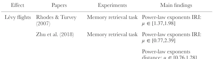
It has long been known that mental representations of concepts are also patchy (Bousfield & Sedgewick, 1944) and remarkably the distance between mental samples also follows a Lévy-flight distribution. For example, in a semantic fluency task (e.g., asking participants to name as many distinct animals as they can), the retrieved animals tend to form clusters (e.g., pets, water animals, African animals) (Troyer, Moscovitch, & Winocur, 1997). This same task has also been found to produce a Lévy-flight distribution of inter-response intervals (IRI) (Rhodes & Turvey, 2007).

2.2.1 New Experiment on Distances between Mental Samples

As we are interested in mental sampling, which can retrieve the same item multiple times, rather than destructive foraging, where an item once found is used up, we conducted a new memory retrieval experiment. Ten native English speakers (6 Female and 4 Male, and aged 19-25 years) were recruited from the SONA system of Warwick University (Coventry, UK). The task lasted about 60 minutes or until the participants typed 1024 words. Participants sat in a soundproof cubicle for this task and were paid 6 GBP for completing the experiment.

The following instructions appeared on the screen before the task began:

(31)

Participants were also told to press ENTER when they finished typing an animal name. The inter-response interval (IRI) was the duration between last ENTER pressed and the next key response.

Participants showed power-law scaling of their IRI, replicating the main finding of Rhodes and Turvey (2007) (see Figure 3A). IRIs can be considered a rough measure of the distance between mental samples, assuming that generating a sample takes a fixed amount of time, that there are unreported samples generated between each reported sample, and that the sampler has traveled further the more unreported samples that are generated. As further support, we used a standard technique from computational linguistic to measure the distances between mental samples, again finding Lévy flight distributions for these distances (see Appendix section 2.7.3)

2.3 Autocorrelations of mental samples:

1/f

noise

Separate from investigations into the distances between mental samples, a number of studies have reported that many cognitive activities contain long-range, slowly decaying autocorrelations in time. These autocorrelations tend to follow a 1/f scaling law (Kello, Brown, Ferrer-i-Cancho, Holden, Linkenkaer-Hansen, Rhodes, & Van Orden, 2010):

Hello and Welcome!

In this free association experiment, you are asked to type animal names as they come to mind. You will be shown the animal name you most recently reported on the screen and when you think of a different animal name, please type it into the computer.

We are interested in the free association of animal names, so we would like you to report what new animal you are thinking of whenever the animal you are thinking of changes.

(32)

! (2.2)

where ! is the autocorrelation function of temporal lag k. The same phenomenon is often expressed in the frequency domain:

! (2.3)

where f is frequency, ! is spectral power resulting from a Fourier analysis, and ! is considered 1/f scaling.

1/f noise is also known as pink or flicker noise, which varies in predictability intermediately between white noise (no serial correlation,

! ) and brown noise (no correlation between increments,

! ). Note that Lévy flights (i.e., randomly selecting a flight direction and then executing a flight distance that has power-law scaling as in Equation 2.1) are random walks and so produce ! noise instead of 1/f noise.

[image:32.595.111.485.637.740.2]

1/f -like autocorrelations in human cognition were first reported in time-estimation and spatial-interval-estimation tasks in which participants were asked to repeatedly estimate a pre-determined time interval of 1 second or spatial interval of 1 inch (Gilden, Thornton, & Mallon, 1995). Subsequent studies have shown 1/f scaling laws in the response times of mental rotation, lexical decision, serial visual search, and parallel visual search (Gilden, 1997), as well as the time to switch between different percepts when looking at a distal stimulus such as a Necker cube (Gao et al., 2006).

Table 1.

Empirical evidence for Lévy flights and 1/f noise in human mental samples

C(k)∼k−α

C(k)

S(f)∼f−α

S(f)

α ∈[0.5,1.5]

S(f)∼1/f0 S(f)∼1/f2

1/f2

Effect Papers Experiments Main findings Lévy flights Rhodes & Turvey

(2007) Memory retrieval task Zhu et al. (2018) Memory retrieval task

Power-law exponents distance: !μ ∈[0.76,1.28]

Power-law exponents IRI:

!

μ∈[0.77,2.39]

Power-law exponents IRI:

!

(33)

2.4 Mental Sampling Algorithms

If we have a mental representation, which is likely to be patchy for most real-world cognitive tasks, the empirical data suggest that our brain should generate samples in a manner that follows a Lévy flight distribution in distances and 1/f noise in time. Given that, we now investigate which sampling algorithms can capture both these aspects of human cognition.

We consider three possible sampling algorithms that might be employed in human cognition: Direct Sampling (DS), Random walk Metropolis (RwM), and Metropolis-coupled MCMC (! ). We define DS as independently drawing samples in accord with the posterior probability distribution. Implementing DS in the brain requires perfect representations of target distribution, be it one-dimensional or multi-dimensional. Consequently, DS is the most efficient algorithm for sampling of the three. However, DS can only be applied to relatively simple tasks. Knowing the target distribution often requires calculating intractable normalising constants that scale exponentially with the dimensionality of the hypothesis space (MacKay, 2003; Chater, Tenenbaum, & Yuille, 2006). DS has been used to explain biases in human cognition such as probability matching (Vul et al., 2014).

MCMC algorithms bypass the problem of the normalising constant by simulating a Markov chain that transitions between states according only

1/f noise Gilden et al. (1995) Time interval estimation Spatial interval estimation Gilden (1997) Mental rotation

Lexical decision Serial search Parallel search

Power spectra slope:

!

α∈[0.90,1.20]

RT power spectra slope:

!

α= 0.9

!

α= 0.7

!

α= 0.7

Power spectra slope: !α = 1

!

α= 0.7

(34)

to the ratio of the probability of hypotheses (Metropolis et al., 1953). We define RwM as a classical Metropolis-Hastings MCMC algorithm, which can be thought of as a random walker exploring the probability landscape of hypotheses, preferentially climbing the peaks of the posterior probability distribution (Metropolis et al., 1953; Hastings, 1970). The pseudo-code for RwM can be found below. Implementing RwM in the brain is relatively easy because it only needs the local information of target distribution. However, with a limited number of samples, RwM is very unlikely to reach modes in the probability distribution that are separated by large regions of low probability. This leads to biased approximations of the posterior distribution (Swendsen & Wang, 1986; Sanborn & Chater, 2016). Random walks have been used to model clustered responses in memory retrieval (Abbott, Austerweil, & Griffiths, 2012), and RwM in particular has been used to model multistable perceptions (Gershman, Vul, & Tenenbaum, 2012), the anchoring effect (Lieder et al., 2012), and various reasoning biases (Dasgupta et al., 2017; Sanborn & Chater, 2016). RwM, however, will struggle with multimodal probability distributions regardless of dimensionality.

Our third algorithm is ! , also known as parallel tempering or replica-exchange MCMC, was one of the first algorithms to successfully tackle the problem of multimodality (Geyer, 1991). ! involves running M

Markov chains in parallel, each at a different temperature: ! . In general, ! , and ! is the temperature of the interest where the target distribution is unchanged. The purpose of the heated

MC3

T₁,T₂, . . . ,T_M

1 = T₁< T₂< . . . < T_M T₁

Algorithm Random walk Metropolis

1:

2: fort=2 to Ldo

3:

4:

5:

6: end for

ifu! < Athenx! _t = x′else!x_t= x_t₋₁end if

Choose a starting point !x₁.

Sample !u ∼U[0,1], and compute !A= min{1,_ππ(x′) (xt−1)}

(35)

chains is to traverse valleys in the probability landscape and to propose moves to far-away peaks (by sampling from heated target distributions: ! ), while the colder chains make the local steps that explore the current probability peak or patch. ! decides whether to swap the states between two randomly chosen chains in every iteration (Geyer, 1991). In particular, the swapping of chain i and j is accepted or rejected according to a Metropolis rule; hence the name Metropolis-coupled MCMC.

! (2.4)

The coupling induces dependence among the chains, so each chain is no longer Markovian. The stationary distribution of the entire set of chains

is thus ! , but we only use samples from the cold chain (! ) to

approximate the posterior distribution (Geyer, 1991). Pseudo-code for !

is presented below. Note that ! can reduce to RwM when the number of parallel chains ! .

π1/T

MC3

Aswap_{= min{1,}π(xj)1/Tiπ(xi)1/Tj

π(x_i)1/Ti_π₍_x_j₎1/Tj}

M

∏

i= 1

π1/Ti _T _{= 1}

MC3 MC3

M= 1

Algorithm Metropolis-coupled Markov chain Monte Carlo

1:

2: fort=2 to Ldo

3: form=1 to Mdo

4:

5:

6:

7: end for

8:

9: Randomly select two chains i,j without repetition

10:

11:

12: end repeat

13: end for

repeat!⌊M/2⌋times

Choose a starting point !x₁.

if!u < Amthen!x_tm= x′else!x_tm= x_tm₋₁end if

Sample !u ∼U[0,1], and compute !Am= min{1,[_ππ₍_x(x_m′)

t−1)]

1/Tm_}

ifu! < Aswapthen swap(!x_ti,x_tj) end if

Draw a candidate sample !x′ ∼N(x_tm₋₁,σ)

(36)

2.5 Algorithm Selection

1

In this section, we evaluate whether the two key empirical effects of Lévy flights and 1/f autocorrelations can be produced by mental sampling algorithms.

2.5.1 Producing Lévy flights with Sampling Algorithms

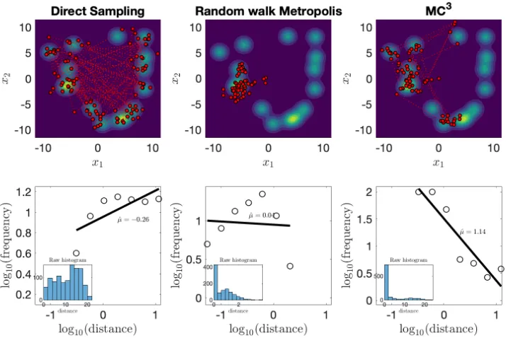
To simulate the sampling algorithms, we use a spatial representation of semantics (rather than graph structure used in semantic networks), and we justify this choice in the Appendix section 2.7.2. For generality, we first focus on simulating patchy environments without making detailed assumptions about any one participant’s semantic space. In particular, we created a series of 2D environments using ! Gaussian mixtures where the means are uniformly generated from ! for both dimensions, where ! and the covariant matrix is fixed as the identity matrix for all mixtures. This procedure will produce patchy environments (for example the top panel of Figure 2). We ran DS, RwM, and ! on this multimodal probability landscape, and the first 100 positions for each algorithm can be found in the top panel of Figure 2. The empirical flight distances were obtained by calculating the Euclidean distance between two consecutive positions of the sampler. For ! , only the positions of the cold chain (! ) were used.

N_mode= 15

[−r,r]

r = 9

MC3

T = 1

Relevant code for this section can be found at Open Science Framework: https://osf.io/

(37)

[image:37.595.117.474.77.316.2]

Figure 2. An example of searching behaviours in a 2D patchy environment. Each patch could represent a cluster of animal names (with two principal components ! ). Data points in lower panels represent binned histogram in log-log plot. Repeated simulation of samplers in different environments can be found in Figure 3. (Left Panel) Simulation result for DS. The top panel shows the trajectory of the first 100 positions (red dots). The bottom panel shows the log-log plot of flight distance distribution. The raw histogram of flight distance is also included in the bottom panel. The power-law exponent is fitted using the LBN method, which corrects for irregular spacing of points (Rhodes & Turvey, 2007). (Middle Panel) Same results from the RwM sampler. The Gaussian proposal distribution was an identity covariance matrix. (Right Panel) Same result for the ! sampler with 8 parallel chains; only the positions of the cold chain are displayed here. The Gaussian proposal distributions for all 8 chains had the same identity covariance matrix. For all three samplers considered here, only the first 1024 samples were used in order to match the length of human experiments.

Power-law distributions should produce straight lines in a log-log plot. To estimate power-law exponents of flight distance, we used the normalised logarithmic binning (LBN) method as it has higher accuracy

x₁,x₂

(38)

than other methods (Rhodes & Turvey, 2007; Viswanathan et al., 1999). In the LBN, flight distances are grouped into logarithmically-increasing sized bins and the geometric midpoints are used for plotting the data. Figure 1 (bottom) shows that only ! can reproduce the distributional property of flight distance as a Lévy flight with an estimated power-law exponent

! . Both DS (! ) and RwM (! ) produced values outside the range of power-law exponents found in human data. Indeed, RwM produces a highly non-linear log-log plot, differing in form as well as exponent from a Lévy flight. In the Appendix section 2.7.4, we support this result by showing how sampling from a low-dimensional semantic space representation of animal names with ! can produce Lévy flight exponents similar to those of produced by participants for distances.

MC3

̂

μ = 1.14 μ̂= −.26 μ̂= .04

(39)

Figure 3. (A) Animal naming task as non-destructive mental foraging (10 participants). The estimated power-law exponents for the IRIs are

! . (B) Estimated power-law exponents for flight distance

distributions for the three sampling algorithms across different patchy environments, manipulating the spatial sparsity of the Gaussian mixtures. The dashed lines show the range of power-law exponents suggested by our human data. Only ! falls in this range. (C) KL divergence of mode visitation from the true distribution for the three sampling algorithms. Red denotes RwM, black denotes ! , and blue denotes DS. The patchy environments are the same for all three algorithms. The quicker the sampler approaches zero KL divergence, the better the sampler is searching the patchy environment. The solid lines are medians of the dashed lines. (D)

Simulated standard MCMC with power-law proposal distribution. The solid

μ∈[.77,2.39]

MC3

A

[image:39.595.114.457.79.478.2]

(40)

line shows the median in estimated power-law exponent. The dashed lines show the range of human data.

Note that only one run of all three samplers in a patchy environment is shown in Figure 2. We also demonstrate the same samplers in different patchy environments with different spatial sparsities where the impact of spatial sparsity on the estimated power-law exponents was investigated (see Figure 3B). In these simulations, the same number of Gaussian mixtures was used but the range ! was varied: with higher ! , the patchy environment was more likely to be sparse. The spatial sparsity was formally defined as the mean distance between Gaussian modes. With small or moderate spatial sparsity we found a positive relationship between spatial sparsity and the estimated power-law exponents for both DS and ! (Figure 3B). In this range, only ! produced power-law exponents in the range reported in our mental foraging task unlike DS and RwM. For both local sampling algorithms (RwM and ! ), once spatial sparsity was too great, only a single mode was explored and no large jumps were made.

We then varied the values of hyperparameters and tested whether this result is robust. In particular, we sampled 4 different values respectively for temperature spacing {.5, 3, 7, 10} and the number of parallel chains {2, 4, 6, 10}, resulting in 16 combinations of hyperparameters. Intuitively, larger temperature spacing, more parallel chains, and greater step size should lead to more explorative behaviour of the sampler, and vice versa. Hence, for a certain environmental structure, ! could tune these hyperparameters to balance between explorative and exploitative searches. For searches in the semantic space of animal names, we ran ! repeatedly 10 times, and the mean of these power-law exponents was considered. 62.5% of hyperparameters reproduced Lévy flights.

We also checked whether ! really is more suitable to explore patchy mental representations than RwM. In our simulated patchy environments, which used Gaussian mixtures with identity covariance matrix, an optimal sampling algorithm should visit each mode equally often,

r r

MC3 MC3

MC3