Reconstructing Time-Dependent Dynamics
Philip Clemson, Gemma Lancaster and Aneta Stefanovska
Abstract—The usefulness of the information contained in biomedical data relies heavily on the reliability and accuracy of the methods used for its extraction. The conventional assumptions of stationarity and autonomicity break down in the case of living systems because they are thermodynamically open, and thus constantly interacting with their environments. This leads to an inherent variability and results in highly nonlinear, time-dependent dynamics. The aim of signal analysis usually is to gain insight into the behaviour of the system from which the signal originated. Here, a range of signal analysis methods is presented and applied to extract information about time-varying oscillatory modes and their interactions. Methods are discussed for the characterization of signals and their underlying non-autonomous dynamics, including time-frequency analysis, decomposition, co-herence analysis and dynamical Bayesian inference to study interactions and coupling functions. They are illustrated by being applied to cardiovascular and EEG data. The recent introduction of chronotaxic systems provides a theoretical framework within which dynamical systems can have amplitudes and frequencies which are time-varying, yet remain stable, matching well the characteristics of life. We demonstrate that, when applied in the context of chronotaxic systems, the methods presented facilitate the accurate extraction of the system dynamics over many scales of time and space.
Index Terms—Biomedical signal analysis, time-frequency anal-ysis, dynamical Bayesian inference, time-dependent dynamics, wavelet bispectrum, coupling function, phase coherence, cardio-vascular system, brain dynamics.
I. INTRODUCTION
Continuous technological advances allow the acquisition of an increasing number of biomedical signal types. These signals may arise from simple mechanical effects, such as the movement of the thorax during breathing, electrical effects, such as the synchronization of firing neurons in the brain, as measured during an electroencephalogram (EEG), optical effects, as utilised in near infra-red spectroscopy (NIRS) and laser Doppler flowmetry (LDF), or from any other measurable biological process. Improvements in the temporal resolution of these techniques allows accurate recording of the time-dependent dynamics inherent to all biomedical signals. Al-though systems on a microscopic scale may initially appear to be very complicated, there are cases when simple macroscopic behaviour may still arise from these systems [1], [2]. Decom-position of these macroscopic effects recorded by experimental signals can now be considered within already well established theoretical frameworks, based on dynamical systems which are nonlinear, non-autonomous, and far from equilibrium, as
This work was supported by the Engineering and Physical Sciences Research Council (UK) (Grant No. EP/100999X1), the EU-NEST BRACCIA Project (No. 517133), the Action Medical Research (UK) MASDA project (1963), and by the Slovenian Research Agency (Program No. P20232). The authors are with the Department of Physics, Lancaster University, Lancaster, LA1 4YB, UK. (e-mail: [email protected]).
has repeatedly been shown to be the case in living systems. Information obtained from the analysis of these signals has led to a greater understanding of fundamental physiology and is also contributing to important advances in medicine. More specifically, biological oscillations exhibiting a wide range of characteristic frequencies have been observed in biomedical data [3], spanning from very high frequencies, e.g. in EEG data [4], to very low frequencies, e.g. in cerebral hemodynamics [5], [6], microvascular blood flow [7], intracellular calcium levels [8], and individual mitochondria [9].
Although observed in many living systems [10], the im-portance of biological oscillators, and their interactions, is often overlooked, despite the fact that the extraction of their dynamics at different time scales could bring new insights and understanding of the function of living systems. In fact, these oscillations have been shown to be of great importance in many systems, such as cellular signalling [11], [12], cellular energy metabolism [13] and neural networks [14].
The coupled nonlinear oscillators approach is marked by two major milestones: the introduction of the entrainment of collective oscillators by Winfree [15] and its analysis using the phase dynamics approach of Kuramoto [16], [17]. The identification of the underlying mechanisms of some of these oscillations allows their use in the characterization of different physiological states. Observing changes in these oscillations and their interactions then yields valuable information about the underlying system, for example during epileptic seizures [18], or in skin microvascular blood flow, where changes in oscillatory behaviour have been demonstrated in pathological states with impaired microvasculature, such as hypertension [19], diabetes [20] and skin melanoma [21]. Not only do these changes in the dynamics of biological oscillators provide im-portant physiological insights, they can also be directly utilised in medicine. Potential applications include the identification of the depth of anaesthesia [22], [23], monitoring of intracranial pressure [24], and detection of impaired cerebrovascular reac-tivity after acute traumatic brain injury [25].
dynamics of an oscillatory biological system in time, with no prior assumptions. Now established as almost mandatory in biomedical signal analysis [26], time-frequency analysis methods are continually being developed for the investigation of biological systems in terms of their oscillatory components and the nature of their interactions.
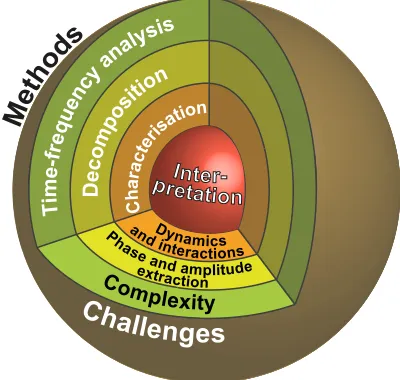
Analysis based on time-frequency methods is often like peeling an onion. Fig. 1 shows how different classes of methods can be used at each level of analysis to bring new in-formation. The initial time-frequency representation of a signal is ideal for decoding the complexity caused by combinations of nonstationary oscillations at different frequencies. These can be extracted by decomposition, which form the next class of methods. After the individual components of the signal have been separated they can be characterised by another set of methods, giving general information about the underlying sys-tem (e.g. the frequency range of the components, whether the components exchange information or are coherent). Another set of methods allow the direct physical interpretation of a modelled system from the data observed, such as whether its oscillations and interactions are stable or unstable.
Ti
m
e-fre
quen cy an
alysis
D
ecom
posit
ion
Ch
arac teris
ation
In
te
rpre tatio
n
pretation
Inter-M
et
ho
ds
Complexity
Pha
se and amplitude and interactions
extraction Dynamics
[image:2.612.314.561.56.247.2]Challenges
Fig. 1. An illustration showing the challenges related to each level of analysis and the corresponding methods used to tackle them. For biomedical time series, the challenge of the signal’s complexity must first be overcome with time-frequency analysis. This allows the identification and extraction of the phase and amplitude of individual oscillatory components using decompo-sition methods. Information from these modes can be used to characterise the dynamics of the modes and detect how they interact with each other. Finally, the properties of an explicit physical model of the dynamics provide an interpretation of the system that generated the signal.
Depending on the nature of the signal, not all of these levels of analysis may be available. For example, if the system has dominant stochastic properties, with a homogeneous ampli-tude distribution in the time-frequency representation, then it cannot be decomposed into separate oscillatory components, excluding most of the methods that would be used for the characterisation or interpretation as well. Similarly, if the system is strongly deterministic and its components could be extracted from a signal, but the signal was perhaps too short
Time Series
Wavelet Transform
Empirical Mode Decomposition Short-Time
Fourier Transform
Nonlinear Mode Decomposition
Power Bispectrum Coherence Information
and Entropy
Dynamical Bayesian Inference
[image:2.612.71.271.329.519.2]Phase Fluctuation Analysis
Fig. 2. A workflow chart of the methods discussed in this paper, organised into the levels of analysis illustrated in Fig. 1. Some methods are able to extract information directly from the original time series data. However, the methods further down the chart which are used to characterise or interpret the underlying system often depend on the outcome of time-frequency analysis and decomposition.
relative to the inherent time scales, then there is no way any meaningful interpretation can be made either.
Fig. 2 provides an overview of the methods discussed in this paper within the context of this framework. It can be seen that while some methods can be applied to the time series directly, others rely on either one or two additional steps. However, even for those that do not depend on prior analysis, there still exists a great deal of overlap between the information provided by each method. For example, if the initial time-frequency analysis shows only random noise fluctuations then the corresponding power spectrum should have a smooth continuous distribution. Similarly, the characterisation of the dynamics and interactions should match the information from the methods used to determine the actual functional relations (such as the direction of coupling between two modes).
II. RELATION TO DYNAMICAL SYSTEMS THEORY
Living systems require special treatment when their dynam-ics is analysed. This comes from the features discussed in the following sections.
A. Nonlinearity
question of the complexity of the system; a linear system can be incredibly complex or a nonlinear system can be very simple, but these fundamental rules still apply to their analysis. The effects of nonlinearity can be quite profound. Not only does it cause mathematical headaches, but it results in phenomena such ashysteresis. This describes the effect where the trajectory that a system takes from one state to another is different from the trajectory it takes in the reverse direction between the same two states, making the arrow of time important in the analysis of nonlinear systems. Nonlinearity also causes the effect ofharmonicswhich are modes that can be detected when nonlinear oscillations are analysed using methods based on linear systems.
B. Openness
The properties described above can in fact be thought of as manifestations of a single feature of living systems: the fact that they are open and exchange energy and matter with their environment. The main theories of dynamical systems typically assume that the system is closed, meaning that it is autonomous and completely described by its state in space. In contrast, living systems are open andnon-autonomous, which means they are described by both their state in space and
time. Consequently, the inclusion of time-dependent variables is vitally important in the analysis of living systems.
Note that the statistical properties of closed systems can still vary with time and the dynamics of such systems is said to
be nonstationary. Complex nonstationary dynamics in closed
systems is usually modelled by chaotic behaviour, where small perturbations in a system’s trajectory grow exponentially over time [27]. Complex dynamics that do not conform to the chaotic approach are often instead modelled by stochastic systems, where the nonstationarity arises from the influence of external random variables. Both of these approaches still fit into the framework of autonomous systems and as such time-dependent variables are traditionally not included in the analysis. However, due to the fact that living systems are not only nonstationary but non-autonomous, neither of these approaches can be applied [28].
C. Chronotaxic systems
Recently, a new class of systems has been developed which more closely captures the properties of living systems. The new model follows from the theory of self-sustained limit cycle oscillators, which have been used to describe oscillations with stable amplitude dynamics [29]. Named chronotaxic
systems, they now add to this theory by combining it with the
theory of non-autonomous systems [30] to provide a mecha-nism for stable oscillations with time-varying frequencies [31], [32]. A new framework of analysis has since been developed to detect such chronotaxic behaviour [33], [34].
To demonstrate the analytical framework discussed in this paper and its application to signals from living systems the following time series from a chronotaxic phase oscillator system are used,
x(t) = cos(αx,1t) + cos(αx,2t) + cos(αx,3t) +η1(t), (1)
where αx,i are the phases of three chronotaxic modes and
η1(t) is a 1/f noise signal. In addition, a second time series
p(t)containing the external modes which drive the x modes is defined as,
p(t) = cos(αp,1t) + cos(αp,2t) + cos(αp,3t) +η2(t), (2)
whereαp,iare the phases of the modes driving the system and
η2(t) is a separate 1/f noise signal. The chronotaxic modes
were generated using the equations,
{
˙
αp=ω0(t) ,
˙
αx=εω0(t) sin(αx−αp) +ξ(t) ,
(3)
whereεis the coupling strength from the external variablep
to the observed variablex. The functionξ(t)is white Gaussian noise with standard deviation η = √2E, where ⟨ξ(t)⟩ = 0, ⟨ξ(t)ξ(τ)⟩=δ(t−τ)E. The frequency ofαpis given as
ω0(t) =ω1[1 +Asin(ω2t)]. (4)
The modes were given the parameters [ω1= 2π,ω2= 0.016π,
A= 1] for mode 1, [ω1= 0.3π,ω2= 0.005π,A= 0.15] for
mode 2 and [ω1= 0.05π,ω2= 0.001π,A= 0.025] for mode
3. In each case the mode was made chronotaxic by setting the coupling strength|ε|= 1.5.
III. TIME-FREQUENCY ANALYSIS
Complexity is the first challenge that is encountered when dealing with biomedical signals. Not only do these signals often comprise of a mixture of oscillations at different frequen-cies, but these oscillations each have their own time-dependent dynamics. In the time domain, these oscillations cannot be easily separated. We must therefore transform the signal to
thetime-frequency domain.
A. Continuous transforms
The Short-time Fourier transform (STFT) (also known as the windowed Fourier transform), was developed as a solution to the shortcomings of the Fourier transform when dealing with nonstationary signals [35]. While the Fourier transform provides a representation of a signal in the frequency domain, the STFT transforms the data to the time-frequencydomain.
The STFT is computed by calculating the Fourier transform of a sliding window which moves over the signal. The Fourier spectrum of the window is assigned to the central point. This process is defined mathematically as
ST F T(˜ω, t) =
∫ L/2
−L/2
g(u−t)f(u)e−2πi˜lωudu, (5)
wheref(u)is a signal of length Land g(u)is a rectangular function of length l that is zero outside u, −l/2 ≤u≤l/2. The variable ω˜ is directly related to the frequencyω by ω=
˜
ω
l∆t, whilet is the time.
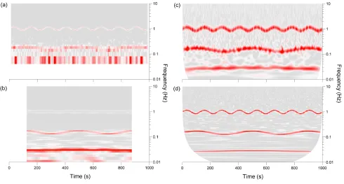
Fig. 3. Time-frequency analysis of the time series (1). STFTs of this time series are shown in (a) and (b) for a 25 s and 250 s window respectively. Continuous Morlet wavelet transforms of the same time series are shown in (c) and (d) where the central frequenciesf0= 1andf0= 5were used respectively. White spaces indicate the limit of the cone of influence where the transform is not defined.
transform. However, in Fourier transforms the frequency res-olution is proportional to the length of the data. Therefore, reducing the window size to improve time-localisation also reduces the frequency resolution and makes it more difficult to separate oscillations of different frequencies in the time-frequency domain. This limitation comes from theuncertainty
principle: one cannot determine the exact frequency of an
oscillation at an exact time. The window size also determines the lowest possible frequency that can be detected, so that the amplitude of oscillations that have frequencies below this value are merged together into the same Fourier coefficient at ω = 0. A quick fix for this problem is to use a Gaus-sian window, which provides optimal time resolution [35]. However, this still only provides the optimal resolution for the lowest observable frequencies. Higher frequencies can still be observed in smaller windows and the frequency resolution relative to the frequency of these oscillations is much better. Other solutions therefore tried to make an adaptive transform that took the frequency of the oscillation into account [36]. One such idea was to use windows of different sizes to compute each frequency in the Fourier spectrum, resulting in
the wavelet transform[37], [38].
The wavelets that form the basis of the wavelet transform are distinct from the Fourier transform in that they are defined in time as well as frequency. The continuous wavelet transform (CWT) given by
WT(s, t) = ∫ L/2
−L/2
Ψ(s, u−t)f(u)du, (6)
whereΨ(s, t)is the mother wavelet, which defines all wavelets
by being scaled according to the scalesto change its frequency distribution and time-shifted according to t. Instead of com-puting a “stand-alone transform” for each time window, the wavelet transform performs a different calculation depending on both time and frequency (or more specifically, s). This makes it possible to define an adaptive window size that is small for high frequencies and large for low frequencies. The time resolution at high frequencies is therefore no longer limited by the condition of needing a large window to detect low frequencies.
The Morlet wavelet provides a basis which is closest to the Fourier basis and is defined as [39],
Ψ(s, t) = √41 π
(
e2πiωots −e− 2πω2c
2
)
e−t
2
2s2, (7)
where s = 1/ω. The parameter ωc is the central frequency,
which determines the time-frequency resolution of the wavelet; high values (ωc > 2) give good frequency but poor time
resolution while low values (ωc < 1) give good time but
poor frequency resolution. At very small values (ωc < 0.2)
the wavelet transform becomes meaningless as the wavelets become smooth functions with no defined cycles, while at very high values relative to the length of the time series the wavelet transform has a distribution similar to the Fourier transform. A more in depth review on the technical aspects of the wavelet transform can be found in Ref. [40].
0 10 20 30 40 50 60 70 80 90 100 −5
0 5
0 10 20 30 40 50 60 70 80 90 100
0 100 200 300 400 500 600 700 800 900 1000
Amplitude
0 0.5 1 1.5 2
100 200 300 400 500 600 700 800 900 1000
0.01 0.1 1 10
TimeH(s)
FrequencyH(Hz)
(a)
(c) (d)
(b)
Fig. 4. Decomposition of the time series defined in (1). The signal reconstructed from the first 19 IMFs from EEMD is shown by the red line in (a), while the reconstruction from NMD is shown by the red line in (b). In both plots the black line corresponds to the original signal. Plots (c) and (d) show the amplitude of the modes transformed to the time-frequency domain using the Hilbert transform for EEMD and NMD respectively. The Hilbert transform generates the analytic signal of a sinusoidal oscillation, which can then be used to calculate its instantaneous frequency. This offers a direct comparison with the time-frequency analysis shown in Fig. 3.
below 0.04 Hz in (a)) or the window running over the edge of the time series. This region defines the cone of influence
for the times where oscillations of certain frequencies can be observed. However, the limitations of the time-frequency resolution are much more apparent in the STFT. In (a) the short windows allow the highest-frequency mode to be distinguished but the second mode is blurred and the third is not visible due to the low-frequency limit. In (b) the two lower-frequency modes are resolved but the highest-frequency mode fades into the background as its frequency variability cannot be tracked by the large window. In contrast, the adaptive resolution of the CWT in (c) makes it possible to resolve all 3 components simultaneously. In (d) the use of a higher central frequency improves the frequency resolution of each of the components while still allowing the variation in these frequencies to be tracked.
IV. DECOMPOSITION
The Morlet wavelet transform provides the best compromise when dealing with signals in the time-frequency domain and can be used to track time-varying oscillations. It can be interpreted in the same way as the STFT, but while this compatibility is an advantage it also means that the wavelet transform inherits the same problem of generating harmonics for nonlinear oscillations since it is still a linear method.
Further work is therefore needed to deal with the problem of decomposing and extracting individual nonlinear modes. One way to do this is by using Empirical Mode Decomposition (EMD) [41]. In this method the components are extracted by marking all of the peaks and troughs in a time series and interpolating between these two sets of points using splines. The average of these two ‘margins’ is used to define the trend of the time series, which contains dynamics relating to all but the highest-frequency component in the time series.
Subtracting this trend leaves the highest-frequency component. If there are still trends the process is repeated until
Np+Nt−Nz= 0or±1, (8)
whereNp,Nt andNz are the number of peaks, troughs and
zero-crossings respectively. Once this condition is met the extracted component is subtracted from the original time series and the method continues by attempting to extract the next highest-frequency component.
One of the problems with EMD is mode mixing, which happens when the amplitude of a mode falls to zero. The result is that the next mode replaces the one being extracted, which can result in errors if the difference in amplitudes is large. This problem has been tackled by repeating the procedure on the same time series with different iterations of additive noise and taking the average of the result, a technique known as
ensembleEMD (EEMD) [42]. However, the iterative nature of
EMD is still susceptible to error propagation, causing small errors in the extraction of high-frequency components to affect the extraction of the lower-frequency components.
An alternative to EMD is to use information from the time-frequency domain to decompose the time series. Specifically, identifying all of the harmonics of a nonlinear mode in the time-frequency domain makes it possible to separate and re-construct this mode in the time domain. This can be done in the wavelet transform by making use of the time-dependent phase information of the oscillations, which is given by ϕ(s, t) =
arg[Wt(s, t)]. Assuming the waveform of the oscillation keeps
the same shape, the phases of harmonics will share the same dynamics. This means that two harmonics at scaless1ands2
will have the relationϕ(s1, t) = (s1/s2)ϕ(s2, t).
[image:5.612.51.563.57.239.2]noise fluctuations in the fundamental mode, the real dynamics of the mode can be more easily separated from the noise this way. The most recent method, Nonlinear Mode Decomposition (NMD), uses information from the harmonics to improve the extraction of the mode as a whole [44]. Specifically, the method is based on ridge extraction where the highest peak over a defined frequency range in the wavelet transform is traced over time. This line can then be used to extract the oscillation at the defined times and frequencies. The algorithm then looks at the phase and amplitude variations of several oscillations together in order to distinguish harmonics (which share the same variations) from genuine independent modes.
Fig. 4 compares EEMD with NMD in the analysis of the example time series x(t). While the oscillatory modes are observable in both decompositions, NMD is more selective and does not extract modes relating to the 1/f noise. The continuous noise distribution means that the modes calculated using EMD suffer from mixing, which means it is not possible to isolate the three main oscillatory modes. Instead, most of the EMD modes are associated with high-frequency components which try to fit the original time series as closely as possible and as such do not have much physical meaning.
V. CHARACTERISATION
After transforming a signal to the time-frequency domain and/or extracting its oscillatory modes, the next step is to use this representation to characterise the dynamics of the system. This means connecting what is seen in the signal with properties that can be related to a physical system.
A. Power
The power spectrum of a time series is defined in the fre-quency domain as the integral of the square of the amplitude. For the Fourier transform this is a straightforward process since the frequency scale is linear, causing the square of the Fourier transform to be directly proportional to the power spectrum. Similarly, the wavelet power spectrum can be found using
PW(ω′, t) =
∫ ω′+dω 2
ω′−dω
2
|WT(ω, t)|2dω. (9)
However, in the case of the wavelet transform the frequency scale is logarithmic, which means that the components at higher frequencies correspond to larger frequency intervals. Obtaining the power spectrum from the Morlet wavelet trans-form is also not as simple because the transtrans-form is continuous. This means that although the wavelet amplitude is analogous to the Fourier amplitude, for finite data the integration of the squared amplitude to find the power is always an estimate (a continuous curve cannot be integrated discretely).
Taking the average ofPW in time provides a good starting
point in the analysis of any time series data. Specifically, it is used to identify the frequency range of the main oscillatory components. Once this is known, the variation in the power of each individual component over time can be found using one of the two methods shown in Fig. 5(b). The first method involves summing over the wavelet transform in the frequency
intervals defined in the time-averaged power spectrum for each point in time (black line). The second method is to instead follow the peak in the power spectrum for the given frequency interval in time (grey line), which is known as ridge extraction [45]. As can be seen, the two methods show similar fluctuations caused by the noise in the system although the second method is less susceptible to these variations.
B. Bispectrum
The bispectrum is a frequency-frequency domain method that arises from high-order statistics [46]. Specifically, the bispectrum is a third order statistic, in the same sense that the skewness of a data series is of the third order, which comes after the mean (first order) and variance (second order) [47]. In this case the bispectrum is the next order measure after the frequency domain spectrum of a time series.
The bispectrum provides information about the quadratic properties of the time series, which makes it ideal for in-vestigating nonlinear couplings between oscillations. However, the frequency-frequency domain is still unable to track time-variability. Therefore, similar to the need for time-frequency analysis, a need for time-frequency-frequency analysis lead to a proposal of wavelet-based bispectral analysis [48]. The wavelet bispectrum is given by,
BW(s1, s2) =
∫
L
WT(s1, t)WT(s2, t)WT∗(s3, t)dt, (10)
where s3 = 1/(s11 + s12). It is also possible to define
an instantaneous bispectrum with amplitude A(s1, s2, t) =
|WT(s1, t)WT(s2, t)WT∗(s3, t)| and phase ϕ(s1, s2, t) =
ϕ(s1, t) +ϕ(s2, t)−ϕ(s3, t).
Couplings between two oscillations at s1 and s2 can be
identified by peaks in the amplitude of the bispectrum or by observing the dynamics of the phaseϕ(s1, s2, t), where if the
phase is constant a coupling exists [48]. In the case of the amplitude though, the value is also dependent on the amplitude of the oscillations in the wavelet transform. To remove this effect a normalised version can be defined as
b(s1, s2) = |
BW(s1, s2)|
√∫
L|WT(s1, t)WT(s2, t)|
2dt∫
L|WT(s3, t)|
2dt
,
(11) whereb(s1, s2)is known as the bicoherence and takes values
between 0 and 1. However, even with this normalisation it is important to note that the bispectrum / bicoherence will still be non-zero for Gaussian white noise. These random peaks are biased towards lower frequencies, with a chi-squared distribution [49], [50], [51].
An additional complication comes from dealing with the scales3, which causes the bispectrum to become meaningless
as both f1 = 1/s1 and f2 = 1/s2 approach the Nyquist
frequencyfs/2. This is becausef3starts to take amplitude and
phase information at frequencies which are outside the observ-able range. Couplings at the highest frequencies are therefore not detectable, meaning an ‘effective’ Nyquist frequency for the bispectrum is defined as the line from f1 = fs/4,
f2=fs/4 tof1=fs/2,f2= 0 (and vice versa for whenf1
0.01 0.1 1 0
0.005 0.01 0.015 0.02 0.025 0.03
Frequency (Hz)
Time−averaged power
0 1 2
0 1 2
Normalised power
0 100 200 300 400 500 600 700 800 900 1000
0 1 2
Time (s)
Sum over interval Peak over interval (a)
Mode 1
Mode 2
Mode 3 Mode 3 Mode 2 Mode 1
[image:7.612.95.522.57.189.2](b)
Fig. 5. Wavelet power spectrum of the time series (1). The time-averaged power spectrum is shown in (a), where the frequency ranges of the three modes are defined using the minima at each side of the peak (yellow shaded regions). In (b) the power of the three modes is traced in time using the sum and peak methods. The power is normalised by dividing by the sum or peak of the time-averaged spectrum respectively.
Fig. 6. Wavelet bispectrum analysis for the time seriesx(t)andp(t). The bicoherence for the various combinations of the cross-bispectrum are shown in (a), where without the time axis it is difficult to distinguish the amplitude due to noise fluctuations from the amplitude contributions of genuine couplings. In (b) and (c) the bispectral amplitude and phase are shown for the points marked in (a) which correspond to the coupled frequency pair (1 Hz, 1 Hz) and unrelated frequency pair (0.6 Hz, 1.4 Hz). While the amplitude is higher for the coupled pair, the coupling is also indicated by the fact that the phase does not grow over time.
One other disadvantage is that wherever the difference in the frequencies of a pair of oscillations is large, the adaptive frequency resolution of the wavelet transform means that the combined frequency fHIGH + fLOW ≈ fHIGH, making these couplings undetectable. On the other hand, the logarithmic frequency scale of the wavelet transform means that couplings between pairs of low frequencies can be identified.
The same method can also be used to detect couplings between components from different time series. The cross-bispectrum can be defined in several ways [48], [52], [53] using different combinations of the three wavelet components in (10), i.e.
B122W (s1, s2) =
∫
L
W1(s1, n)W2(s2, n)W2∗(s3, n)dn, (12)
where W1 and W2 are the wavelet transforms of the
cor-responding time series. The wavelet cross-bicoherence can similarly be defined as [54]:
bW122(s1, s2) = |
BW122(s1, s2)|
√∫
L|W2(s1, t)W2(s2, t)|
2dt∫
L|W1(s3, t)|
2dt
.
(13) By comparing the cross-bispectra from different combinations it is also possible to deduce some information about the direction of coupling between the oscillations in two separate time series.
Fig. 6 shows the bispectral analysis of the time seriesx(t)
[image:7.612.52.560.246.490.2]Fig. 7. Wavelet phase coherence between the time seriesx(t)andp(t). In (a) significant phase coherence is shown when the coherence (black line) is greater than the 95th percentile of 100 pairs of IAAFT surrogates (grey line). The windowed phase coherence is shown in (b), which reveals the time-variability of the modes but at the cost of losing information about lower frequencies.
frequencies. These interactions appear due to the 1/f noise present in the time series, which makes the time-averaged bispectrum difficult to interpret. However, when the phase of a coupled frequency pair is compared in time with that of two unrelated frequencies it is clear that the phase corresponding to the coupled frequencies is locked and stays close to its original value.
C. Coherence
Waves can be coherent in space and oscillations can be coherent in time. Generally, coherence in time describes all properties of correlation between physical quantities of a single oscillation, or between several oscillations. Like power, bispectral amplitude and phase, coherence is defined for specific frequencies. If at a certain frequency the changes in amplitude and phase of an oscillatory component are the same for the same oscillation observed in different time series, then they are said to be coherent at that frequency. While this is the general definition of coherence, it is also possible to define separately amplitude and phase coherence, which consider only matching amplitude or phase dynamics of the components respectively.
A phenomenon related to coherence is synchronization. However, while oscillations can be coherent without direct coupling, synchronization is a property of the underlying system which results from a coupling between two oscillations. This phenomena is not as trivial as one might expect, with multiple ways to both define and detect synchronization [55]. Specifically, oscillators can be phase synchronized, phase and amplitude synchronized or Lyapunov synchronized (also known as generalised synchronization) and also have n : m
relations where there arencycles of one oscillator inmcycles of the other. Phase coherent oscillations can result in 1:1 phase synchronization.
In the case of biomedical signals, measures of phase synchronization are often used as a simple way to observe interactions between two oscillations. Methods such as the
phase synchronization index typically rely on the detection of phase locking, where the phase shift between two oscillations remains constant [56]. However, if only 1:1 synchronization between two signals is of interest then it is more straightfor-ward to consider the phase coherence instead, which is defined as [57],
Π(s) = 1 N
N ∑
n=1
ei(ϕ1(s,tn)−ϕ2(s,tn))
, (14)
whereϕ1(s, tn)−ϕ2(s, tn)is the phase difference between the
oscillatory components of the same frequency from two signals at timetn. If the oscillations remain phase locked for all time
(i.e. the oscillations are coherent) thenΠ(s) = 1, whereas if
Π(s) = 0 there is no tendency to preserve a particular phase difference. A more general definition is also given by [58],
Π =
{[
1 2
N ∑
n=1
w1(tn)w2∗(tn) ] [
1 2
N ∑
n=1
w1(tn)∗w2(tn) ]}1/2
(15) wherewi(t)represents any time-frequency representation with
complex values corresponding to the analytic signals of the oscillations. In this paperΠwill represent the phase coherence of the power-normalised wavelet transform, which is identical to the first definition shown above.
The phase coherence can be calculated systematically for all wavelet scalessto provide a graph of coherence vs. frequency [59], [60], [61]. However, even in the phase coherence of two noise signals there is some level of coherence. This means that the coherence rarely approaches 0 and significant coherence is usually close to 1. Additionally, this baseline coherence is not constant for all scales but increases when moving lower in frequency to the point where at the lowest observable frequenciesΠ(s)≈1 even if the dynamics is unrelated.
This bias towards lower frequencies can be accounted for by usingsurrogatesof the signals [62], [63]. These are designed to preserve all of the properties of the original signals apart from the property relating to the hypothesis that is being tested. In the case of phase coherence, the null hypothesis is that the phases in the signals are independent for all frequencies, which means that it is the time-phase information that needs to be randomised in the surrogates. In this case, iterative amplitude adjusted Fourier transform (IAAFT) surrogates fit this null hypothesis [64]. The phase coherence between these surrogates at each frequency can then be used as a baseline above which the coherence is said to be significant.
a significant reduction in the part of the time series that is observable at low frequencies. Finally, to observe significant coherence at least 5 cycles need to be observed [36], which further raises the low-frequency limit of the analysis.
Fig. 7 shows the phase coherence of the example time series
x(t)andp(t). It can be seen that the coherence is only greater than the surrogate level at the frequencies corresponding to the common oscillatory modes. Note however that the surrogate level is inversely proportional to the frequency, which means it is more difficult to detect significant coherence in low-frequency oscillations. The windowed wavelet phase coher-ence also reveals the shared time-variability of these modes.
D. Information and entropy
Wavelets are not the only available tool for the analysis of interactions in complex systems. Another way to detect couplings is by using statistics based on information theory, such as transfer entropy [65] and Granger causality [66], [67]. In the latter case, a coupling is said to exist if one system gives information about the state of the other system at some point in the future [48], [62], [68], [69]. Starting with the probability distributions of the two time series,p(x1(t))andp(x2(t)), the
Shannon entropy for each can be defined as
H(xi) =− ∑
p(xi) logp(xi), (16)
which gives a measure of the uncertainty or ‘randomness’ in
xi. Thejoint entropy can also be defined as
H(xi, xj) =− ∑ ∑
p(xi, xj) logp(xi, xj), (17)
where p(xi, xj) is the 2-dimensional joint probability
distri-bution. The amount of common information contained in xi
andxj, which is analogous to the inverse of the joint entropy,
is given by the mutual information:
I(xi;xj) =H(xi) +H(xj)−H(xi, xj). (18)
Finally, the conditional entropy is defined as
H(xi|xj) =− ∑ ∑
p(xi, xj) logp(xj|xi), (19)
where p(xj|xi) is the probability distribution for xj if the
value for xi is given. The dependence between xi and xj
without the possible influence of another variablex3 can then
be defined using the conditionalmutual information (CMI),
I(x1;x2|x3) =H(x1|x3) +H(x2|x3)−H(x1, x2|x3). (20)
Consider now two time seriesx(t)andy(t). The information flow from x to y is given by I(x;yd|y), where yd is the
delayed time series y(t+τ) with l∆t = τ. This quantity excludes information from both the history of y(t) on itself and the common history of x(t) and y(t) [48]. Similarly, the information flow from y to x is given by I(x;yd|y).
Therefore, the strength of coupling from one time series to another should be indicated in the amount of information flow in the corresponding direction.
In reality, there is always going to be some baseline mutual information contained within even two completely unrelated time series. This is why the method requires the use of
0 0.02 0.04 0.06 0.08
I
(
x
;
pd
|
p
)
0 200 400 600 800 1000
0 0.02 0.04 0.06 0.08
Time (s)
I
(
p
;
xd
|
x
)
(a)
(b)
Fig. 8. Information analysis of the time seriesx(t)andp(t). The solid black lines show the average CMI calculated for delays ranging from 0.05 s to 5 s. The grey lines show the 75th percentiles of the CMI calculated between 100 pairs of IAAFT surrogates. The information transfer in the directionp→xis shown in (a), while (b) shows the information transfer in the directionx→p.
surrogate data to determine whether there is a significant
amount of information being transferred either fromx1→x2
orx2→x1. It is also dependent on estimates of the probability
distributions of the time series, which require careful consid-eration. However, the main advantage of this approach is that it is not restricted by frequencies; the CMI gives a measure of the information transfer between two arbitrary sets of data, rather than being localised in any one domain. It is also worth noting that Granger causality can be calculated using other methods that do not rely on CMI [70].
An advantage of information and entropy based measures is that they are dimensionless, meaning that they can be applied to any type of signal. In particular, they can be applied both to the raw signal but also to the extracted phases of the oscillations in order to determine specific phase-phase interactions [48], [68].
Fig. 8 shows the CMI of the time series defined in (1) and (2). It can be seen that there is much more significant information transfer above the surrogate level for I(x;pd|p)
as opposed to I(p;xd|x), which suggests a coupling from
the modes in p(t) to the modes in x(t). However, it is also worth noting the times when there appears to be no transer of information. This can be explained by the fact that the chronotaxic modes are very close to being phase synchronized with the driving modes in p. When they do become fully synchronized there is no transfer of information, which means that even if there is a coupling it is not possible to detect one.
VI. INTERPRETATION
Fig. 9. Dynamical Bayesian inference analysis of the phases extracted using NMD from the time seriesx(t)andp(t). Plots (a), (b) and (c) show the coupling functions for the pairs of phases extracted from each mode. The inferred value ofω0(t)is shown in (d), (f) and (h) by the solid black line, while the dotted line is the actual value. Plots (e), (g) and (i) show the direction of coupling calculated by taking the ratio of the amplitudes for the terms dependent on the other phase for each coupling function.D >0for a coupling in the directionx→pandD <0for a coupling in the directionp→x. The model parameters were inferred using a 20 s moving window with 50% overlap for mode 1, a 150 s window with 75% overlap for mode 2 and a 500 s window with 90% overlap for mode 3. In each case the propagation constant had the valuep= 0.2
information it is necessary to infer the properties of a physical model of the system based on the observed dynamics.
A. Phase oscillator model
Living systems are characterised by a multitude of oscilla-tions over a broad range of timescales. However, the real com-plexity arises from the interactions between these oscillations, and there have been many attempts to model this accurately [3]. The simplest models of coupled oscillators focus purely on the changes that occur in an oscillator’s phase over time and neglect any amplitude variations. This simplification is justified in models of the heart (or similar oscillators with all-or-nothing responses), because it is only changes in the timing of the periodic features that carry significance. Even when a system does vary in amplitude, many oscillators can still remain close to an attracting limit cycle, which again causes these variations to be negligible.
An example of a phase oscillator model is given bydϕ/dt= ω, which describes a phase increasing at a rate of ω, which is the natural frequency of the oscillator. A model of two interacting oscillators is given by
dϕ1
dt =ω1+F1(ϕ1, ϕ2), (21)
dϕ2
dt =ω2+F2(ϕ1, ϕ2),
whereF1(ϕ1, ϕ2)andF2(ϕ1, ϕ2)arecoupling functionswhich
allow the dynamics of one oscillator to be dependent on the other. Such coupling functions are expected to be periodic on
the phasesϕ1andϕ2, which means that they can be modelled
by a Fourier series [71],
F1,2(ϕ1, ϕ2) =
∑
l,m [
a1,2(l,m)cos(mϕ1+lϕ2) (22)
+b1,2(l,m)sin(lϕ1+mϕ2)
]
, (23)
wherea1,2(l,m)andb1,2(l,m)are the parameters which describe
the function. By inferring these parameters from the observed dynamics of the system it is possible to gain an in-depth understanding of the oscillations, such as whether they exhibit synchronization, or how they respond to perturbations.
B. Dynamical Bayesian inference
A problem with the model shown above is that the pa-rameters are stationary. This makes it more difficult for this model to reveal information about the coupling functions in non-autonomous systems, which are expected to be time-dependent. However, there is no straightforward way to apply a moving time window because windowing means that a smaller data series goes into the algorithm used to estimate of the couplings, increasing the uncertainty.
The Bayesian theorem offers a solution to this windowing problem. When applied to inverse problems where one would like to infer parameters related to the generation of a data set [72], [73], [74], [75], [76] it is known asdynamical Bayesian
inference. The theorem is summarised in
P(M|X) = P(X |M)Ppr(M)
whereP(X |M)is the conditional probability of observing the dataX given the hypothesised parametersM.Ppr(M)is the probability of Mbefore observing the dataX and
P(X) =
∫
P(X |M)Ppr(M)dM (25)
is the marginal probability of X. P(M|X) is known as the
posterior probability – the probability that the hypothesised
parameters are correct given X and the prior probability
Ppr(M).
The most likely combination of values for the parameters for a single window of data is inferred by locating the stationary point in the negative-log likelihood function, known as maximum likelihood estimation. In this case the likelihood function is specified for the phases of two systems [75] defined by the following stochastic differential equations,
dϕ1,2
dt =ω1,2+F1,2(ϕ1,2) +G1,2(ϕ1, ϕ2) +ξ1,2(t), (26)
where F1,2(ϕ1,2) and G1,2(ϕ1, ϕ2) are coupling functions
which, as in the previous methods, are modelled using a Fourier basis. The parameters ck for this basis are eventually
inferred in a covariance matrix denoted Ξ. By making use of Bayes’ theorem, the posterior covariance matrix for the previ-ous window can exploit information from the prior covariance matrix Ξprior for the current window. Hence, information is allowed to propagate between windows, enabling the inferred parameters to become more accurate with time [75].
However, the inference only improves if the parameters do not vary in time. To account for changes in the values of the parameters, the prior can take the form of a convolution between the posterior of the previous window and a diffusion matrix which describes the change in ck [75]. The standard
deviation corresponding to the diffusion of the parameters is assumed to be a known fraction of the parameters themselves,
σk = pck, where p is known as the propagation constant.
This modification allows the method to track the change in the couplings over time.
A tutorial for the implementation of this Bayesian-based approach is provided in [77], which includes a Matlab toolbox. Fig. 9 shows the method applied to the extracted phases of the example time seriesx(t)andp(t). The coupling functions for the modes in x(t)have a much higher amplitude than the modes in p(t), which suggests a strong coupling term such as the one present in the chronotaxic modes. The method also reconstructs the time-variability ofω0 for the first mode.
However, for the other modes the frequency variation is not traced as well because the window sizes are much larger in order to cover enough cycles of the low-frequency oscillations. Despite this, in all cases the method correctly identifies a coupling in the direction from the modes in p(t) to those in
x(t).
C. Phase fluctuation analysis
Let us now return to chronotaxic systems, which were introduced in Sec. II-C. They are non-autonomous systems and have stable dynamics relative to a time-dependent point
−2 −1 0 1 2
∆αx
1 2 3 4 5 6
log(F)
−1 −0.5 0 0.5 1
∆αx
2 3 4 5
log(F)
0 200 400 600 800 1000 −1
−0.5 0 0.5 1
Time (s)
∆αx
5 6 7 8 9
2 3 4 5 6
log(n) log(F)
(c) (b) (a)
α= 0.97
α= 0.90
α= 1.57
(e) (d)
(f)
Mode 1
[image:11.612.317.558.59.276.2]Mode 3 Mode 2
Fig. 10. Phase fluctuation analysis analysis of the modes in the time series x(t). Estimates of the phaseαx for mode were obtained from the wavelet transform using ridge extraction andωc = 0.5. Estimates of the phaseαu were found in the same way but using ωc = 2 and integrating over the smoothed instantaneous frequency. Plots (a), (b) and (c) show the detrended difference between the two phases for each mode. Plots (d), (e) and (f) show the detrended fluctuation analysis of∆αx (solid black lines). Linear least squares fits (red lines) were used to estimate the values ofαin each case.
attractor [31]. This property determines how the system re-sponds to perturbations, whether resisting them or allowing them to dictate their dynamics. However, despite this strong dichotomy, the actual effects are not obvious and hidden even in the time-frequency domain. Another approach is therefore needed.
The easiest way to determine whether a system is chrono-taxic or not is to observe its fluctuations relative to its unperturbed trajectory. If the original distribution of the per-turbations is known, then the stability of the system relative to the unperturbed trajectory (which by definition follows the time-dependent point attractor in a chronotaxic system) can be determined from how these fluctuations grow or decay over time. For example, take the non-chronotaxic phase oscillator
dαx
dt =ω0(t) +η(t), (27)
whereω0(t) is the time-dependent natural frequency and the
observed phase αx is perturbed by noise fluctuations η(t).
Integrating we find
αx= ∫
ω0(t)dt+
∫
η(t)dt. (28)
Assuming thatω0(t)>0andη(t)is an uncorrelated Gaussian
process, this means that the dynamics ofαx will consist of a
for a chronotaxic phase oscillator, e.g.
dαp
dt =ω0(t), (29)
dαx
dt =εω0(t) sin(αp−αx) +η(t),
whereαp is an external phase and |ε|>0. Here the stability
provided by the point attractor causes each noise perturbation to decay over time, preventing η(t) from being integrated over to the same extent. The perturbations still do not decay instantly as the system takes time to return to the point attractor, meaning that some integration of the noise still takes place. However, the size of the observed perturbations over longer timescales is greatly reduced, causing a change in the overall distribution from that expected for Brownian motion.2 The phaseαxof the observed system can be estimated using
the decomposition methods mentioned in the previous section. However, further work is needed to obtain the unperturbed phaseαu
x. In particular, it is difficult to separate the dynamics
corresponding toαu
xfrom the effect of the noise perturbations
η(t). This task is simplified by assuming that the dynamics of αu
xis confined to timescales larger than a single cycle and
that the noise is either weak or comparable in magnitude. With these assumptions, an estimate of αu
x can be found
by filtering out high-frequency components of αx. However,
such a filter should not smooth over the dynamics of αu
x.
An optimal way of removing these high-frequency noise fluctuations without affecting the unperturbed dynamics is to instead smooth over the frequency extracted from the wavelet transform [33]. This provides the estimated angular velocity
˙
αux, which can in turn be integrated over time to giveαux.
Given the estimates ofαxandαux, the next step is to analyse
∆αx=αx−αux to find the distribution of fluctuations in the
system relative to the unperturbed trajectory.
In order to quantify the distribution of fluctuations, de-trended fluctuation analysis (DFA) can be performed on∆αx
[78], [79]. This method provides an estimate of the fractal self-similarity of fluctuations at different timescales. The scaling of these fluctuations is determined by the self-similarity param-eter α, where fluctuations at timescales equal to t/a can be made similar to those at the larger timescaletby multiplying with the factor aα.
In order to calculate αthe time series∆αxis integrated in
time and divided into non-overlapping sections of length n. For each section the local trend is removed by subtracting a fitted polynomial – usually a first order linear fit [78], [79]. The root mean square fluctuation for the scale equal to n is then given by
F(n) =
v u u
t1
N
N ∑
i=1
Yn(ti)2, (30)
where Y(t) is the integrated and detrended time series and
N is its length. The fluctuation amplitude F(n) follows a
2Note that this assumes the noise does not cause phase slips inα x. This would cause perturbations over large timescales (i.e. greater than one cycle) to not decay even if the system was chronotaxic. In these cases another approach should be used instead [33].
scaling law if the time series is fractal. By plottinglogF(n)
againstlogn, the value ofαis simply the gradient of the line. For completely uncorrelated white Gaussian noise (the noise assumed to perturb the system) the parameter for α has a value of 0.5, while integrated white Gaussian noise (expected in non-chronotaxic systems) returns a value of 1.5.
When α < 1.5 this therefore suggests that there is some resistance to perturbations (chronotaxicity) which prevents their integration over larger timescales. The actual value is typically dependent on the gradient of the coupling function relative toαp−αx. If the gradient close to the point attractor
is very steep then the system returns to the attractor more quickly after being perturbed and less integration of the noise occurs, resulting in smaller values ofα.
Fig. 10 shows the phase fluctuation analysis for the extracted phases of the modes in the time seriesx(t). The method finds
α <1 for the first two modes, which suggests that they are chronotaxic. However, the method identifies the third mode as being non-chronotaxic since α ≈ 1.5. This is due to the fact that not enough cycles of the oscillation are observed to reliably determine whether the mode is chronotaxic or not.
VII. APPLICATIONS
To demonstrate how the described analytical framework can be used in practice, the methods from the previous sections are now applied to real biomedical signals.
A. Skin microvascular flow evaluated by Laser Doppler flowmetry (LDF)
LDF is a technique applied to measure blood flow in the microvasculature. It involves shining laser light into the mi-crovascular bed, that includes capillaries and small arterioles, and measuring the Doppler shift in the light caused by the movement of the blood. This movement is influenced by a wide range of oscillations of different frequencies ranging from 0.005 Hz to 2 Hz, originating from both systemic and local processes [7], [3], [79]. As each of these oscillations is also time-varying, the result is a very complex signal.
Fig. 11 shows the time-frequency analysis of an LDF signal. The strong cardiac oscillation is easily recognised in the Fourier transform. However, there is also power at low frequencies which appear as a continuous noise-like distri-bution. The wavelet transform reveals these low-frequency fluctuations to be highly nonstationary oscillations, relating to myogenic, neurogenic and endothelial activity [7]. Without time-frequency techniques, such oscillations can often elude discovery or be discounted as noise [26].
Fig. 11. Analysis of an LDF signal measured from the left arm for 40 minutes. In the time domain (top) the cardiac oscillation is clearly seen, with∼1s pulses. A Fourier transform (bottom left) provides a representation of the signal in the frequency domain, which also shows the mode with the largest power to be at the cardiac frequency∼1Hz with its harmonics at∼2Hz and∼3Hz. There is also power at lower frequencies but this appears only as a continuous, noise-like spectrum with no identifiable modes. In the wavelet transform (bottom right) the power at low-frequencies is revealed to be due to nonstationary oscillations whose frequencies and amplitudes vary in time.
of recordings is limited by the fact that subjects must remain motionless throughout as movement artefacts strongly affect the low-frequency components of the signal [80]. But even when only the power of the oscillations is considered, without attempting to consider their coupling, the insights obtained can be of diagnostic and prognostic use, as shown in a recent study of blood flow in melanoma [21].
On larger scales, the dynamics of the cardiovascular sys-tem is no less complex. In particular, the cardiorespiratory interaction has been shown to exhibit time-dependent coupling functions which cause changes in the synchronization between the heart and lungs [75]. This interaction is primarily defined by the phase relationship between the two systems, which means that it is maintained even when the variations in the heart rate or respiration amplitude are small. Using bispectral analysis this coupling has been shown to propagate to the microcirculation [81].
B. Dynamics of brain waves and their interaction in anesthe-sia and awake states
The neuronal activity in the brain has long been charac-terised by existence of brain waves [4] and we will briefly illustrate how interactions between brain waves can be ex-tracted from an EEG signal. The signal was recorded in the BRACCIA project with electrodes attached to the forehead of a patient under anaesthesia [23]. The traditional waves, δ
(0.8–4 Hz),θ(4–7.5 Hz),α(7.5–14 Hz),β (14–22 Hz) andγ
(22–100 Hz) were studied. Lower frequency oscillations have also been identified [4], [3], but will not be discussed here. The results of bispectral analysis and dynamical Bayesian inference are summarised in Fig. 12.
When analysed using the wavelet bispectrum, the noise in the signal makes it difficult to interpret the interactions from its amplitude alone. However, the phase of the bispectrum for each frequency coupling shows different rates of change, related to the coupling strength between the brain waves. After extracting the phases for each brain wave, Bayesian inference reveals the coupling functions between the oscillations, as well as the magnitude of these couplings. By observing the ratios between the grey and black lines it is possible to infer the direction of coupling between the brain waves. It can be seen that the other waves drive theγ wave, which is also observed in the form of theFγ coupling functions. While this provides
clear evidence of functional interactions between pairs of brain waves, the same techniques have also been used to show the existence of triplet interactions [82].
VIII. DISCUSSION
Biomedical signals, arising from nonlinear, time-dependent living systems, provide an opportunity to monitor the underly-ing dynamics of the observed system. The time-variability of biomedical data necessitates the application of time-frequency analysis methods in the first instance. If identified as a stochastic process, the signal may be further characterised using statistical methods. If the signal is found to contain distinct oscillatory modes, these may then be extracted and separated using the techniques presented here. The interactions between these modes can be then investigated to provide yet another layer of information about the dynamics of the system. Living systems appear to possess underlying preferred amplitudes and frequencies to which the system will return when external influences are removed. To bridge the gap between dynamical systems theory and this apparent stabil-ity, a new class of nonautonomous system was introduced, known as chronotaxic systems [31], [32]. This led to the development of methods for the detection of chronotaxicity and their application to real data [33], [34]. This provides a framework in which experimentally observed fluctuations, which may previously have been regarded as noise, or arising from chaotic dynamics, may actually be considered as systems with underlying elements of determinism.
Fig. 12. (a-c) Bispectral and (d,e) dynamical Bayesian inference analysis of an EEG signal. The signal was measured for 20 minutes from the forehead of a subject in anæsthesia. The phases for theδ,θ,α,βandγwaves were extracted using NMD. The plot in (a) shows the bicoherence of the raw EEG signal, while (b) and (c) show the instantaneous bicoherence and phase of the bispectrum respectively for the pairs of brain waves. In (d) the coupling functions for the different pairs of extracted phases are shown (couplings between adjacent bands are not shown due to frequency spillage from imperfect filtering). On the right in (e) are the magnitude of the coupling functions for each point in time, providing an indication of the direction of coupling between the phases. The model parameters were inferred using a 20 s moving window with no overlap and with the propagation constantp= 0.2.
their origins. Also important when extracting modes from a time-frequency representation is the frequency variation. If this variation is too fast, or more than one mode is present, it may be difficult to reliably extract a single mode. The frequency resolution in the wavelet transform may be changed to better resolve frequency components, but this comes at the expense of time resolution and may still be insufficient.
In some living systems, only the phase dynamics is consid-ered. For example, in the heart only the changes in beat rate can be directly measured with ease, while the cardiac output (the “amplitude” of the heart) is very difficult to quantify by noninvasive techniques. Whilst some of the presented methods rely on the fact that amplitude variations may be negligible, this is not always a valid assumption. Again using chronotaxic systems as an example, the current inverse approach methods for the detection of chronotaxicity only take into account phase dynamics. However, it is known that in many living systems, both phase and amplitude dynamics are important, as are the interactions between them. In particular, the brain is characterised by both spatial and temporal dynamics [83], [84]. Thus, further work is required to develop methods which are
applicable in all these scenarios, although some have already been proposed [85]. It is clear that to gain as much information as possible from biomedical signals, the optimal solution is to combine different methods according to the information required, as demonstrated here.
IX. CONCLUSION
[image:14.612.52.565.56.409.2]