Numerical and experimental investigation of a vortical flow inducing jet pump

Conference on Modelling Fluid Flow (CMFF’18) The 17th _{International Conference on Fluid Flow Technologies} Budapest, Hungary, September 4-7, 2018

N

UMERICAL AND

E

XPERIMENTAL

I

NVESTIGATION OF A

V

ORTICAL

F

LOW

-I

NDUCING

J

ET

P

UMP

Andrew MORRALL

_{, M. Sergio CAMPOBASSO}

_{, Stephen QUAYLE}

1 _{Corresponding Author. Department of Engineering, Faculty of Science and Technology, Lancaster University. Lancaster, United} Kingdom, E-mail: [email protected]

2 _{Department of Engineering, Faculty of Science and Technology, Lancaster University. E-mail: [email protected]} 3 _{Department of Engineering, Faculty of Science and Technology, Lancaster University. E-mail: [email protected]}

ABSTRACT

Experimental analyses and CFD simulations are performed on a vortical flow-inducing jet pump. The device is a multi-nozzle annular jet pump, in which a high-pressure fluid is injected into a bore through circumferentially distributed nozzles. The nozzles are angled axially and radially so that the injected primary fluid produces both suction and a vortical flow pattern. Analysis of the pump is considered as single phase, using compressed air to pump atmospheric air. Experiments are carried out on two jet pump designs, working at different conditions with results used to validate CFD simulations. CFD turbulence model analyses is used to determine the optimal numerical method, with hybrid turbulence models shown to be effective in predicting the pressure produced by the swirling flow phenomena. Suction pressure induced by the jets is shown to be highly dependent on the axial angle of the nozzles, which has considerable impact on the radial and tangential components of the resulting flow field, consequently affecting the pump performance.

Keywords:

CFD, Turbulence Modelling, Multi-Nozzle Annular Jet Pumps, Experimental analysis.

NOMENCLATURE

M N

P (Pp, Ps, Pd)

Q (Qp, Qs) η

α β

[-] [-] [Pa] [m3_/s] [-] [°] [°]

Flow ratio Pressure ratio Static wall pressure Flow rate

Pump efficiency Axial angle Radial angle

Subscripts and Superscripts

p Primary fluid s Secondary fluid

d Primary + secondary fluid output

1. INTRODUCTION

A jet pump is a continual velocity pump based on the principle of momentum exchange and entrainment between a high velocity primary fluid and a secondary fluid with the aim of providing the secondary fluid with the kinetic energy required for its transfer. Several jet pump designs exist, with two predominant configurations: the central jet pump (CJP) and the annular jet pump (AJP). In the CJP, the primary flow is induced through a central nozzle, with the secondary flow entrained in an annular section around the central flow. In the AJP, the reverse is true, with the primary flow injected through one or multiple annular jets, entraining the secondary flow in the centre of the pump. A key advantage of the AJP is the non-intrusive design, which allows for the passage of solid objects through the pipe bore.

A subset of the AJP is the multi-nozzle AJP. The pump injects the primary fluid through annularly distributed circumferential nozzles, thus creating a vacuum drawing and entraining the secondary fluid. The multi-nozzle AJP is an uncommon design, but is reported in the Pump Handbook published by Mcgraw-Hill [1]. Featured in the book is the pump produced by Schutte and Koerting, designed for a large air handling capability. The nozzles in Schutte and Koerting design produce suction flow in a straight line through the pump. An alternative design is the Melbourne air pump produced by J.S Melbourne Co for pneumatic conveying of grain. This design uses nozzles that are angled, producing a helical flow in the discharge pipe.

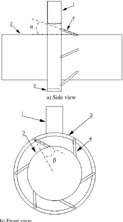
Fig. 1. The pump is configured to use compressed air as the primary fluid. The primary inlet pipe (1) which is connected to an air-line. The annulus (3) of the pump is filled to the desired air pressure. This stored energy is then transferred via the nozzles (4) to the pipe bore (2).

a) Side view

b) Front view

Figure 1. Multi-nozzle annular jet pump

1. Primary Inlet Pipe 2. Pipe Bore

3. Annulus 4. Nozzles

α: Axial angle β: Radial angle

The efficiency of a jet pump is described as the ratio of energy transferred to the secondary fluid over the energy lost by the primary fluid. One-dimensional models, defined by Eqs. (1) to (3), characterise the jet pumps performance [2]. Flow variables are given in the nomenclature and location within the flow detailed in Figure 2.

𝑀 = 𝑄𝑠

𝑄𝑝 (1)

𝑁 =(𝑃𝑑− 𝑃𝑠) (𝑃𝑝− 𝑃𝑑)

(2)

𝜂 = 𝑀 × 𝑁 = 𝑄𝑠(𝑃𝑑− 𝑃𝑠) 𝑄𝑝(𝑃𝑝− 𝑃𝑑)

(3)

The effect of swirl, or vortical flow, for a traditional AJP design was experimentally tested by Shimizu [3]. The study concluded that an intensive swirl was detrimental to the pumps efficiency, whereas a moderate swirl resulted in greater efficiency caused by increased entrainment between primary and secondary fluids. Notably, a weak swirl resulted in no effect on the efficiency. Further studies on the effect of a swirling primary fluid in jet support these results [4]. Conversely, Zhou [5] showed numerically that swirl was detrimental to pump performance. Moreover, studies support that a moderate swirling flow increases fluid entrainment and hence can be used to increase a jet pumps efficiency.

Such, the design of the multi-nozzle AJP can be improved by finding the optimal level of swirl. This study, based on experimental analysis and numerical simulations forms a baseline of method and analysis, from which design development can be undertaken to find the optimal orientation of nozzles for maximum entrainment. Two initial designs, called Prototypes 1 and 2, corresponding to Fig. 1, are tested. The prototype multi-nozzle AJPs are compared and validated through CFD and experimental analysis. The performance and efficiency of the pumps and the flow characteristics are analysed by comparing the effects of single-phase air-air flow. Pressurised air is considered as the primary fluid which, when injected into the pump draws and entrains the secondary fluid, atmospheric air. The pressure of the primary fluid is adjusted and the subsequent effects observed, notably the change in pump suction and output pressure. CFD analysis is used to complete equations 1-3 by determining the volume flow rate in addition to other flow variables. CFD simulations consider the sensitivity of grid-independent solutions to selected turbulence models to validate the numerical method against experimental analyses. Unsteady hybrid turbulence models are compared against steady and unsteady RANS based turbulence models.

This paper starts by detailing the apparatus used for the analyses, including the pump design, the test rig for experiments, and the software and methods for numerical simulations. In sections 5 and 6 the results from the experiments and simulations are presented with results compared for the validation of numerical methods. A summary of the work is detailed in the final section with remarks regarding future work.

α

2. TEST RIG

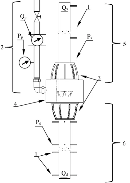
Figure 2 illustrates the test rig setup; consisting of the multi-nozzle AJP, two unequal length pipes connect either side of the pump by means of sealed pipefittings. 27 pressure taps connected to a fluid column manometer measure the static wall pressure at various intervals. 11 pressure taps are linearly distributed on the inlet pipe with 16 circumferentially placed on the output pipe. Pressure taps are flush mounted against the pipe wall such that they are non-intrusive, ensuring no disruption to the flow through the pipe bore. The manometer reading error is taken as ± the minor scale graduation of the manometer scale, ±30Pa. The pressure taps are 25 mm from the inlet/outlet, spaced 100 mm apart along the pressure pipe and 50 mm apart along the suction pipe. To measure the primary flow into the pump a pressure gauge and volume flow meter are connected upstream on the compressed air line. The pressure of the primary fluid entering the pump is increased by 0.5 bar up to 4 bar by adjusted a pressure valve.

Figure 2. Experimental Rig

1. Pressure Taps

2. Compressed air line (Primary Fluid Inlet) 3. Air-tight connection fittings

4. Multi-nozzle Annular Jet Pump 5. Suction pipe (Inlet Pipe) 6. Pressure pipe (Outlet Pipe)

2.1 Multi-nozzle Annular Jet Pump

Referring to Fig. 1, the annular chamber of the pumps forms a plenum, storing the primary fluid at the desired upstream pressure. The nozzles convert this pressure into kinetic energy, which is subsequently imparted to the secondary fluid in the pipe bore. The two fluid streams mix and exchange energy resulting a combined output flow.

The configuration and dimensions of the pumps are given in Fig. 1, and Table 1. Using the axial angle α and the radial angle β indicated in Fig. 1, the Nozzle angle ratio δ is defined as:

𝛿 =𝛼

𝛽 (4)

Table 1. Experimental Rig & Pump Dimensions

Pump Geometry Dimension

Pipe Bore Diameter 50 mm

Primary Inlet Pipe Diameter

1/2 Inch BSP

(12.7 mm)

Number of Nozzles 6

Nozzle Diameter 2 mm

δ Prototype 1: 1.75

Prototype 2: 3.00

Inlet Pipe Length 600 mm

Inlet Pipe Diameter 50 mm

Outlet Pipe Length 700 mm

Outlet Pipe Diameter 50 mm

Total Domain Length 1.43 m

The two prototypes use a different nozzle orientation to determine the influence on the AJP performance. Prototype 1 has a smaller axial angle than Prototype 2, giving the jet velocity a larger axial component. The radial angle is the same for the two devices.

3. CFD CODE

The CFD simulations herein use the commercial finite volume code ANSYS® _{FLUENT, Release} 17.2, and consider a single-phase analysis representative of the conditions in the experiments. All analyses use a compressible flow model. The space-discretisation of the governing equations is second order accurate, and, in the case of unsteady flow simulations, the time-resolution is second order accurate. The pressure based, COUPLED solver is Ps

Pp

Pd Qp

Qs

Qd

1

1 2

3

4

5

used for the numerical integration, Chapter 20, page 685 [6].

3.1. Turbulence Modelling

Steady mode analyses

For the steady state analyses, two Reynolds-averaged Navier-Stokes (RANS) models are used, the k-ω Shear Stress Transport (SST) model and the Reynolds Stress Model (RSM). The k-ω SST model combines the benefits of both k-ε and k-ω models, enabling integration of the turbulence model all the way down to solid wall boundaries without wall functions, ensuring a good level of solution insensitivity to the value of the specific dissipation rate ω enforced on far field boundaries. The RSM model is used because, although computationally more demanding than linear eddy viscosity models, has been reported as a promising model in the prediction of swirling flows [7], and is also recommended for this type of flow in the ANSYS® Fluent theory guide; Chapter 4, Page 83 [6].

Unsteady mode analyses

Transient simulations are carried out with the aforementioned RANS models used in steady mode. Additionally, the Scale-Adaptive Simulation (SAS) method [8] and the Delayed Detached Eddy Simulation (DDES) [9] are used. Both models are hybrid methods achieving a trade-off between the higher resolution of Large Eddy Simulations and the high computational performance of RANS simulations, using the k-ω SST as the sub-grid scale model [10]. A time step size of 1-5 _{seconds is used} for all transient simulations [11]. The number of iterations per time step is set at 100, which was found to produce sufficient convergence to the residual level. The temporal discretisation method for the RANs based models is second order implicit, with the bounded second order implicit method required for SAS and DDES simulations, Chapter 4, Page 92-98 [6].

4. NUMERICAL SETUP

4.1. Computational Domain & CFD Grid

The fluid domain replicates the experimental set-up and is illustrated in Figure 3. The length of the compressed air line is 2.5 m from the pump to the pressure gauge and flow meter. To reduce computational costs, the length of the primary inlet pipe is decreased, assuming pressure indicated upstream of the pump is the same as that entering the pump. The cyclic symmetry assumption of the flow is not used, despite the fact that this would enable a reduction of the computational domain by a factor equal to the number of jets. Assessing the viability of

this modelling option for this problem is part of ongoing work.

Figure 3. Computational Domain.

1. Primary inlet 2. Secondary inlet 3. Outlet

4. Nozzles

5. Annulus 6. Pressure pipe 7. Suction pipe 8. Pump Bore

4.2. Boundary Conditions

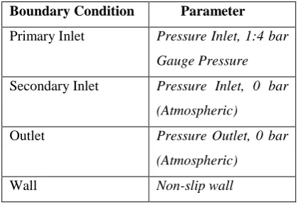
The boundary conditions are shown in Table 2 and refer to Fig. 3.

Table 2. Boundary Conditions.

Boundary Condition Parameter

Primary Inlet Pressure Inlet, 1:4 bar Gauge Pressure

Secondary Inlet Pressure Inlet, 0 bar (Atmospheric)

Outlet Pressure Outlet, 0 bar (Atmospheric)

Wall Non-slip wall

5. EXPERIMENTAL RESULTS

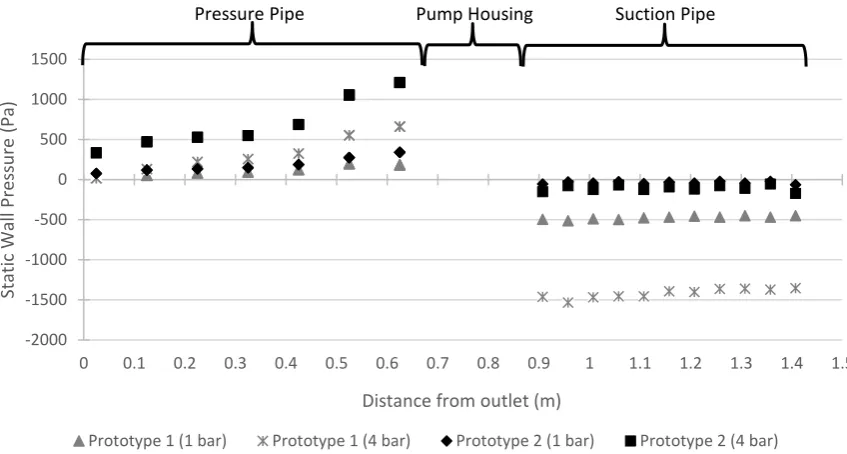
The two designs (Prototypes’ 1 and 2) are compared in Fig. 4, reporting the wall static pressure at intervals along the suction and pressure pipes for the two devices operating at different total pressure. Prototype 1 produces a significantly larger suction pressure, signifying the importance of using a lower axial angle in producing a high vacuum pressure. In the pressure side of the pump, Prototype 2 produces a higher value. For both devices, the pressure in the pressure pipe increases as the pressure of the compressed air increases; increasing this variable, however, results in lower pressure (and thus higher velocity and secondary fluid volume flow) only for Prototype 1, pointing to a better performance of this device.

1

2

3 5

4

Suction pipe

Pressure pipe

6

7

Figure 4. Experimental static wall pressure, suction and pressure pipes.

6. CFD ANALYSES

6.1. Mesh refinement and mesh

sensitivity analyses

The grid independence of the CFD solutions is assessed using a grid refinement and topology study. Three levels of refinement are considered for two different meshing methods. These methods are considered to investigate the possibility of improving further the agreement between simulations and measurements. For both cases, the boundary layer is simulated by ensuring adequate cell count through inflation layering along all walls, so that the non-dimensionalised wall distance y+ of the first nodes off all solid walls be of order 1 in all cases.

The first mesh type, named the hybrid mesh in this study, constitutes of several domains built using structured and unstructured grids. The hybrid coarse, medium and fine grids have, respectively 5.0, 10.0, and 20.0 million cells. The benefit of this meshing method is higher flexibility in controlling the element density, concentrating more cells in the areas of complex fluid flow, such as in the annulus, nozzles and pipe bore where the total cell count is 3.8, 7.6 and 16.3 million for the coarse, medium and fine grids respectfully. For the hybrid mesh, the nozzles, primary inlet pipe, the pressure pipe and suction pipes use a structured hexahedral grid. The annulus and pump bore is generated using an unstructured tetrahedral grid.

The second mesh is a single domain tetrahedral

unstructured grid. The advantage of this grid type is that it enables greater boundary layer refinement,

incorporating more and higher quality inflation layers past sharp geometric corners. Whereas the

hybrid mesh is created from individual domains, requiring interfaces between parts so that a sharp geometric change between the interface and domains constrains the level of boundary layer refinement by limiting the number of cells in the boundary layer between adjacent regions. Conversely, the

unstructured grid meshes the entire domain collectively, producing a higher mesh quality, although this is at considerably greater computational cost, with 11.4, 20.4, 29.5 million cells for the coarse, medium and fine grids respectfully.

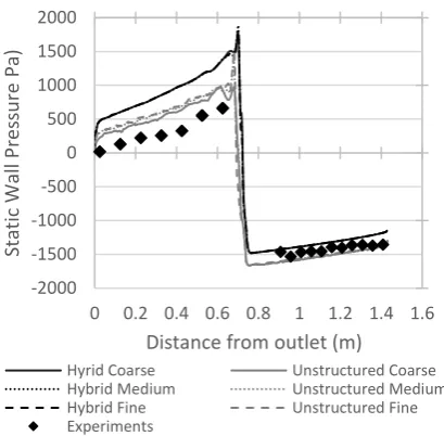
In Figures 5 and 6, the wall static pressure distributions computed with the hybrid and

unstructured meshes are plotted against the experimental data for Prototype 1 and 2 respectfully. These numerical results refer to the steady state k-ω

SST simulations with the gauge pressure of the primary inlet boundary condition set at 4 bar. The results of Figs. 5 and 6 show that for both grid topologies, the coarse grid refinement is adequate for obtaining grid-independent results. The results of these figures also highlight a very good prediction of the general experimental trends, and a good quantitative agreement between measurements and simulations. It is noted, however, that the quantitative agreement between CFD and measured data varies with the considered operating conditions, as highlighted in section 6.2. The unstructuredmesh

topology shows slightly better agreement with experiments, however due to time constraints the

hybridmesh is used for most of the analyses reported below.

-2000 -1500 -1000 -500 0 500 1000 1500

0 0.1 0.2 0.3 0.4 0.5 0.6 0.7 0.8 0.9 1 1.1 1.2 1.3 1.4 1.5

Sta

tic W

all

Pres

su

re

(Pa)

Distance from outlet (m)

Prototype 1 (1 bar) Prototype 1 (4 bar) Prototype 2 (1 bar) Prototype 2 (4 bar)

Figure 5. k-ω SST Grid refinement and sensitivity analyses, Static wall pressure, Prototype 1. 4 bar

primary pressure.

Figure 6. k-ω SST Grid refinement and sensitivity analyses, Static wall pressure, Prototype 2. 4 bar

primary pressure.

6.2. Turbulent model sensitivity

analyses

To cross-validate computed results and measured data, the CFD wall static pressure distributions for various turbulence models is compared using the hybrid mesh.

The static wall pressure is compared using the steady and unsteady RANS turbulence models in Figures 7-8 for Prototypes 1 and 2 respectfully. Results indicate that there is little difference between the unsteady/steady methods for the respective turbulence models. Although, the pump is shown to

be sensitive to turbulence modelling. In Fig. 7, Prototype 1, the RSM model predicts a smaller suction pressure and a higher output pressure compared to the k-ω SST model. In Fig. 8, Prototype 2, also shows a sensitivity to the selected turbulence model, though contrary to Fig. 8, the RSM model calculates a lower output pressure than that of k-ω SST model. In both cases, the RSM model predicts a fluctuating pressure downstream of the primary fluid injection.

Figure 7. Prototype 1, Steady vs. Unsteady, Static wall pressure; 2 bar gauge primary fluid

pressure.

Figure 8. Prototype 2, Steady vs. Unsteady RANS, Static wall pressure; 2 bar gauge primary

fluid pressure.

For the unsteady analysis, simulations are run for a number of time steps until monitor points within the flow have reached a steady solution. Monitor points are located at points of interest in the flow field to detect changes in pressure and velocity with each time step.

-2000 -1500 -1000 -500 0 500 1000 1500 2000

0 0.2 0.4 0.6 0.8 1 1.2 1.4 1.6

Sta

tic W

all

Pres

su

re

Pa

)

Distance from outlet (m)

Hyrid Coarse Unstructured Coarse

Hybrid Medium Unstructured Medium

Hybrid Fine Unstructured Fine

Experiments

-1000 0 1000 2000 3000 4000 5000 6000 7000

0 0.2 0.4 0.6 0.8 1 1.2 1.4 1.6

Sta

tic W

all

Pres

su

re

(Pa)

Distance from outlet (m)

Hyrid Coarse Unstructured Coarse

Hybrid Medium Unstructured Medium

Hybrid Fine Unstructured Fine

Experiments

-1000 -800 -600 -400 -200 0 200 400 600 800 1000

0 0.2 0.4 0.6 0.8 1 1.2 1.4 1.6

Sta

tic W

all

Pres

su

re

(Pa)

Distance from outlet (m)

Steady RSM Unsteady RSM

Steady K Omega SST Unsteady K Omega SST

Experiments

-500 0 500 1000 1500 2000 2500 3000 3500

0 0.2 0.4 0.6 0.8 1 1.2 1.4 1.6

Sta

tic W

all

Pres

su

re

(Pa)

Distance from outlet (m)

Steady RSM Unsteady RSM

Steady K Omega Unsteady K Omega SST

SAS and DDES results for Prototype 1 obtained using the unstructuredgrid are shown in Figure 9, cross-comparing the unsteady RANS pressure profiles of Fig. 7 highlights that a notable improvement of the wall static pressure profiles is achieved by using these hybrid models.

Figure 9. Prototype 1, Transient, Static wall pressure; 2 bar gauge primary fluid pressure.

Simulations show that the static wall pressure in the pressure pipe fluctuates downstream, both spatially and temporally. Fluctuations are observed for both prototypes and indicate that the output from the pump is swirling and unsteady. The fluctuations vary and range up to ± 50 Pa. The pressure in suction pipe does not fluctuate, implying that the flow into the pump is constant.

6.3. Pump Efficiency Curve

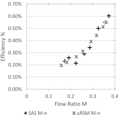
The efficiency of the pump is represented through characteristic curves based on equations (1) to (3). The efficiency (η) vs. flow ratio (M) curve, shown in Figure 10, compares the results of the SAS and unsteady RSM turbulence models obtained for the more efficient Prototype 1. The relative low jet pump efficiency of the multi nozzle AJP is attributed to the size of the ratios M and N defined by Eqs. (1) to (2) respectfully.

The pressure ratio is predominately affected by the primary pressure, Pp, in the denominator of Eq. (2). Pp takes a gauge value between 50 and 400 kPa, significantly larger than the values Ps and Pd in the numerator for which values range between 0.02 to 4 kPa. The magnitude of Ps and Pd increase by a moderate amount with respect to each other, which can be seen in the static pressure distribution curves in Figs. (4-10). Thus, it is found that N is in the order of 10-2_.

The flow ratio M was also found to be small with Qp significantly larger than the Qs giving a ratio in the order of magnitude of 10-1_{, impacting the} calculated jet pump efficiency. It was found that increasing the primary fluid pressure resulted in a linear increase of M. This suggests that the entrainment between secondary and primary fluids improved with higher pressures.

Figure 10. Prototype 1, M-η curve.

6.4. Detailed Flow Analysis

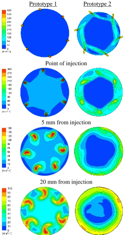
The first row of subplots of Figure 11 shows contour plots of velocity magnitude in the transverse section at the injection point of Prototypes 1 and 2, whereas the subsequent four rows of subplots compare the contours of the same variable at 5, 20, 35 and 100 mm downstream of the injection point for the two prototypes. The gauge pressure of the compressed air is 2 bar in both cases. The plots are used to analyse the effects of the nozzle orientation on the AJP flow patterns, emphasising the primary and secondary flow interaction and showing how the structure of the developing flow differs between prototypes.

For both prototypes, the nozzle jets expand exchanging momentum with the secondary stream. The high-pressure fluid, ejected from the nozzles as a discrete jet gradually develops into an annulus on the periphery of the pipe, though this occurs at different rates for the two prototypes.

Due to the higher axial angle of the nozzles in Prototype 2, a significant radial velocity is imparted to the flow. This is evident already at the injection point (first row of subplots), showing that the jets of Prototype 1 have a very coherent pattern, whereas those of Prototype 2 have already merged significantly in the circumferential direction. At 5 mm downstream of the injection point, the velocity in the central part is already significant (indicating

-1000 -800 -600 -400 -200 0 200 400 600 800 1000

0 0.2 0.4 0.6 0.8 1 1.2 1.4 1.6

Sta

tic W

all

Pres

su

re

(Pa)

Distance from outlet (m)

DDES SAS Experiments

0.00% 0.10% 0.20% 0.30% 0.40% 0.50% 0.60% 0.70%

0 0.1 0.2 0.3 0.4

Ef

fici

en

cy

%

Flow Ratio M

greater suction), whereas the fluid in the same region is motionless in the case of Prototype 2, a feature highlighting the higher effectiveness of Prototype 1. At 20 mm from the injection point, the higher momentum exchange between jets and secondary flow results in the area of non-zero flow velocity growing further, for Prototype 1, with respect to the previous axial position, whereas the growth of the secondary fluid velocity is substantially lower in the case of Prototype 2. Moreover, for Prototype 1, the jets are still coherent and little circumferential uniformity exists. The most striking flow feature at 35 mm downstream of the injection point, is that the footprints of the jets of Prototype 1 start deforming circumferentially, a result of the swirling flow component imparted to the mixed stream. At the position 100 mm downstream of the injection point, the circumferential mixing of the jets of Prototype 1 is advanced but not complete, as the jet footprints are still distinguishable, whereas the circumferential mixing of the jets of Prototype 2 is complete and the velocity in the central part of the duct is still zero, indicating extremely poor suction.

Prototype 1 Prototype 2

Point of injection

5 mm from injection

20 mm from injection

35 mm from injection

100 mm from injection

Figure 11.Comparison of prototypes, Velocity contours, 2 bar primary fluid pressure.

7. CONCLUSIONS

Two multi-nozzle AJPs are tested experimentally and numerically. Experimental and numerical results showed a similar trend: increasing the pressure of the primary fluid resulted in higher suction pressure and output pump pressure. This pattern is common to both considered prototypes, but the extent of this effect was found to vary significantly with the AJP design. Efficiency of the pump is low due to the low levels of both the pressure and the flow ratios. However, experimentally validated CFD can drive AJP design aiming at maximising its performance.

The turbulence model analysis has shown that there is little difference between the steady state and transient RAN’s models tested. The hybrid SAS and DDES models, though, show significant improvement compared against experiments, but at a greater computational cost. Computation time may be offset in future analysis, as the pump is shown to be cyclically symmetrical allowing the domain to divided into sectors. Further analysis on the

unstructured based meshing method is required to match experimental data more closely. Additionally, uncertainty analysis looking into manufacturing tolerances will be looked into to reduce the offset between results.

ACKNOWLEDGEMENTS

This work is supported by the Centre for Global Eco Innovation and the ERDF. Design of the multi-nozzle AJP is credited to TCL Cumbria with which this work is presented in partnership. Special thanks to industry advisor, Ian Stephenson.

REFERENCES

[1] Cunningham, R. G. (2000). Jet Pump Applications. In I. J. Karassik, J. P. Messina, P. Cooper, & C. C. Heald, Pump Handbook. New York: McGraw-Hill.

[3] Shimizu, Y., Nakamura, S., Kuzuhara, S., & Kurata, S. (1987). Studies of the Configuration and Performance of Annular Type Jet Pumps. 109(3).

[4] Guillaume, D, and Judge. “Improving the Efficiency of a Jet Pump Using a Swirling Primary Jet.” Review of Scientific Instruments, vol. 75, no. 2, 2004, pp. 553–555.

[5] Zhou, B., Fleck, B., Bouak, F., & Gauthier, J. (2000). Comparison of swirling effects on ejector performance using four turbulence models.

Canadian Aeronautics and Space Journal, 46(4), 178-182.

[6] ANSYS® Academic Research Fluent, 17.2, Theory Guide.

[7] Hirai, S., Takagi, T., & Matsumoto, M. (1988). Predictions of the Laminariazation Phenomena in an Axially Rotating Pipe Flow.

110(4).

[8] Menter, F, and Y Egorov. “Revisiting the Turbulent Scale Equation.” Solid Mechanics and Its Applications, vol. 129, 2006, pp. 279–290

[9] Spalart, P., et al. “A New Version of Detached-Eddy Simulation, Resistant to Ambiguous Grid Densities.” Theoretical and Computational Fluid Dynamics, vol. 20, no. 3, 2006, pp. 181–195.

[10] Strelets, M. “Detached Eddy Simulation of Massively Separated Flows.” 39th Aerospace Sciences Meeting and Exhibit, 2001.