Spatio temporal Bayesian on line changepoint detection with model selection

warwick.ac.uk/lib-publications

Original citation:

Knoblauch, Jeremias and Damoulas, Theodoros (2018) Spatio-temporal Bayesian on-line

changepoint detection with model selection. In: 35th International Conference on Machine

Learning 2018, Stockholm, Sweden, 10-15 Jul 2018. Published in: Proceedings of the 35th

International Conference on Machine Learning 2018 (In Press)

Permanent WRAP URL:

http://wrap.warwick.ac.uk/102761

Copyright and reuse:

The Warwick Research Archive Portal (WRAP) makes this work of researchers of the

University of Warwick available open access under the following conditions.

This article is made available under the Creative Commons Attribution 4.0 International

license (CC BY 4.0) and may be reused according to the conditions of the license. For more

details see:

http://creativecommons.org/licenses/by/4.0/

A note on versions:

The version presented in WRAP is the published version, or, version of record, and may be

cited as it appears here.

Jeremias Knoblauch1 Theodoros Damoulas1 2 3

Abstract

Bayesian On-line Changepoint Detection is ex-tended to on-line model selection and non-stationary spatio-temporal processes. We pro-pose spatially structured Vector Autoregressions (VARs) for modelling the process between changepoints (CPs) and give an upper bound on the approximation error of such models. The resulting algorithm performs prediction, model selection and CP detection on-line. Its time com-plexity is linear and its space comcom-plexity constant, and thus it is two orders of magnitudes faster than its closest competitor. In addition, it outperforms the state of the art for multivariate data.

1. Introduction

Real-world spatio-temporal processes are often poorly mod-elled by standard inference methods that assume stationarity in time and space. A variety of techniques have been devel-oped for modelling non-stationarity in time via changepoints (CPs), ranging from methods for Gaussian Processes (GPs) (Garnett et al., 2009), the Lasso (Lin et al., 2017) or the Ising model (Fazayeli & Banerjee, 2016) over approaches using density ratio estimation (Liu et al., 2013) and kernel-based methods exploiting M-statistics (Li et al., 2015) to framing CP detection as time series clustering (Khaleghi & Ryabko, 2014). In contrast, CP inference allowing for non-stationarity in space (Herlands et al., 2016) has received comparatively little attention.

We offer the first on-line solution to this problem by model-ing non-stationarity in both space and time. CPs are used to model non-stationarity in time, and the use of spatially structured Bayesian Vector Autoregressions (SSBVAR) cir-cumvents the assumption of stationarity in space. We unify the approaches in Adams & MacKay (2007) and Fearnhead

1

Department of Statistics, University of Warwick, UK

2

Department of Computer Science, University of Warwick, UK

3

The Alan Turing Institute for Data Science, UK. Correspondence to: Jeremias Knoblauch<[email protected]>. To appear in Proceedings of the35th

International Conference on Machine Learning, Stockholm, Sweden, PMLR 80, 2018. Copy-right 2018 by the author(s).

0 10

Value

0 2

PE

0

1

P(m|y)

0 100 200 300 400 500

0

100

200

run length

AR(2) AR(3) VAR4(2) VAR8(1)

-1000 -99 -89 0

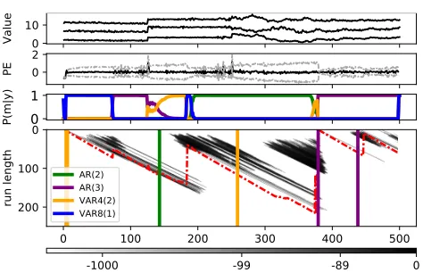
Figure 1.Bayesian On-line Changepoint Detection with Model Se-lection (BOCPDMS):Panel 1:Artificial data across times1−500 for a regular spatial grid with4- and8-neighbourhood dependency structure as in Fig. 2,Panel 2:prediction error (black) and vari-ance (gray).Panel 3:Model posteriorsP(mt|y1:t).Panel 4:log

run-length distribution (grayscale), its maximum (red) and MAP segmentation of CPs and models in corresponding colors.

& Liu (2007) by building a flexible algorithm with three on-line outputs: prediction,model posteriorsand aMAP segmentationfor CPs and models. This conjunction is pos-sible as both methods build on the Product Partition Model (Barry & Hartigan, 1993). The inputs for the algorithm are a multivariate data stream{Yt}and a set of Bayesian

models Mthat describe the data between CPs. The al-gorithm’s advantages over other procedures are threefold: Firstly, it performs better than competing algorithms at a fraction of the computational cost. Secondly, we distinguish between data generating mechanisms with different and interpretable parameterizations via Bayesian model selec-tion. Thirdly, the algorithm lends itself naturally to efficient high-dimensional spatio-temporal inference using spatial neighbourhoods.

In spirit, our work is similar to Xuan & Murphy (2007), which performs automaticoff-linemodel selection and in-ference on dependent multivariate time series. In particular, their dependence is modelled using correlated errors in au-toregressions. The approach requires conjugate priors to scale, restricting the dependency patterns to decomposable graphs. In contrast, our inference procedure requires specifi-cation of a model universeMbefore running the algorithm,

but inference ison-line. Crucially, no restrictions are im-posed on dependencies inM. This is achieved by modelling dependencyconditionallyrather thancontemporaneously.

The second line of related research is developed in Saatc¸i et al. (2010), which extends the Bayesian On-line Change-point Detection (BOCPD) algorithm of Adams & MacKay (2007) to Gaussian Process (GP) CP models. These are compatible with our framework as elements of the model universeM. However, GPs incur additional computational cost, increasing the overall complexity by two orders of magnitude. The proposed approach avoids this and outper-forms the state of the art in the multivariate setting, while offering comparable performance in the univariate one.

The structure of this paper is as follows: Section 2 gener-alizes the BOCPD algorithm of Adams & MacKay (2007), henceforth AM, by integrating it with the approach of Fearn-head & Liu (2007), henceforth FL. In so doing, we arrive at BOCPD with Model Selection, henceforth BOCPDMS. Sec-tion 3 proposes VAR models for non-staSec-tionary processes within the BOCPD framework. This motivates populat-ing the model universeMwith spatially structured BVAR (SSBVAR) models. Sections 4–5 address computational aspects. Section 6 demonstrates the algorithm’s advantages on real world data.

2. BOCPDMS

Let{Yt}be a data stream with an unknown number of CPs.

Focusing on univariate data, FL and AM tackled inference by tracking the posterior distribution for the most recent CP. While FL allow the data to be described by different models between CPs, AM only allow for a single model. However, AM perform1-step-ahead predictions, whereas FL do not. Instead, they propose a Maximum A Posteriori (MAP) segmentation for CPs and models. In the remainder of this section, we unify both inference approaches. We call the resulting algorithm BOCPD with model selection (BOCPDMS), as it performs prediction, MAP segmentation and model selection on-line.

2.1. Run-length & model universe

Therun-lengthrtat timetis defined as the time since the

most recent CP at timet, sort = 0corresponds to a CP

at timet. Suppose that data between successive CPs can be described by Bayesian models collected in themodel universeM. For the process{Yt}onRS, a modelm∈ M consist of a conditional probability densitydP(Yt|θm)on

RSand a parameter prior densitydP(θm)onΘmdepending

on hyper-parametersθ0

m. The notion ofMis due to FL and

allows for model uncertainty amongst models developed for BOCPD. For instance,m∈ Mcould be a GP (Saatc¸i et al., 2010), a time-deterministic regression (Fearnhead, 2005) or

a mixture distribution (Caron et al., 2012).

BOCPD with Model Selection (BOCPDMS)

Input at time0:model universeM; hazardH; priorq Input at timet:next observationyt

Output at timet:y_b(t+1):(t+hmax),St,P(mt|y1:t)

for next observationytat timetdo

//STEP I: Compute model-specific quantities for m∈ M do

if t−1 =lag length(m) then

I.A Initialized_P(y1:t, rt= 0, mt=m)with prior

else if t−1>lag length(m) then

I.B.1 Updated_P(y1:t, rt, mt=m)via (5a), (5b)

I.B.2 Prune model-specific run-length distribution I.B.3 Perform hyperparameter inference via (12)

end if end for

//STEP II: Aggregate over models if t >= min(lag length(m)) then

II.1 Obtain joint distribution overMvia (6a)–(6f) II.2 Compute (7)–(9)

II.3 Output:y_b(t+1):(t+hmax), St,P(mt|y1:t)

end if end for

2.2. Probabilistic formulation & recursions

Denote bymtthe model describingy(t−rt):t, i.e. the data

since the last CP. Given hazard functionH : N →[0,1], and model priorq:M →[0,1], the prior belief is

P(rt|rt−1) =



 

 

1−H(rt−1+ 1) ifrt>0

H(rt−1+ 1) ifrt= 0

0 otherwise. (1a)

P(mt|mt−1, rt) =

(

1mt−1(mt) ifrt>0 q(mt) ifrt= 0.

(1b)

Eq. (1b) implies that the model at timetwill be equal to the model at timet−1unless a CP occured att, in which case the next modelmtwill be a random draw fromq. At

timet, the algorithm requires for all possible modelsmt

and run-lengthsrtthe computation of the densities

dP(yt|y1:(t−1), mt, rt) =

Z

Θ_mt

dP(yt|θmt)dP(θmt|y(t−rt):(t−1))dθmt. (2)

which make the following recursion efficient, too:

dP(y1:t, rt, mt) =

X

mt−1

X

rt−1

n

dP(yt|y1:(t−1), rt, mt)P(mt|y1:(t−1), rt, mt−1)

P(rt|rt−1)dP(y1:(t−1), rt−1, mt−1)

o

. (3)

The recursion in AM is the special case for|M|= 1. For |M| > 1,P(mt|mt−1, rt,y1:(t−1))arises as a new term, which for1aas the indicator function ofais given by

(

1mt−1(mt)P(mt−1|y1:(t−1), rt) ifrt>0

q(mt) ifrt= 0.

(4)

Next, define thegrowth-andchangepoint probabilitiesas

d_P(y1:t, rt=rt−1+ 1, mt) =

dP(yt|y1:(t−1), rt, mt)dP(y1:(t−1), rt−1, mt−1)×(5a)

(1−H(rt))P(mt−1|y1:(t−1), rt),

dP(y1:t, rt= 0, mt) =

dP(yt|y1:(t−1), rt, mt)q(mt)× (5b)

X

mt−1

X

rt−1

n

H(rt−1+ 1)dP(y1:(t−1), rt−1, mt−1)

o

.

The evidence can then be calculated via Eq. (6a), which in turn allows calculating the joint model-and-run-length distribution (6b), the model posterior (6c), as well as the model-specific (6d) and global (6e) run-length distributions:

d_P(y1:t) =Pmt P

rtdP(y1:t, mt, rt) (6a)

P(rt, mt|y1:t) =dP(y1:t, rt, mt)/dP(y1:t) (6b)

P(mt|y1:t) =PrtP(rt, mt|y1:t) (6c)

P(rt|mt,y1:t) =dP(rt, mt|y1:t)/dP(mt|y1:t)(6d)

P(rt|y1:t) =P_mtP(rt, mt|y1:t) (6e)

P(mt−1|y1:(t−1), rt) =

P(mt−1, rt−1|y1:(t−1))

P(rt−1|y1:(t−1))

. (6f)

Eq. (6f) is the conditional model posterior from Eq. (4). Eq. (6e) is arrived at directly in FL and used for on-line MAP segmentation. By framing our derivations in the run-length framework of AM, we additionally obtain (4)–(6d), thus enabling on-line prediction and model selection at the same computational cost.

2.3. On-line algorithm outputs

Prediction:Recursiveh-step-ahead forecasting uses (6b):

d_P(Yt+h|y1:t) =

X

rt X

mt n

dP(Yt+h|y1:t,yb

h

t, rt, mt)P(rt, mt|y1:t)

o

, (7)

wherey_bh_t =∅ifh= 1andy_bth=y_b(t+1):(t+h−1)otherwise, withy_bt+h=E(Yt+h|y1:t,yb

h

t)the recursive forecast.

Tracking the model posterior/Bayes Factors:One of the novel capabilites of the algorithm is on-line monitoring of the model posterior via Eq. (6c). This is attractive when structural changes in the data happen slowly and are not captured well by CPs. In this case,P(mt|y1:t)can be used

to identify periods of change, see Fig. 6. For pairwise comparisons, Bayes Factors can be monitored, too:

BF(m1,m2)t=

P(mt=m1|y1:t)·q(m2)

P(mt=m2|y1:t)·q(m1) . (8)

Maximum A Posteriori (MAP) segmentation:For MAPt

the density of the MAP-estimate attand MAP0= 1, FL’s recursive MAP estimator is given by

MAPt= max r,m

n

dP(y1:t, rt=r, mt=m)MAPt−r−1

o

. (9)

Forr∗

t, m∗tmaximizers for timet, the MAP segmentation is

St=St−r∗

t−1∪ {(t−r

∗

t, m∗t)},S0=∅, where(t0, mt0)∈

Stmeans a CP att0≤t, withmt0 ∈ Mthe model fory_t0_:t.

3. Building a spatio-temporal model universe

The last section derived BOCPDMS for arbitrary data streams{Yt}. Next, we propose models forMif {Yt}

can be mapped into a space _S. LetS with |S| = S be a set of spatial locations in S with measurements Yt =

(Yt,1, Yt,2, . . . , Yt,S)T recorded at timest= 1,2, . . .

3.1. Bayesian VAR (BVAR)

Inference on{Yt}can be drawn using conjugate Bayesian

Vector Autoregressions (BVAR) with lag lengthLandE additional variablesZtas elements of model universeM:

σ2∼InverseGamma(a, b) (10a)

εt|σ2∼ N(0, σ2·Ω) (10b)

c|σ2∼ N(0, σ2·Vc) (10c)

Yt=α+BZt+P L

l=1AlYt−l+εt. (10d)

Here, Al,B are S × S, S × E matrices, c =

(α,vec(B),vec(A1),vec(A2), . . .vec(AL))T is a vector

ofS·(LS+ 1 +E)model parameters. Scalarsa, b >0, matrixVc, and diagonal matrixΩare hyperparameters.

3.2. Approximating processes using VAR

Modelling{Yt} as VAR is attractive, as many complex

Theorem 1. Let {Yt} be a time-stationary spatio-temporal process with spectral density satisfying regularity condition (A) of Meyer & Kreiss (2015),

|| · || a matrix norm, E(Yt) = 0, E(YtYtT) < ∞,

P∞

h=−∞(1 +|h|)3||E[YtYt0+h]||<∞. Then (1)–(3) hold.

(1) Yt = P∞i=1AiYt−i+εtfor matrices{Al}l∈Nand E(εt) = 0,E(εtε0t) =D,Ddiagonal.

(2) For Yt = P L l=1A

L

lYt−l + et with {ALl} L l=1 the

best linear projection coefficients,∃L0 : ∀L > L0,

PL

l=1(1 + |l|)

3_||AL

l −Al|| ≤ C · P

∞

l=L+1(1 +

|l|)3_||A

l||withCconstant.

(3) Using T observations with L = O([T /ln(T)]1/6)

to estimateAL

l as the MAP AbL_l of (10a)–(10d), it

holds thatL(T)2PL(T)

l=1 ||Ab

L(T)

l −A

L(T)

l ||

P

→ 0as

T → ∞.

Proof. Part (1) is shown in Inoue et al. (2018), part (2) in Lemma 3.1 of Meyer & Kreiss (2015). Part (3) fol-lows by their Remark 3.3 if we can prove that the MAP estimatorc(L(Tˆ ))ofcequals its Yule-Walker estimator (YWE) as T → ∞. Let B = 0, α = 0 and note that YWE equals OLS as T → ∞. With X1:T the

re-gressor matrix of Yt−L(T):t, c(L(Tˆ )) = (X1:0TX1:T +

Vc−1)−1(X1:0TY1:T). Then, part (3) holds as OLS P

→ E(X1:0TX1:T)−1E(X1:0TY1:T)and

ˆ

c(L(T)) = (X_1:0_TX1:T +Vc−1)−

1_(X0

1:TY1:T)

= (1 TX

0

1:TX1:T+

1 TV

−1

c )−

11

T(X 0

1:TY1:T)

P

→E(X1:0TX1:T)−1E(X1:0TY1:T).

In Thm. 1, assuming_E(Yt) =0is without loss of

general-ity: If_E(Yt) =α+BZt, defineYt∗=Yt−(α+BZt)and

apply the theorem to{Y_t∗}. Moreover, the results donot

require stationarity in space. Lastly, part (3) suggests a prin-cipled way of picking lag lengthsLfor BVAR models: If betweenT1andT2observations are expected between CPs, L={L∈N:L(T1)≤L≤L(T2)}. In the experiments of section 6, we employ this strategy usingT1= 1, T2=T.

3.3. Modeling spatial dependence

While Thm. 1 motivates approximating spatio-temporal processes between CPs with (10a)–(10d), the matrices

{AL

l} L

l=1haveS(LS+ 1 +E)parameters. This increases model complexity and ignores spatial information. We rem-edy both issues through neighbourhood systems onS.

Definition 1 (Neighbourhood system). Let S be all lo-cations. Define for all s ∈ S the setsNi(s) ⊆ S with

0 ≤ i ≤ n as the i-th neighbourhood of s, so that

Ni(s)∩Nj(s) = ∅, s0 ∈ Ni(s) ⇐⇒ s ∈ Ni(s0)and

N0(s) ={s}. Finally, define theneighbourhood systemas N(S) ={{Ni(s)}ni=1:s∈ S,0≤i≤n}.

In the remainder of the paper, smaller indicesiimply that the neighbourhoods Ni(s)are closer tos. For a BVAR

model of lag lengthL, the decay of spatial dependence is encapsulated throughp : {1, . . . , L} → {0, . . . , n}. In particular, onlys0 ∈Ni(s)withi ≤p(l)are modeled as

affectingsafterltime periods.

t−2

1 2 3

4 5 6

7 8 9

t−1

1 2 3

4 5 6

7 8 9

t

1 2 3

4 5 6

7 8 9

Figure 2.SSBVAR modeling: Suppose that on a regular grid of size9,Yt,5depends on the past two realizations of itself and its

4- neighbourhood, and the last realization of its8-neighbourhood. This is an SSBVAR onS={1, . . . ,9}withL= 2,N0(5) ={5},

N1(5) = {2,4,6,8},N2(5) = {1,3,7,9}and functionpwith p(1) = 2, p(2) = 1.

3.4. Spatializing BVAR

In principle, givenN(S), sparsification of the BVAR model (10a)–(10d) is possible in two ways: As restriction on the

contemporaneousdependence via the covariance matrix of the error termεt, or as restriction on theconditional

de-pendence via the coefficient matrices{Al}Ll=1. We choose the latter for three reasons: Firstly, linear effects have more interesting interpretations than error covariances. Secondly, using{Al}Ll=1to encode spatial dependency allows us to work with arbitrary neighbourhoods. In contrast, modelling dependent errors under conjugacy limits dependencies to decomposable graphs (Xuan & Murphy, 2007). Since not even a regular grid is decomposable, this is problematic for spatial data. Thirdly, modelling errors as contemporaneous is attractive for low-frequency data where the resolution of temporal effects is coarse, but the situation reverses for high-frequency data. Since the algorithm runs on-line, we expect{Yt}to be observed with high frequency.

Definition 2 (Spatially structured BVAR (SSBVAR)).

For process{Yt}onSand(L, N(S), p(·)), define the ma-trices{Ael}Ll=1by imposing that[Ael](s,s0₎= 0 ⇐⇒ s0 ∈/

Ni(s)for anyi≤p(l). LetAe6

=0

l be the vector of non-zero entries inAelandce= (α,vec(B),Ae

6

=0

1 ,Ae6

=0 2 , . . .Ae6

=0

L )

T_.

The SSBVAR model on{Yt}induced by(L, N(S), p(·))is obtained by combining(10a)–(10b)with

e

c|σ2∼ N(0, σ2·V

e

c) (10e)

Yt=α+BZt+P L

l=1AelYt−l+εt. (10f)

ai(s),∀s0 ∈Ni(s), reducing the number of parameters to

S·PL

l=1p(l). If one imposesai(s) =ai(s

0_{) = · · ·=a}

i,

this number drops toPL

l=1p(l).

3.5. Building SSBVAR: choosingL, N(S), p(·)

For the choice of lag lengthsL, part(3)of Thm. 1 suggests L ∈ {L0 ∈_N :L(T1)≤L0 ≤L(T2)}if one expectsT1 toT2observations between CPs. For any data stream{Yt}

on a space_S, there are different ways of constructing neigh-bourhood structuresN(S). For example, when analysing pollutants in London’s air in section 6,N(S)could be con-structed from Euclidean or Road distances. By fillingM with SSBVARs constructed using competing versions of N(S), BOCPDMS provides a way of dealing with such un-certainty about spatial relations. In fact, it can dynamically discern changing spatial relationships on S. Lastly, p(·) should be decreasing, reflecting that measurements affect each other less when further apart.

4. Hyperparameter optimization

Hyperparameter inference onθ0

mcan be adressd either by

introducing an additional hierarchical layer (Wilson et al., 2010) or using type-II ML. The latter is obtained by maxi-mizing the model-specific evidence

logdP(y1:T|θ0m) = T

X

t=1

logdP(yt|θm0,y1:(t−1)).(11)

Computation of the righthand side requires evaluating the gradients∇θ0mdP(y1:t, rt|θ0m). These are efficiently

ob-tained using recursions similar to those in section 2. Turner et al. (2009) use the firstT0 observations as a test set, and employ conjugate gradient descent by running BOCPDK times ony1:T0 to findθb_m0 = arg minθ0

m

d_P(y1:T0|θ_m0) .

In contrast, Caron et al. (2012) propose on-line gradient descent updates via

θ0_m,t+1=θ0_m,t+αt∇θm,t0 +1logdP(yt+1|θm01:t,y1:t).

The latter is preferable for two reasons: Firstly, inference and type-II ML are executed simultaneously (rather than sequentially) and thus enable cold-starts of BOCPDMS. Secondly, neither the on-line nature nor the computational complexity of BOCPDMS is affected.

5. Computation & Complexity

In spite of tracking |M| models, BOCPDMS has lin-ear time complexity. Step 1 in the pseudocode is the computationally most demanding one, but the loop over M can be parallelized: With N threads, it executes in O(d|M|/Ne ·maxM∈MCompTime(M)). Step 2 takes O(|R(t)||M|), forR(t)the set of run-lengths at timet.

5.1. Pruning the run-length distribution

In a naive implementation, all run-lengths are retained and R(t) = {1,2, . . . , t}. This implies execution time of or-der O(t) for processingyt. However, this can be made

time-constant by pruning the run-length distribution: If one discards run-lengths whose probability is≤1/Rmaxor only keeps theRmaxmost probable ones,|R(t)| ≤Rmax(Adams & MacKay, 2007). A third way isStratified Rejection Con-trol (SRC) (Fearnhead & Liu, 2007), which Caron et al. (2012) and the current paper found to perform as well as the other approaches. In our setting, we prune based on the model-specific run-length distributionP(rt|mt,y1:t)rather

than onP(rt|y1:t).

5.2. BVAR updates

The bottleneck when updating an (SS)BVAR model inMis step I.B.1 in the pseudocode of BOCPDMS, when updating the MAP estimatec(r, t) = F(r, t)W(r, t)of the coeffi-cient vector , whereF(r, t) = (X₍0_t−r):tX(t−r):t+Vec)

−1

andW(r, t) = X₍0_t−r):tY(t−r):tfor allr ∈ R(t). Since

W(r, t) =W(r−1, t−1) +X_t0Yt, updates areO(kS).

F(r−1, t−1) can be updated to F(r, t)using rank-k updates to its QR-decomposition inO(k3_{)or using} Wood-bury’s formula, inO(S3_{), implying an overall complexity} ofO(|R(t)|min{k3_{, S}3_{})at timet.}

5.3. Comparison with GP-based approaches

Define kmax as the largest number of regressors of any (SS)BVAR model inM. From the previous paragraphs, it follows that if all models inMare BVARs, the overhead

C = dN/|M|e ·min{k3

max, S3} is time-constant. Thus, BOCPDMS runs inO(T Rmax)onT observations. In con-trast, the models of Saatc¸i et al. (2010) run inO(T R3

max).

Even taking into account the constantC, this implies that forRmax= 100, it can process a more than20-dimensional data stream faster than the GP-model a univariate one.

6. Experimental results

1999 2000 2001 2002 2003 2004 2005 2006 2007 2008 Year

0 25 50 75 100 125 150 175 200 225

run length

1 2 3 4 5 6 7 8 9 10 11 12 13

-1000 -699 -696 -629 0

Figure 3.Results for30Portfolio data set, displayed from 01/01/1998–31/12/2008: Log run-length distribution (grayscale) and its maximum(red). Changepoints (CPs) found by Saatc¸i et al. (2010) are marked inblack, additional CPs found by BOCPDMS inorange. Labels correspond to: (1) Asia Crisis, (2) DotCom bubble bursting, (3) OPEC cuts output by 4%, (4) 9/11, (5) Afghanistan war, (6) 2002 stock market crash, (7) Bombing attack in Bali, (8) Iraq war, (9) Major tax cuts under Bush, (10) US election, (11) Iran announces successful enrichment of Uranium, (12) Northern Rock bank run, (13) Lehman Brothers collapse.

2007-09 2007-11 2008-01 2008-03 2008-05 2008-07 2008-09 2008-11 Year-Month

0 20 40 60 80 100

run length

1 2 3 4 5 6 7 8 9 10 11 12 13 14 15161718 19 20 21 22

-1000 -699 -696

Figure 4.Financial crisis 01/08/2007–31/12/2008: Colours as in Fig 3, withMAP-segmentation(blue). Event labels: (1) BNP Paribas funds frozen, (2) Fed cuts lending rate, (3) IKB 1bn$ losses, (4) Northern Rock bank run, (5) Fed cuts interest rate, (6) Bush rescue plan for>106

homeowners, (7) Fed, ECB, BoE loans for banks, (8) Fed cuts funds rate, (9) G7 estimate: 400bn$ losses worldwide, (10) JP Morgan buys Bear Stearns, (11) IMF estimate:>1trn$ losses worldwide, (12) HBOS’ rights issue fails, (13) ECB providese200bn for liquidity, (14) Fannie Mae & Freddie Mac bailout, (15) Lehman collapse, (16) Russia: 500bn Roubles crisis package, (17) Fortis bailout, (18) UK:£500bn bank rescue package, (19) BoE, ECB cut interest rate, (20) G20 promise fiscal stimuli, (21) Madoff’s Ponzi scheme revealed, South Korean CB sets interest rate at record low (22) Fed, Japanese central bank cut interest rates. Dates from Guill´en (2009).

Kavalieris (1986) for Bayesian Autoregressions (BARs).

6.1. Comparison with GP-based approaches

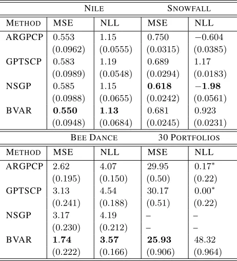
As in Saatc¸i et al. (2010), ARGPCP will refer to the non-linear GP-based AR model, GPTSCP to the time-deterministic model, and NSGP to the non-stationary GP allowing hyper-parameters to change at every CP. Saatc¸i et al. (2010) compute the mean squared error (MSE) as well as the negative log predictive likelihood (NLL) of the one-step-ahead predictions for three data sets: The water height of the Nile between622−1284AD, the snowfall in Whistler (Canada) over a 37 year period and the3-dimensional time series (x-,y-coordinate and headangle) of a honey bee dur-ing a waggle dance sequence. In Turner (2012), all of the models except NSGP were also compared on daily returns for30industry portfolios from1975−2008. In Table 1, BOCPDMS is compared to these benchmarks forM con-sisting of BAR and (SS)BVAR models.

6.1.1. DESIGNINGM

The Nile and the snowfall data are univariate, meaningM contains only BARs. For the3-dimensional bee data,M contains unrestricted BVARs and BARs. Lastly, different neighbourhood systems are built for the30Portfolio data set. Two by computing the spaces of the pairwise contem-poraneous correlations and autocorrelationspriorto1975 and using distances in these spaces, the third by using the

Standard Industrial Classification (SIC)system, withp(·) decreasing linearly.

6.1.2. FINDINGS

Table 1.Predictive MSE and NLL of BOCPDMS in comparison to GP-based techniques, with95% error bars. GP results are as reported in Saatc¸i et al. (2010) and Turner (2012). NLLs marked∗are centered in Turner (2012) so that the NLL of the best-performing GP-method amongst them is0.0.

NILE SNOWFALL

METHOD MSE NLL MSE NLL

ARGPCP 0.553 1.15 0.750 −0.604

(0.0962) (0.0555) (0.0315) (0.0385)

GPTSCP 0.583 1.19 0.689 1.17

(0.0989) (0.0548) (0.0294) (0.0183)

NSGP 0.585 1.15 0.618 −1.98

(0.0988) (0.0655) (0.0242) (0.0561)

BVAR 0.550 1.13 0.681 0.923

(0.0948) (0.0684) (0.0245) (0.0231) BEEDANCE 30 PORTFOLIOS

METHOD MSE NLL MSE NLL

ARGPCP 2.62 4.07 29.95 0.17∗

(0.195) (0.150) (0.50) (0.22)

GPTSCP 3.13 4.54 30.17 0.00∗

(0.241) (0.188) (0.51) (0.22)

NSGP 3.17 4.19 – –

(0.230) (0.212) – –

BVAR 1.74 3.57 25.93 48.32

(0.222) (0.166) (0.906) (0.964)

for hyperparameter optimization at each observation (Saatc¸i et al., 2010). Overall, there are three main reasons why BOCPDMS performs better: Firstly, being able to change lag lengths between CPs seems more important to predictive performance than being able to model non-linear dynamics. Secondly, unlike the GP-models, we allow the time series to communicate via{AL

l}. Thirdly, the hyperparameters

of the GP have a strong influence on inference. In partic-ular, the noise varianceσis treated as a hyperparameter and optimized via type-II ML. Except for the NSGP, this is only done during a training period. Thus, the GP-models cannot adapt to the observations after training, leading to overconfident predictive distributions that are too narrow (as also noted in Turner, 2012, p. 172). This in turn leads them to be more sensitive to outliers, and to mislabel them as CPs. In contrast, (10a)–(10d) modelsσas part of the infer-ential Bayesian hierarchy, and hyperparameter optimization is instead applied at one level higher. Consequently, our predictive distributions are wider, and the algorithm is less confident about the next observations, making it more ro-bust to outliers. This is also responsible for the overall smaller standard errors of the GP-models in Table 1, since the GPs interpret outliers as CPs and immediately adapt to short-term highs or lows.

CP Detection:A good demonstration of this finding is the Nile data set, where the MAP segmentation finds a sin-gle CP, corresponding to the installation of the nilometer around715CE, see Fig 5. In contrast, Saatc¸i et al. (2010) re-port18additional CPs corresponding to outliers. The same phenomenon is also reflected in the run-length distribution (RLD): While the probabilty mass in Figs. 3, 4 and 5 are spread across the retained run-lengths, the RLD reported in Saatc¸i et al. (2010) is more concentrated and even degen-erate for the30Portfolio data set. On the other hand, such enhanced sensitivity to change can be advantageous. For instance, in the bee waggle dance, the GP-based techniques are better at identifying the true CPs. The reason is twofold: Firstly, the variance for the bee waggle data is homogeneous across time, so treating it as fixed helps inference. Sec-ondly, the CPs in this data set are subtle, so having narrower predictive distributions is of great help in detecting them. However, it adversely affects performance when changes in the error variance are essential, as for financial data: In particular, BOCPDMS finds the ground truths labelled in Saatc¸i et al. (2010), and discovers even more, see Fig. 3. This is especially apparent in times of market turmoil where changes in the variance of returns are significant. We show this using the example of the subprime mortgage financial crisis: While the RLD of Saatc¸i et al. (2010) identified only 2CPs with ground truth and a third unlabelled one during the height of the crisis, BOCPDMS detects a large number of CPs corresponding to ground truths, see Fig. 4.

Lastly, we note that segmentations obtained off-line for both the bee waggle dance and the30Portfolios are reported in Xuan & Murphy (2007). Compared to the on-line segmenta-tions produced by BOCPDMS, these are closer to the truth for the bee waggle data, but not for the30Portfolio data set.

Model selection:In most of the experiments where abrupt changes model the non-stationarity well, the model posterior is fairly concentrated and periods of model uncertainty are

2 0 2

River Height

700 800 900 1000 1100 1200

Year

200 400 600

run length

nilometer

1022 ₁₀19 ₁₀16 ₁₀13 ₁₀10 ₁₀7 ₁₀4 ₁₀1

5

0

5

°C

M(5+)

M(6)

M(6+)

M(7)

M(7+)

₁

₂

₃

1880

1900

1920

1940

1960

1980

2000

Year

0

100

log(SGV)

Figure 6.Results for European Temperatures: Panel 1: normal-ized temperature for Prague and JenaPanel 2:Model Posterior maximum,mbt= arg maxM{P(mt|y1:t)}, model complexity

de-creasing top to bottom. M(l), M(l+)are SSBVAR withllags. Spatial dependence inM(l+)is slower decaying. Periods of model uncertainty are (1)2nd Industrial Revolution1870−1914, (2) Post WW2 boom1950−1973, (3) European Climate shift 1987−present, see Luterbacher et al. (2004). Panel 3: To com-pare model uncertainty across different data andM, the (Log) Standardized Generalized Variance (SGV)ofmbtcan be used.

short. This is different when changes are slower, see Fig. 6. The implicit model complexity penalization Bayesian model selection performs provides BOCPDMS with an Occam’s Razor mechanism: Simple models are typically favoured until evidence for more complex dynamics accumulates. For the bee waggle and the30Portfolio data set, BVARs are preferred to BARs. For the30Portfolio data, the MAP segmentation only selects SSBVARs with neighbourhoods constructed from contemporaneous correlation and autocor-relations. Neighbourhoods using SIC codes are not selected, reflecting that this classification from1937is out of date.

6.2. Performance on spatio-temporal data

European Temperature: Monthly temperature averages 01/01/1880−01/01/2010for the21longest-running sta-tions across Europe are taken from http://www.ecad.eu/. We adjust for seasonality by subtracting monthly averages for each station. Station longitudes and latitudes are avail-able, soN(S)is based on concentric rings around the sta-tions using Euclidean distances. Two different decay func-tionsp(·), p+(·) are used, withp+(·)using larger neigh-bourhoods and slower decaying. Temperature changes are poorly modeled by CPs and more likely to undergo slow transitions. Fig. 6 shows the way in which the model pos-terior captures such longer periods of change in dynamics. The values on the bottom panel are calculated by consid-eringm_bt= arg maxM∈MP(mt|y1:t)as|M|-dimensional

multinomial random variable. Its Standardized Generalized Variance (SGV) (Wilks, 1960; SenGupta, 1987) is

calcu-lated as|M|-th root of the covariance matrix determinant. We plot the log of the SGV computed using the model pos-teriors for the last8years. This provides an informative summary of the model posterior dispersion.

Air Pollution:Finally, we analyze Nitrogen Oxide (NOX) observed at 29 locations across London 17/08/2002 − 17/08/2003. The quarterhourly measurements are aver-aged over24hours. Weekly seasonality is accounted for by subtracting week-day averages for each station. Mis populated with SSBVAR models whose neighbourhoods are constructed from both road- and Euclidean distances. As17/02/2003marks the introduction of London’s first ever congestion charge, we find structural changes in the dynamics around that date. A model with shorter lag length but identical neighbourhood structure is preferred after the congestion charge. In Fig. 7, Bayes Factors (BFs) capture the shift: Kass & Raftery (1995) classify logs of BFs as very strong evidence if their absolute value exceeds5.

7. Conclusion

We have extended Bayesian On-line Changepoint Detection (BOCPD) to multiple models by generalizing Fearnhead & Liu (2007) and Adams & MacKay (2007), arriving at BOCPDMS. For inference in multivariate data streams, we propose BVARs with closed form distributions that have strong theoretical guarantees summarized in Thm. 1. We sparsify BVARs based on neighbourhood systems, thus mak-ing BOCPDMS especially amenable to spatio-temporal in-ference. To demonstrate the power of the resulting frame-work, we apply it to multivariate real world data, outper-forming the state of the art. In future work, we would like to add and remove models fromMon-line. This could lower the computational cost for the case where |M| is significantly larger than the number of threads.

0.0 2.5

NOX

0 1

P(m|y)

2002-09 2002-11 2003-01 2003-03 2003-05 2003-07 2003-09 100

0 100

log(BF)

Acknowledgements

JK is funded by the EPSRC grant EP/L016710/1 . Further, this work was supported by The Alan Turing Institute under EPSRC grant EP/N510129/1 as well as the Lloyds Register Foundation programme on Data Centric Engineering.

References

Adams, Ryan Prescott and MacKay, David JC. Bayesian online changepoint detection. arXiv preprint arXiv:0710.3742, 2007.

Barry, Daniel and Hartigan, John A. A bayesian analy-sis for change point problems. Journal of the American Statistical Association, 88(421):309–319, 1993.

Caron, Franc¸ois, Doucet, Arnaud, and Gottardo, Raphael. On-line changepoint detection and parameter estimation with application to genomic data.Statistics and Comput-ing, 22(2):579–595, 2012.

Fazayeli, Farideh and Banerjee, Arindam. Generalized di-rect change estimation in ising model structure. In In-ternational Conference on Machine Learning, pp. 2281– 2290, 2016.

Fearnhead, Paul. Exact bayesian curve fitting and signal segmentation. IEEE Transactions on Signal Processing, 53(6):2160–2166, 2005.

Fearnhead, Paul and Liu, Zhen. On-line inference for mul-tiple changepoint problems.Journal of the Royal Statis-tical Society: Series B (StatisStatis-tical Methodology), 69(4): 589–605, 2007.

Garnett, Roman, Osborne, Michael A, and Roberts, Stephen J. Sequential bayesian prediction in the pres-ence of changepoints. InProceedings of the 26th Annual International Conference on Machine Learning, pp. 345– 352. ACM, 2009.

Guill´en, Mauro F. The global economic & financial crisis: A timeline.The Lauder Institute, University of Pennsyl-vania, pp. 1–91, 2009.

Hannan, EJ and Kavalieris, L. Regression, autoregression models. Journal of Time Series Analysis, 7(1):27–49, 1986.

Herlands, William, Wilson, Andrew, Nickisch, Hannes, Flaxman, Seth, Neill, Daniel, Van Panhuis, Wilbert, and Xing, Eric. Scalable gaussian processes for characterizing multidimensional change surfaces. InArtificial Intelli-gence and Statistics, pp. 1013–1021, 2016.

Inoue, Akihiko and Kasahara, Yukio. Explicit representation of finite predictor coefficients and its applications. The Annals of Statistics, pp. 973–993, 2006.

Inoue, Akihiko, Kasahara, Yukio, Pourahmadi, Mohsen, et al. Baxters inequality for finite predictor coeffi-cients of multivariate long-memory stationary processes.

Bernoulli, 24(2):1202–1232, 2018.

Kass, Robert E and Raftery, Adrian E. Bayes factors. Jour-nal of the american statistical association, 90(430):773– 795, 1995.

Khaleghi, Azadeh and Ryabko, Daniil. Asymptotically consistent estimation of the number of change points in highly dependent time series. InInternational Confer-ence on Machine Learning, pp. 539–547, 2014.

Li, Shuang, Xie, Yao, Dai, Hanjun, and Song, Le. M-statistic for kernel change-point detection. InAdvances in Neural Information Processing Systems, pp. 3366–3374, 2015.

Lin, Kevin, Sharpnack, James L, Rinaldo, Alessandro, and Tibshirani, Ryan J. A sharp error analysis for the fused lasso, with application to approximate changepoint screening. InAdvances in Neural Information Process-ing Systems, pp. 6887–6896, 2017.

Liu, Song, Yamada, Makoto, Collier, Nigel, and Sugiyama, Masashi. Change-point detection in time-series data by relative density-ratio estimation. Neural Networks, 43: 72–83, 2013.

Luterbacher, J¨urg, Dietrich, Daniel, Xoplaki, Elena, Gros-jean, Martin, and Wanner, Heinz. European seasonal and annual temperature variability, trends, and extremes since 1500.Science, 303(5663):1499–1503, 2004.

Meyer, Marco and Kreiss, Jens-Peter. On the vector autore-gressive sieve bootstrap.Journal of Time Series Analysis, 36(3):377–397, 2015.

Niekum, Scott, Osentoski, Sarah, Atkeson, Christopher G, and Barto, Andrew G. Champ: Changepoint detection using approximate model parameters. Technical report, (No. CMU-RI-TR-14-10) Carnegie-Mellon University Pittsburgh PA Robotics Institute, 2014.

Saatc¸i, Yunus, Turner, Ryan D, and Rasmussen, Carl E. Gaussian process change point models. InProceedings of the 27th International Conference on Machine Learning (ICML-10), pp. 927–934, 2010.

SenGupta, Ashis. Generalizations of barlett’s and hartley’s tests of homogeneity using overall variability. Commu-nications in Statistics-Theory and Methods, 16(4):987– 996, 1987.

Turner, Ryan, Saatci, Yunus, and Rasmussen, Carl Edward. Adaptive sequential bayesian change point detection. In

Turner, Ryan D, Bottone, Steven, and Stanek, Clay J. On-line variational approximations to non-exponential family change point models: with application to radar tracking. InAdvances in Neural Information Processing Systems, pp. 306–314, 2013.

Turner, Ryan Darby. Gaussian processes for state space models and change point detection. PhD thesis, Univer-sity of Cambridge, 2012.

Wilks, SS. Multidimensional statistical scatter. Contribu-tions to probability and statistics, pp. 486–503, 1960.

Wilson, Robert C, Nassar, Matthew R, and Gold, Joshua I. Bayesian online learning of the hazard rate in change-point problems.Neural computation, 22(9):2452–2476, 2010.