Using Gaussian processes to model light curves in the presence of flickering : the eclipsing cataclysmic variable ASASSN 14ag

warwick.ac.uk/lib-publications

Original citation:

McAllister, M. J., Littlefair, S. P., Dhillon, V. S., Marsh, T. R., Ashley, R. P., Bours, Madelon C.

P., Breedt, E., Hardy, L. K., Hermes, J. J., Kengkriangkrai, S., Kerry, P., Rattanasoon, S. and

Sahman, D. I.. (2017) Using Gaussian processes to model light curves in the presence of

flickering : the eclipsing cataclysmic variable ASASSN-14ag. Monthly Notices of the Royal

Astronomical Society, 464 (2). pp. 1353-1364.

Permanent WRAP URL:

http://wrap.warwick.ac.uk/84758

Copyright and reuse:

The Warwick Research Archive Portal (WRAP) makes this work by researchers of the

University of Warwick available open access under the following conditions. Copyright ©

and all moral rights to the version of the paper presented here belong to the individual

author(s) and/or other copyright owners. To the extent reasonable and practicable the

material made available in WRAP has been checked for eligibility before being made

available.

Copies of full items can be used for personal research or study, educational, or not-for profit

purposes without prior permission or charge. Provided that the authors, title and full

bibliographic details are credited, a hyperlink and/or URL is given for the original metadata

page and the content is not changed in any way.

Publisher’s statement:

This article has been accepted for publication in Monthly Notices of the Royal Astronomical

Society © 2016 The Authors Published by Oxford University Press on behalf of the Royal

Astronomical Society. All rights reserved.

Link to final published version:

http://dx.doi.org/10.1093/mnras/stw2417

A note on versions:

The version presented in WRAP is the published version or, version of record, and may be

cited as it appears here.

Using Gaussian processes to model light curves in the presence

of flickering: the eclipsing cataclysmic variable ASASSN-14ag

M. J. McAllister,

S. P. Littlefair,

V. S. Dhillon,

T. R. Marsh,

R. P. Ashley,

M. C. P. Bours,

E. Breedt,

L. K. Hardy,

J. J. Hermes,

S. Kengkriangkrai,

P. Kerry,

S. Rattanasoon

and D. I. Sahman

1_{Department of Physics and Astronomy, University of Sheffield, Sheffield S3 7RH, UK} 2_{Instituto de Astrofisica de Canarias, E-38205 La Laguna, Tenerife, Spain}

3_{Department of Physics, University of Warwick, Coventry CV4 7AL, UK}

4_{Departmento de F´ısica y Astronom´ıa, Universidad de Valpara´ıso, Avenida Gran Bretana 1111, Valpara´ıso 2360102, Chile} 5_{Department of Physics, University of North Carolina, Chapel Hill, NC 27599, USA}

6_{National Astronomical Research Institute of Thailand, 191 Siriphanich Building, Huay Kaew Road, Chiang Mai 50200, Thailand}

Accepted 2016 September 22. Received 2016 September 19; in original form 2016 August 3

A B S T R A C T

The majority of cataclysmic variable (CV) stars contain a stochastic noise component in their light curves, commonly referred to as flickering. This can significantly affect the morphology of CV eclipses and increases the difficulty in obtaining accurate system parameters with reliable errors through eclipse modelling. Here we introduce a new approach to eclipse modelling, which models CV flickering with the help of Gaussian processes (GPs). A parametrized eclipse model – with an additional GP component – is simultaneously fitted to eight eclipses of the dwarf nova ASASSN-14ag and system parameters determined. We obtain a mass ratio

q=0.149±0.016 and inclinationi=83.◦4₋+0₀◦◦._.9₆. The white dwarf and donor masses were found to beMw=0.63±0.04 MandMd=0.093+₋00..015012M, respectively. A white dwarf

temperature Tw =14 000 +₋22002000 K and distance d =146 +−2420 pc were determined through

multicolour photometry. We find GPs to be an effective way of modelling flickering in CV light curves and plan to use this new eclipse modelling approach going forward.

Key words: methods: data analysis – binaries: close – binaries: eclipsing – stars: dwarf novae – stars: individual: ASASSN-14ag.

1 I N T R O D U C T I O N

Cataclysmic variable (CV) stars are interacting binary systems that contain a white dwarf primary and a low-mass secondary. Material from the secondary star is transferred to the white dwarf due to the secondary filling its Roche lobe. If the white dwarf has a low mag-netic field, this transferred mass does not immediately accrete on to the white dwarf. Instead, in order to conserve angular momentum, the transferred mass forms an accretion disc around the white dwarf. A bright spot is formed at the point on the accretion disc where the gas stream from the donor makes contact. For a general review of CVs, see Hellier (2001).

At high enough inclinations to our line of sight (>80◦), the donor star can eclipse all other components within the system. As this includes the white dwarf, accretion disc and bright spot, CV eclipses

_{E-mail:[email protected]}

†_{Hubble Fellow.}

can appear complex in shape. All of these components are eclipsed in quick succession, therefore high time resolution photometry is required to reveal all the individual eclipse features. Measuring the timings of the white dwarf and bright spot eclipse features allows the system parameters to be accurately determined (e.g. Wood et al.

1986).

For some systems, the timing of these features (especially those associated with the bright spot) cannot be accurately measured, even with high time resolution. This can be due to such systems containing a high amount of flickering, seen as random variability in CV light curves with amplitudes reaching the same order of magnitude as the bright spot eclipse features. Flickering in CVs is found to originate in both the bright spot and the inner accretion disc, and is due to the turbulent nature of the transferred material within the system (Bruch2000,2015; Baptista & Bortoletto2004; Scaringi et al.2012; Scaringi2014).

Previous photometric studies of eclipsing CVs have used the averaging of multiple eclipses as a way of overcoming flickering and strengthening the bright spot eclipse features, before fitting an

at University of Warwick on January 9, 2017

http://mnras.oxfordjournals.org/

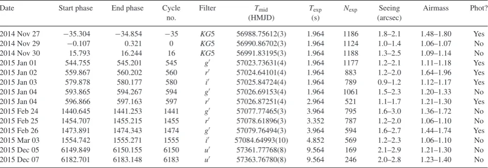
Table 1. Journal of observations. The dead time between exposures was 0.015 s for all observations. The relative timestamping accuracy is of the order of

10µs, while the absolute GPS timestamp on each data point is accurate to<1 ms.Tmidrepresents the mid-eclipse time, whileTexpandNexprepresent the

exposure time and number of exposures, respectively. The last column indicates whether or not the conditions were photometric.

Date Start phase End phase Cycle Filter Tmid Texp Nexp Seeing Airmass Phot?

no. (HMJD) (s) (arcsec)

2014 Nov 27 −35.304 −34.854 −35 KG5 56988.75612(3) 1.964 1186 1.8–2.1 1.48–1.80 Yes

2014 Nov 29 −0.107 0.321 0 KG5 56990.86702(3) 1.964 1124 1.0–1.4 1.06–1.07 No

2014 Nov 30 15.793 16.244 16 KG5 56991.83195(3) 1.964 1188 1.3–2.5 1.09–1.14 No

2015 Jan 01 544.755 545.201 545 g 57023.73631(4) 1.964 1177 1.2–2.1 1.11–1.18 Yes

2015 Jan 02 559.867 560.202 560 r 57024.64101(4) 1.964 883 1.2–2.0 1.64–1.96 Yes

2015 Jan 03 579.878 580.177 580 i 57025.84724(4) 1.964 789 0.9–1.2 1.12–1.17 Yes

2015 Jan 04 593.865 594.267 594 g 57026.69153(4) 1.964 1061 1.5–2.3 1.20–1.33 No

2015 Jan 04 596.866 597.163 597 r 57026.87251(4) 2.964 521 1.1–1.7 1.21–1.30 Yes

2015 Feb 24 1440.645 1441.253 1441 g 57077.77465(3) 3.964 795 1.6–3.0 1.36–1.72 No

2015 Feb 25 1454.707 1455.215 1455 r 57078.61896(3) 3.352 787 1.2–2.0 1.06–1.10 No

2015 Feb 26 1473.891 1474.343 1474 g 57079.76494(3) 3.964 594 1.6–2.7 1.44–1.74 Yes

2015 Mar 03 1554.742 1555.271 1555 i 57084.64993(10) 4.852 569 1.2–2.3 1.06–1.10 No

2015 Dec 05 6149.849 6150.155 6150 u 57361.77768(8) 9.564 169 2.1–2.9 1.21–1.30 No

2015 Dec 07 6182.701 6183.148 6183 u 57363.76780(8) 9.564 246 2.0–2.8 1.23–1.40 No

eclipse model to obtain system parameters (e.g. Savoury et al.2011; Littlefair et al.2014; McAllister et al.2015). McAllister et al. (2015) also attempted to estimate the effect of flickering on the parameter uncertainties. An additional four g-band eclipses were created – each containing a different combination of three out of the four original eclipses used for theg-band average – and fitted separately. The spread in system parameters from these average eclipses gave an indication of the error due to flickering, approximately five times the size of the purely statistical error.

A downside to the eclipse averaging approach concerns the in-consistent bright spot ingress/egress positions due to changes in the accretion disc radius, which are observed in a significant num-ber of systems. Averaging such light curves can lead to inaccurate bright spot eclipse timings and therefore incorrect system param-eters. Eclipse light curves from systems with disc radius changes have to be fitted individually, requiring another method to combat flickering. Here we introduce a new approach, involving the mod-elling of flickering in individual eclipses with the help of Gaussian processes (GPs).

GPs have been used for many years in the machine learning com-munity (see textbooks Bishop2006; Rasmussen & Williams2006) and have recently started seeing use in many areas of astrophysics. Some examples include photometric redshift prediction (Way & Srivastava2006; Way et al.2009), modelling instrumental system-atics in transmission spectroscopy (Gibson et al.2012; Evans et al.

2015) and modelling stellar activity signals in radial velocity studies (Rajpaul et al.2015). See Section 3 for further discussion of GPs.

The modelling of flickering is just one of the number of mod-ifications we have made to the fitting approach. The model now has the ability to fit multiple eclipses simultaneously, whilst sharing parameters intrinsic to a particular system, e.g. mass ratio (q), white dwarf eclipse phase full width at half-depth (φ) and white dwarf radius (Rw) between all eclipses. More details on the modifications of the model can be found in Section 4.3.

ASASSN-14ag was the chosen system to test the new modelling approach due to the combination of a high level of flickering and clear bright spot features in its eclipse light curves. ASASSN-14ag was discovered in outburst (reaching V = 13.5) by the All-Sky Automated Search for Supernovae (ASAS-SN; Shappee et al.2014) on 2014 March 14. A look through existing light-curve data on this system from the Catalina Real-Time Survey (CRTS; Drake

et al.2009) showed signs of eclipses, with an orbital period below the period gap (vsnet-alert 17036). Follow-up photometry made in the days following the initial ASAS-SN discovery confirmed the eclipsing nature of the CV (vsnet-alert 17041). The discovery of superhumps also showed this to be a superoutburst, identifying ASASSN-14ag as an SU UMa-type dwarf nova (vsnet-alert 17042; Kato et al.2015).

2 O B S E RVAT I O N S

ASASSN-14ag was observed a total of 14 times from 2014 Nov to 2015 Dec using the high-speed single beam camera ULTRASPEC (Dhillon et al.2014) on the 2.4 m Thai National Telescope (TNT), Thailand. Eclipses were observed in the SDSSugriand Schott

KG5 filters. The SchottKG5 filter is a broad filter, covering approx-imatelyu+g+r. A complete journal of observations is shown in Table1.

Data reduction was carried out using the ULTRACAM pipeline reduction software (see Feline et al.2004). A nearby, bright and photometrically stable comparison star was used to correct for any transparency variations during observations.

The standard stars SA 92-288 (observed on 2015 Jan 1), SA 97-249 (2015 Jan 2), SA 93-333 (2015 Jan 3 & 2015 Dec 11), SA 97-351 (2015 Mar 3) and SA 100-280 (2015 Dec 10) were used to transform the photometry into theugrizstandard system (Smith et al.2002). TheKG5 filter was calibrated using a similar method to Bell et al. (2012); see appendix of Hardy et al. (2016, submitted) for a full description of the calibration process. AKG5 magnitude was calculated for the SDSS standard star SA 97-249 (2015 Feb 27) and used to find a target flux in theKG5 band. Photometry was corrected for atmospheric extinction using extinction values – for all bands – measured at the observatory (Dhillon et al.2014).

3 G AU S S I A N P R O C E S S E S

Our aim here is to only briefly cover the topic of GPs as they are covered extensively elsewhere in the literature. We recommend the textbooks of Rasmussen & Williams (2006) and Bishop (2006) as general overviews of the topic, while useful introductions to the use of GPs for modelling time series data can be found in Roberts et al. (2013) and the appendix of Gibson et al. (2012).

at University of Warwick on January 9, 2017

http://mnras.oxfordjournals.org/

In the same way, a single data point can be represented by a Gaussian random variable, and a light curve of observablesycan be represented by a multivariate Gaussian distribution, which is completely specified by the mean values,μ, and a covariance matrix,

K. Trends in the light curve are captured by correlations between nearby data points, i.e. off-diagonal entries in the covariance matrix. The covariance matrix is represented by

Kij =σi2δij+k(ti, tj) (1)

consisting of a white noise component, σ2

iδij, and a covariance function,k(ti,tj). The covariance function determines the

covari-ance between any two data points and is chosen to best represent the stochastic process to be modelled. For modelling flickering in CV light curves, the Mat´ern-3/2 kernel was favoured over the more commonly used squared-exponential kernel. This is due to the Mat´ern-3/2’s greater ability at recreating the sharp features of flickering that comes from being finitely differentiable. The Mat´ern-3/2 kernel has the following form:

k(t_i, t_j)=h2

1+√3|ti−tj| λ

exp

−√3|ti−tj| λ

, (2)

wherek(ti, tj) is theijth element of kand ti andtjrepresent the

times of any two data points (Roberts et al.2013). Bothhandλ arehyperparametersof the GP, and they control the output scale (amplitude) and the input scale (time), respectively. Once a kernel function has been constructed, it is straightforward to calculate the likelihood,L, of a data set:

logL_μ,k(h, λ)= −1 2r

T_K−1

r − 1

2log|K| − n

2log(2π) (3)

wherer= y−μrepresents the vector of the residuals after sub-traction of the mean function,μ, from the data, y, and nis the number of data points (Rasmussen & Williams2006). The mean and uncertainty of the GP can also be calculated given observed data, i.e. the posterior mean and uncertainty (see equations 8 and 9 in Roberts et al.2013). Equation (3) is expensive to compute due to the need for inverting theN×Ncovariance matrix, requiringO(n3₎ operations. For large matrices, it is possible to speed up this step by using an alternative solver based on anO(nlog2_{n) algorithm for} inversion (Ambikasaran et al.2014).

As mentioned in Section 1, there are multiple sources of flick-ering in CVs, and therefore more than one flickflick-ering amplitude. The observed amplitude should vary across the eclipse as the differ-ent compondiffer-ents are individually eclipsed. GPs are stationary, and therefore act the same across all points in the time series. To ac-commodate for the anticipated changes in flickering amplitude, two

changepointswere introduced. These changepoints are positioned at the white dwarf’s ingress start,tin, and egress end,te. This en-abled the kernel function amplitude hyperparameter outside white dwarf eclipse,h1, to differ from that inside,h2. The location of the changepoints was chosen on the basis that the inner disc is a main source of flickering, but not the only source. The input scale hyperparameter was kept the same across the whole time series. The drastic changepoint approach from Garnett et al. (2010) was implemented, with the kernel function taking the following form:

k(t1, t2;h1, h2) ⎧ ⎪ ⎪ ⎪ ⎨ ⎪ ⎪ ⎪ ⎩

k(t1, t2;h1), t1, t2< tin k(t1, t2;h2), t1, t2≥tin;t1, t2≤te k(t1, t2;h1), t1, t2> te

0, otherwise.

(4)

Figure 1. All 12 ASASSN-14ag eclipses that are not badly affected by atmospheric conditions. Each plot contains those eclipses observed in one of the five wavelength bands, with the name of each band in the bottom-right corner of each plot.

4 R E S U LT S

4.1 Orbital ephemeris

Mid-eclipse times (Tmid) were determined assuming that the white dwarf eclipse is symmetric around phase zero:Tmid=(Twi+Twe)/2, whereTwi andTweare the times of white dwarf mid-ingress and mid-egress, respectively.TwiandTwewere determined by locating the minimum and maximum times of the smoothed light-curve derivative. The Tmid errors (see Table 1) were adjusted to give χ2_{=1 with respect to a linear fit.}

All eclipses were used to determine the following ephemeris:

HMJD=56990.867004(12)+0.060310665(9)E.

This ephemeris was used to phase fold the data for the analysis that follows.

4.2 Light-curve morphology and variations

Fig.1shows 12 of the 14 total ASASSN-14ag eclipses. The eclipses of 2015 March 3 and 2015 December 5 were affected by poor at-mospheric conditions, so were not used in this study. The eclipses in Fig.1all have a clear white dwarf eclipse feature (phase−0.03 to 0.03), and the majority also have a discernible bright spot eclipse feature (phase−0.02 to 0.08). The positions of bright spot ingress

at University of Warwick on January 9, 2017

http://mnras.oxfordjournals.org/

and egress appear to occur at slightly different phases in each eclipse. This may be evidence for small changes in the accre-tion disc radius or could be due to flickering, which is inherent to every eclipse and of varying amplitude from one eclipse to the next.

The majority of the flickering occurs outside of white dwarf eclipse. In some cases, it re-appears almost immediately after white dwarf egress, implying the source of flickering to be in proximity to the white dwarf, perhaps in either the inner disc or the boundary layer. In a number of eclipses, there is a small amount of flicker-ing visible between the two flicker-ingress features. As the white dwarf is eclipsed during this period, there must be another source of flicker-ing within the system. Flickerflicker-ing is greatly reduced once both the white dwarf and bright spot are eclipsed, which points to the bright spot as the secondary source of flickering.

The highest amplitude flickering is seen in the three eclipses that were observed while the system was in a slightly higher photometric state, with one such eclipse in each of theKG5,g andr bands (Fig.1). The higher photometric state is most likely to be the result of a more luminous disc. The high stategandrband eclipses do show a clear bright spot egress feature, but an ingress is not visible in any of the three eclipses and therefore none were included for model fitting.

4.3 Modifications to existing model

The model of the binary system used to calculate eclipse light curves contains contributions from the white dwarf, bright spot, accretion disc and secondary star, and is described in detail by Savoury et al. (2011). The model requires a number of assumptions, including that of an unobscured white dwarf (Savoury et al.2011). As stated in McAllister et al. (2015), we feel this is still a reasonable assumption to make despite the validity of the assumption being questioned by Spark & O’Donoghue (2015) through fast photometry observations of the dwarf nova OY Car.

We have made modifications to this model so that it is now possible to fit multiple eclipse light curves simultaneously, with theq,Rw/aandφparameters shared between all eclipses. Each eclipse in the simultaneous fit also has either 11 or 15 (depending on whether the simple or complex bright spot model is used; Savoury et al.2011) parameters that are unique to that eclipse. Due to the prominence of the bright spot in ASASSN-14ag, the complex bright spot model was used in all fits. The three shared parameters, once constrained through model fitting, can then be used to calculate system parameters (see Section 4.4.2).

With GPs included to model the flickering, the total number of model parameters are increased by three with the inclusion of the three kernel function hyperparameters (see Section 3). When fitting the eclipse model, the flickering is handled by using the residuals – obtained by subtracting the eclipse model from the data – to calculate the model likelihood using equation (3).

4.4 Simultaneous light-curve modelling

Discarding the two eclipses affected by poor atmospheric condi-tions and the three eclipses in the higher photometric state left a total of nine eclipses to be used for modelling. The eight of these eclipses taken in bands other thanu were simultaneously fitted with the model, both with and without the use of GPs. Theu-band eclipse was not used in the simultaneous fit as a consequence of its lower signal to noise and time resolution compared to other wave-length bands, although it was fitted separately (see below). All 123

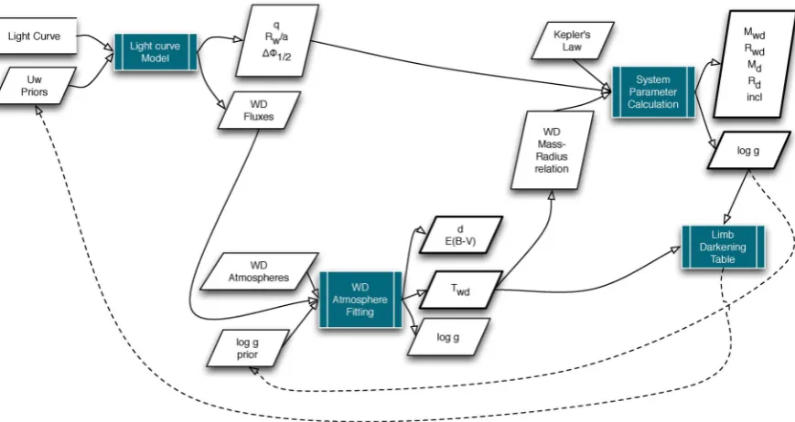
parameters (126 in the GP case) were left to fit freely except the eight limb-darkening parameters (Uw). This is due to our data not being of sufficient cadence and signal to noise to enable the shape of the white dwarf ingress/egress features to be determined, a re-quirement forUwto be accurately constrained. TheUwparameter’s priors were heavily constrained around values determined from a preliminary run through the fitting procedure described below and shown schematically in Fig.2.

A parallel-tempered Markov chain Monte Carlo (MCMC) en-semble sampler (Earl & Deem2005; Foreman-Mackey et al.2013) was used to draw samples from the posterior probability distribution of the model parameters. A parallel-tempered sampler was chosen due to the large number of model parameters to be fitted, and there-fore the large size of parameter space. Parallel-tempering involves multiple MCMCs running simultaneously, all at different ‘temper-atures’,T. Each MCMC samples from a modified posterior:

πT(x)=[l(x)]1/Tp(x), (5)

wherel(x) andp(x) represent the likelihood and prior functions, re-spectively. As equation (5) shows, each MCMC’s likelihood func-tion scales to the power of the temperature’s reciprocal, so chains at higher temperatures can explore parameter space much more effectively. Communication between each MCMC occurs through chains at adjacent temperatures periodically swapping members of their ensemble (Earl & Deem2005). This greatly assists conver-gence to a global solution. A total of 10 MCMCs – the first of temperature one and all others a factor of√2 higher than the one before – were ran for 7500 steps. The first 5000 of these steps took the form of a burn-in phase and were discarded. Only the MCMC with a temperature equal to one at the end of the fit was used to produce the model parameter posterior probability distributions. The Gelman–Rubin diagnostic was used to confirm convergence (Gelman & Rubin1992).

4.4.1 White dwarf atmosphere fitting

Estimates of the white dwarf temperature, loggand distance were obtained through fitting white dwarf fluxes – atu,g,r,iandKG5 wavelengths – to white dwarf atmosphere predictions (Bergeron, Wesemael & Beauchamp1995) with an affine-invariant MCMC en-semble sampler (Goodman & Weare2010; Foreman-Mackey et al.

2013). Reddening was also included as a parameter, in order for its uncertainty to be taken into account, but is not constrained by our data. Its prior covered the range from 0 to the maximum galactic extinction along the line of sight (Schlafly & Finkbeiner2011). The

g,r,i &KG5 white dwarf fluxes and errors were taken as me-dian values and standard deviations from a random sample of the simultaneous eight-eclipse fit chain. Theu-band flux was obtained through an individual fit to the 2016 December 7u-band eclipse, keepingq,Rw/aandφparameters close to their values from the simultaneous fit with Gaussian priors. A 3 per cent systematic error was added to the fluxes to account for uncertainties in photometric calibration.

Knowledge of the white dwarf temperature and log g values enabled the estimation of theUwparameters, with use of the data tables in Gianninas et al. (2013). Linear limb-darkening parameters of 0.427, 0.369, 0.317 and 0.272 were determined for u, g, r

andibands, respectively. A value of 0.360 for theKG5 band was calculated by taking a weighted mean of theu,g andr values, based on the fraction of theKG5 bandpass covered by each of the three SDSS filters.

at University of Warwick on January 9, 2017

http://mnras.oxfordjournals.org/

Figure 2. A schematic of the eclipse fitting procedure used to obtain system parameters. Two iterations of the fitting procedure occur, the dotted lines show steps to be taken only during the first iteration.

4.4.2 System parameters

The posterior probability distributions of q, φ and Rw/a re-turned by the MCMC eclipse fit described in Section 4.4 were used along with Kepler’s third law, the system’s orbital period and a temperature-corrected white dwarf mass–radius relationship (Wood

1995) to calculate the posterior probability distributions of the sys-tem parameters (Savoury et al.2011), which include

(i) mass ratio,q;

(ii) white dwarf mass,Mw; (iii) white dwarf radius,Rw; (iv) white dwarf logg; (v) donor mass,Md; (vi) donor radius,Rd; (vii) binary separation,a;

(viii) white dwarf radial velocity,Kw; (ix) donor radial velocity,Kd; (x) inclination,i.

The most likely value of each distribution is taken as the value of each system parameter with upper and lower bounds derived from 67 per cent confidence levels.

The system parameters were calculated twice in total. The value for loggreturned from the first calculation was used to constrain the loggprior in a second MCMC fitting the white dwarf fluxes to model atmosphere predictions (Bergeron et al.1995) as described in Section 4.4.1. All of these steps are shown schematically in Fig.2. Constraining logghad little effect on the white dwarf temperature in this instance, although it significantly helped the distance estimate, which was very poorly constrained after the first fit.

4.4.3 Without GPs

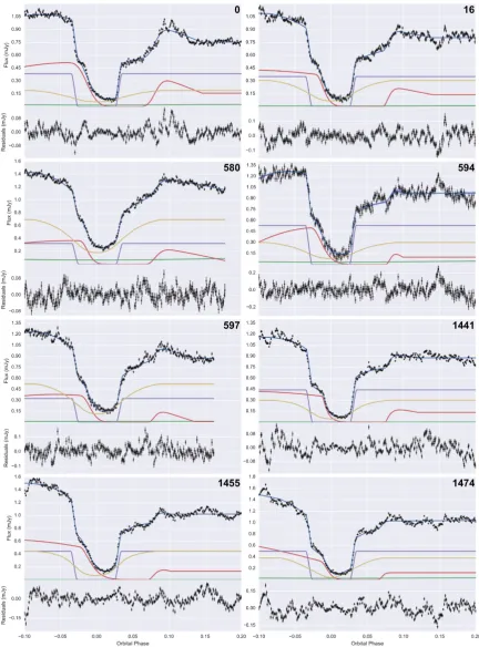
The model fit to eight eclipses simultaneously without the use of GPs is shown in Fig.3(a). The most probable fit to the eight eclipses

has aχ2_{of 17 363 with 2598 degrees of freedom. This large value} ofχ2_{is due to the large amount of flickering present in each eclipse.} The model appears to fit every white dwarf eclipse reasonably well, although there are one or two cases (e.g. cycle nos. 1441 and 1474) where the depth of the white dwarf eclipse has been overestimated slightly. In general, the bright spot eclipses have also been fitted fairly well. The major exception to this is cycle no. 0. This eclipse contains low-amplitude flickering until a slight brightening prior to bright spot egress and then a significant flicker just afterwards cov-ering the orbital phases 0.08–0.13. These two features, especially the large flicker, make it impossible for the model to correctly fit the bright spot egress. This flicker is modelled as part of the eclipse structure, at the expense of bright spot ingress, which is free from flickering but poorly fitted to accommodate for egress. Another no-table bright spot ingress misfitting is in cycle no. 1455. The ingress feature is not as clear as in other eclipses, and the nature of the flickering before the eclipse results in a falsely high bright spot flux, hindering bright spot ingress fitting. Overall, the model fits to every eclipse have been affected by flickering to some degree.

Also plotted in Fig.3(a) is a fill-between region representing 1σ from the mean of a random sample (size 1000) of the MCMC chain. In all but one case, this fill-between region is not visible due to it being thinner than the blue line of the most probable model fit. The exception to this is cycle no. 594, where it is visible just after bright spot egress (phase∼0.08). The very small distribution from a sam-ple in the chain indicates a precise solution, and this is reflected in the very small errors associated with the model parameters returned by the fit.

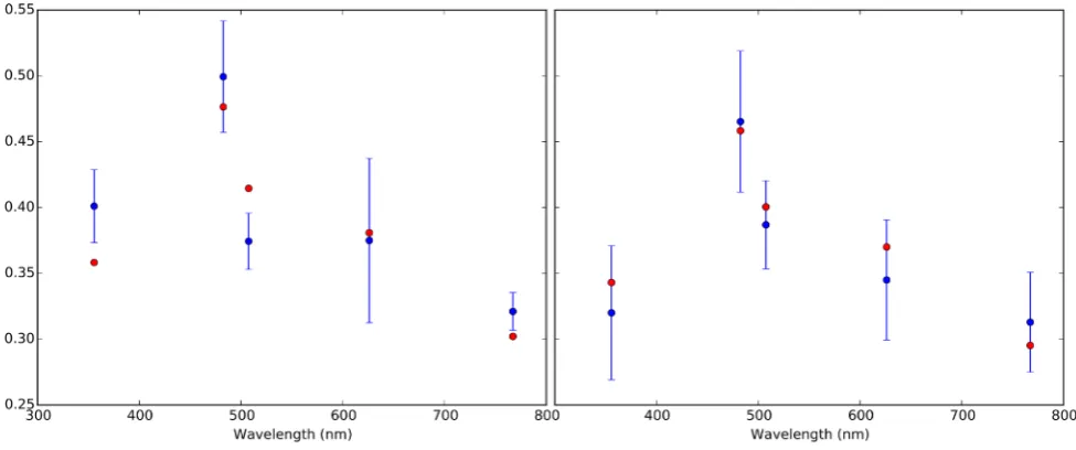
A comparison between the measured white dwarf fluxes and models can be found in the left-hand plot of Fig.4. The majority of the points calculated from the white dwarf atmosphere predictions lie outside the flux error bars, evidence for the underestimation of flux errors by the eclipse model due to flickering.

The posterior probability distributions for each system parameter are displayed in red in Fig.5, with their peak values and associated

at University of Warwick on January 9, 2017

http://mnras.oxfordjournals.org/

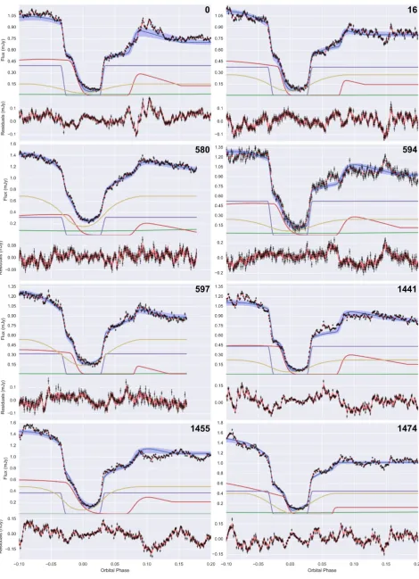
Figure 3. (a) Simultaneous model fit (blue) to eight ASASSN-14ag eclipses (black) without GPs. The blue fill-between region represents 1σ from the mean of a random sample (size 1000) of the MCMC chain, although this is thinner than the model fit line in all but one case (cycle no. 594). Also shown are the different components of the model: white dwarf (purple), bright spot (red), accretion disc (yellow) and donor (green). The residuals are shown at the bottom of each plot. Cycle numbers are displayed at the top-right corner of each plot. (b) Simultaneous model fit (blue) to eight ASASSN-14ag eclipses (black) with

GPs included. The blue fill-between region represents 1σfrom the mean of a random sample (size 1000) of the MCMC chain. The red dashed line shows the

sum of the eclipse model + posterior mean of the GP. Also shown are the different components of the model: white dwarf (purple), bright spot (red), accretion

disc (yellow) and donor (green). The residuals are shown at the bottom of each plot with the red fill-between region covering 2σfrom the posterior mean of

the GP. Cycle numbers are displayed at the top-right corner of each plot.

at University of Warwick on January 9, 2017

http://mnras.oxfordjournals.org/

Figure 3 – continued

at University of Warwick on January 9, 2017

http://mnras.oxfordjournals.org/

Figure 4. White dwarf fluxes from both simultaneous eight-eclipse and individualu-band model fits (blue) and Bergeron et al. (1995) white dwarf atmosphere

predictions (red) at wavelengths corresponding to (from left to right)u,g,KG5,randifilters. The left plot is without GPs and the right plot is with GPs.

Figure 5. Normalized posterior probability density functions for both si-multaneous eight-eclipse fits: without GPs (red) and with GPs (blue). Also included (green) are the parameter distributions calculated from the average eclipse fits (see Section 4.5).

errors – as well as temperature and distance estimates – given in the second column of Table2. The probability distributions are very narrow, which translate to small errors on the system parameters.

4.4.4 With GPs

Another set of simultaneous model fits to the eight eclipses – this time with GPs included – is shown in Fig.3(b). The most probable fit has a much higherχ2_{of 31 812 (with 2595 degrees of freedom),} reflected in the greater amplitude residuals in Fig.3(b). This is due to the additional GP component included in the fit, which models the residuals from the eclipse model fit but is not taken into account when calculating χ2_{. The GP is best visualized as the red} fill-between region covering 2σ from the GP’s posterior mean that overlays the residuals below each eclipse in Fig.3(b). The majority of residuals are covered by this fill-between region, which indicates that the chosen Mat´ern-3/2 kernel provides a good description of

Table 2. System parameters for ASASSN-14ag through simultaneous

fit-ting of eight individual eclipses, with and without the use of GPs.Twandd

represent the temperature and distance of the white dwarf, respectively.

Parameter Without GPs With GPs

q 0.1480+₋0₀._.0023₀₀₁₄ 0.149±0.016

Mw(M) 0.609+₋00..012010 0.63±0.04

Rw(R) 0.012 94+₋00..000 15000 17 0.0126±0.0006

Md(M) 0.0903₋+00..00230020 0.093+−00..015012

Rd(R) 0.1331±0.0011 0.135±0.007

a(R) 0.575±0.004 0.583±0.015

Kw(km s−1) 61.9±0.9 63±7

Kd(km s−1) 417.1+₋22..63 422±9

i(◦) 83.63₋+0_0..08₁₁ 83.4+₋0₀._.9₆

logg 7.999±0.013 8.04±0.05

Tw(K) 14 400+₋12001300 14 000+

2200

−2000

d(pc) 150+₋14₁₂ 146+₋22₁₈

CV flickering. Another representation of the GP takes the form of the sum of the eclipse model and the mean of the GP, shown by a red dashed line on the main eclipse plots.

The most obvious difference with GPs is the significantly in-creased size of the blue fill-between region in each eclipse. As mentioned in Section 4.4.3, this represents 1σfrom the mean of a random sample (size 1000) of the MCMC chain. The increase inσ is due to the much broader model parameter solution distributions, which is a consequence of fitting the model in accordance with GPs. A wider range of parameters are allowed by the data, as differences between the eclipse model and the data can be accommodated by the GP.

In contrast to the standard model fitting, it is the fill-between region, not the most probable fit, that is of most importance. In most cases, this region is in agreement with both the white dwarf and bright spot eclipse features. Cycle no. 0 is a good example to show what the GPs have brought to the model fitting. With just the eclipse model, the large flicker after bright spot egress created a very extended bright spot that could not successfully fit bright spot

at University of Warwick on January 9, 2017

http://mnras.oxfordjournals.org/

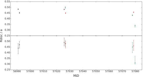
Figure 6. Accretion disc radius (Rdisc) as a fraction of the binary separation (a) versus time (in MJD) for the eight eclipses fitted simultaneously. The top

panel shows radii from the non-GP fit, while the bottom panel shows radii from the GP fit. The colour of each data point shows the wavelength band its eclipse

was observed in:KG5 (black),g(green),r(red), andi(dark red).

ingress (Fig.3a). When GPs are used, the flicker can be modelled, allowing a much more compact bright spot and a correctly fit ingress. As discussed in Section 3, our GP framework includes change-points at the start and end of white dwarf eclipse due to the expecta-tion that the amplitude of flickering should differ inside and outside white dwarf eclipse. The GP amplitude inside white dwarf eclipse returned by the fit is an order of magnitude lower compared to that outside, validating the use of changepoints.

The white dwarf atmosphere prediction fit to white dwarf fluxes obtained using GPs is shown in the right-hand plot of Fig.4. This is much improved compared to the previous fit (the left-hand side of the same figure). Comparing the white dwarf fluxes from both the standard model and GP approaches, the only flux value to have changed significantly is that of theuband. A more realisticu-band flux is obtained when fitting with GPs, as well as more representative errors in all bands.

The posterior probability distributions for each system parameter are shown in blue in Fig.5. The most likely parameter values and associated errors – as well as temperature and distance estimates – are shown in Table2. It is very evident from Fig.5that, while the distributions from each fitting approach have similar peak values, they have very contrasting values ofσ. This was already apparent from the differing sizes of the blue fill-between regions in Figs3(a) and (b), and results in the errors on the system parameters from the GP fit being significantly greater than those from the standard model fit.

4.4.5 Accretion disc

One of the parameters included in the model is the radius of the accretion disc as a fraction of the binary separation (Rdisc/a). This value from the model is actually the bright spot’s distance from the

white dwarf as a fraction of the binary separation, but we assume the bright spot to lie at the edge of the accretion disc. Plotting these values from multiple eclipses against the MJD of each eclipse – e.g. fig. 7 in McAllister et al. (2015) – enables disc radius evolution to be investigated. Fig.6showsRdisc/aagainst MJD for the eight eclipses fitted simultaneously, both without (top) and with GPs (bottom). These eclipses were observed during the same observing season, but over three separate observing runs, explaining the large gaps in Fig.6. The errors on the disc radii from the GP case are much larger than those from the non-GP case, which is expected as the errors from the non-GP case are significantly underestimated due to not taking the effects of flickering into account. Across the first two observing runs, there is very little change in disc radius. This is still the case even when the first two eclipses from the third observing run are included, but not once the final of the eight eclipses is considered. The top plot of Fig.6appears to show a significant decrease in the disc radius of the order of 0.1Rdisc/a

between the final two eclipses, separated by approximately 1 d (19 orbital cycles). With GPs included (bottom plot), this apparent decrease in the disc radius is shown to most likely be just a product of flickering, with less than a 2σ difference between the final two disc radii.

4.5 Average light-curve modelling

Previous eclipse modelling studies have used the technique of av-eraging eclipses together as a way of negating flickering and/or boosting signal to noise (Littlefair et al.2008; Savoury et al.2011; McAllister et al.2015). To investigate how this technique compares to our new approach, the individual ASASSN-14ag eclipses were used to create average eclipses, which were then fitted separately without the use of GPs. In addition, the eight individual eclipses

at University of Warwick on January 9, 2017

http://mnras.oxfordjournals.org/

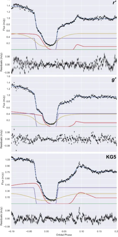
Figure 7. Model fits (blue) to average r, g andKG5 eclipses (black) without the use of GPs. Also shown are the different components of the model: white dwarf (purple), bright spot (red), accretion disc (yellow) and donor (green). The residuals are shown at the bottom of each plot.

were also fitted separately, with their spread in system parameters an indication of the effects of flickering.

The twoKG5 band eclipses (cycle nos. 0 and 16) were averaged to create aKG5 average eclipse, similarly for both theg(cycle nos. 594, 1441 and 1474) andr(cycle nos. 597 and 1455) bands (Fig.7). Due to high-amplitude flickering and the small number of eclipses, averaging is relatively ineffective in this case, with all three average eclipses containing large amounts of residual flickering. Despite this, they do all show bright spot features. The three average eclipses were individually fitted with the eclipse model (without GPs) and the resulting fits are shown in Fig.7. The system parameters for each band can be found in the first three columns of Table3, with the final column in Table3showing the weighted mean of the parameters

from each wavelength band. The errors on the parameter values in this final column are the weighted standard deviation of the parameters from fitting the eight individual eclipses separately. The system parameter distributions from the average eclipse fitting are also shown in Fig.5. A similar – though not identical – approach to estimating the error due to flickering was used in McAllister et al. (2015).

5 D I S C U S S I O N

As mentioned in Section 4.5, averaging eclipses in this particu-lar case is not an effective way of reducing flickering, as a particu-large amount of it still remains. Obtaining many more eclipses would help, but negating the flickering would not be possible due to its high-amplitude nature. This issue – coupled with the fact that many systems show disc radius changes – shows the need for a different approach to modelling CV light curves containing flickering. The approach we present here involves including flickering in the model, while fitting individual eclipses simultaneously.

5.1 Modelling of flickering

In McAllister et al. (2015), the effects of flickering were estimated looking at the spread in system parameters after fitting a further four average eclipses, each containing a different combination of three out of the four original eclipses used for theg-band average. Here, we use the spread in system parameters from fitting the eight individual eclipses separately as an estimation of flickering. The resulting system parameters are shown in Table3. These individual eclipse fits show a wide spread in system parameters, which results in large errors.

Using the new technique of modelling flickering with GPs, the error introduced by flickering no longer has to be estimated as it is already included in the errors on the system parameters returned by the model. In the case of ASASSN-14ag, the contribution from flick-ering is seen through comparison of the errors in the two columns of Table2and the difference in the red and blue distributions in Fig.5.

The size of the error introduced by flickering differs depending on whether the old or new approach is used (blue and green distri-butions in Fig.5), but which comes closest to representing the true effect? Does the old approach of using the distribution in system parameters from individual fits overestimate the error due to flicker-ing, or does the new approach of modelling flickering underestimate it?

Fig.3(b) shows that the GPs have done a good job of modelling the flickering. Therefore, the error on the model parameters – which are marginalized over the GP hyperparameters – are likely to be accurate. This suggests that the old approach of using the standard deviation of system parameters from fitting individual eclipses may overestimate the error due to flickering.

5.2 Component masses

The calculated mass of the white dwarf in ASASSN-14ag from both simultaneous fits – with and without GPs – are consistent, although the errors from the GP fit are much more representative of the real uncertainty in the measurement so we adopt those system parame-ters. The white dwarf mass in ASASSN-14ag is 0.63±0.04 M, which is at the lower end for white dwarfs in CVs. ASASSN-14ag joins fellow eclipsing CV HT Cas (Horne, Wood & Stiening1991) and SDSS J115207.00+404947.8 (Savoury et al.2011) in having

at University of Warwick on January 9, 2017

http://mnras.oxfordjournals.org/

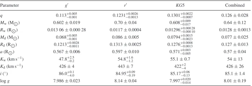
Table 3. System parameters for ASASSN-14ag from average light-curve fitting. The parameters in the combined column are calculated from the weighted mean of the values in each of the three bands. The errors on these combined parameters come from the weighted standard deviation of the parameters from the eight individual eclipse fits.

Parameter g r KG5 Combined

q 0.113+₋0₀._.005₀₀₁ 0.1231₋+0_0..0026₀₀₁₃ 0.1301₋+₀0._.0022₀₀₀₇ 0.126±0.028

Mw(M) 0.602±0.019 0.70±0.04 0.608+₋00..009017 0.64±0.12

Rw(R) 0.013 06±0.000 28 0.0117±0.0004 0.01296+₋00..000 28000 10 0.0128±0.0013

Md(M) 0.068+₋00..005001 0.086±0.005 0.0794+

0.0015

−0.0023 0.077±0.025

Rd(R) 0.1213+₋00..00280011 0.1313±0.0025 0.1276+

0.0008

−0.0013 0.127±0.013

a(R) 0.567±0.006 0.597±0.010 0.571₋+0₀._.003₀₀₅ 0.57±0.04

Kw(km s−1) 47.8₋+02..52 54.8+

1.6

−1.2 55.1±0.7 54±13

Kd(km s−1) 426±4 443±7 422+₋24 426±26

i(◦) 86.0₋+₄0._.1₀ 84.95+₋0_0..09₁₉ 85.17+₋0₀._.06₁₃ 85.1±1.4

logg 7.986±0.023 8.14±0.04 7.997₋+₀0._.020₀₁₄ 8.01±0.19

a white dwarf below 0.7 M and approaching the mean white dwarf field mass of 0.621 M (Tremblay et al.2016). The cor-responding donor mass of 0.093+₋00..015012M is consistent with the main-sequence donor evolutionary track from Knigge, Baraffe & Patterson (2011). These component masses give ASASSN-14ag an ∼95 per cent chance of lying within the dynamically stable region in fig. 2 of Schreiber, Zorotovic & Wijnen (2016), in agreement with their empirical consequential angular momentum loss model that appears to solve multiple issues with CV evolution.

The white dwarf temperature and mass were used to calculate a medium-term average mass transfer rate of

˙

M = 1.9+₋21..61 × 10−10 M yr−1 (Townsley & Bildsten 2003; Townsley & G¨ansicke2009), while ASASSN-14ag’s orbital pe-riod of 1.44 h was used to determine a secular mass transfer rate of

˙

M∼0.6×10−10_M

yr−1_{(Knigge et al.2011). While these two} values for the mass transfer rate are consistent, the slightly higher medium-term mass transfer rate indicates that the white dwarf tem-perature of 14 000+₋22002000 K is marginally hotter than we would expect.

6 C O N C L U S I O N S

We have introduced a new approach to modelling CV eclipses that enables multiple eclipses to be fitted simultaneously, with the option to model any inherent flickering with GPs. This no longer requires eclipses to be averaged together in order to overcome the presence of flickering, a technique employed in previous studies and subject to issues caused by disc radius changes.

This new approach has been tested using eight eclipses of the eclipsing CV ASASSN-14ag. These eclipses – all including flick-ering – were fitted simultaneously with and without GPs. Although both fits return a similar solution, the errors associated with the GP fit are much more representative given the large amount of flickering present.

We have shown GPs to be an effective way of modelling flickering and plan to use this new eclipse modelling approach on many more eclipsing CV systems going forward.

AC K N OW L E D G E M E N T S

We thank the anonymous referee for the useful comments. MJM ac-knowledges the support of a UK Science and Technology Facilities Council (STFC) funded PhD. SPL and VSD are supported by STFC grant ST/J001589/1. EB and TRM are supported by the STFC in

the form of a Consolidated Grant. VSD and TRM acknowledge the support of the Leverhulme Trust for the operation of ULTRASPEC at the Thai National Telescope. The results presented in this paper are based on observations made at the Thai National Observatory, operated by the National Astronomical Research Institute of Thai-land. This research has made use of NASA’s Astrophysics Data System Bibliographic Services.

R E F E R E N C E S

Ambikasaran S., Foreman-Mackey D., Greengard L., Hogg D. W., O’Neil

M., 2014, preprint (arXiv:e-prints)

Baptista R., Bortoletto A., 2004, AJ, 128, 411

Bell C. P. M., Naylor T., Mayne N. J., Jeffries R. D., Littlefair S. P., 2012, MNRAS, 424, 3178

Bergeron P., Wesemael F., Beauchamp A., 1995, PASP, 107, 1047 Bishop C. M., 2006, Pattern Recognition and Machine Learning.

Springer-Verlag, New York Bruch A., 2000, A&A, 359, 998 Bruch A., 2015, A&A, 579, A50

Dhillon V. S. et al., 2014, MNRAS, 444, 4009 Drake A. J. et al., 2009, ApJ, 696, 870

Earl D. J., Deem M. W., 2005, Phys. Chem. Chem. Phys., 7, 3910 Evans T. M., Aigrain S., Gibson N., Barstow J. K., Amundsen D. S., Tremblin

P., Mourier P., 2015, MNRAS, 451, 680

Feline W. J., Dhillon V. S., Marsh T. R., Stevenson M. J., Watson C. A., Brinkworth C. S., 2004, MNRAS, 347, 1173

Foreman-Mackey D., Hogg D. W., Lang D., Goodman J., 2013, PASP, 125, 306

Garnett R., Osborne M., Reece S., Rogers A., Roberts S., 2010, Comput. J., 53, 1430

Gelman A., Rubin D. B., 1992, Stat. Sci., 7, 457

Gianninas A., Strickland B. D., Kilic M., Bergeron P., 2013, ApJ, 766, 3 Gibson N. P., Aigrain S., Roberts S., Evans T. M., Osborne M., Pont F.,

2012, MNRAS, 419, 2683

Goodman J., Weare J., 2010, Commun. Appl. Math. Comput. Sci., 5, 65 Hellier C., 2001, Cataclysmic Variable Stars: How and Why they Vary.

Springer-Praxis, New York

Horne K., Wood J. H., Stiening R. F., 1991, ApJ, 378, 271 Kato T. et al., 2015, PASJ, 67, 105

Knigge C., Baraffe I., Patterson J., 2011, ApJS, 194, 28

Littlefair S. P., Dhillon V. S., Marsh T. R., G¨ansicke B. T., Southworth J., Baraffe I., Watson C. A., Copperwheat C., 2008, MNRAS, 388, 1582 Littlefair S. P., Dhillon V. S., G¨ansicke B. T., Bours M. C. P., Copperwheat

C. M., Marsh T. R., 2014, MNRAS, 443, 718 McAllister M. J. et al., 2015, MNRAS, 451, 114

at University of Warwick on January 9, 2017

http://mnras.oxfordjournals.org/

Rajpaul V., Aigrain S., Osborne M. A., Reece S., Roberts S., 2015, MNRAS, 452, 2269

Rasmussen C. E., Williams C. K. I., 2006, Gaussian Processes for Machine Learning. MIT Press, Cambridge, MA

Roberts S., Osborne M., Ebden M., Reece S., Gibson N., Aigrain S., 2013, Phil. Trans. R. Soc. A, 371, 20110550

Savoury C. D. J. et al., 2011, MNRAS, 415, 2025 Scaringi S., 2014, MNRAS, 438, 1233

Scaringi S., K¨ording E., Uttley P., Knigge C., Groot P. J., Still M., 2012, MNRAS, 421, 2854

Schlafly E. F., Finkbeiner D. P., 2011, ApJ, 737, 103

Schreiber M. R., Zorotovic M., Wijnen T. P. G., 2016, MNRAS, 455, L16 Shappee B. J. et al., 2014, ApJ, 788, 48

Smith J. A. et al., 2002, AJ, 123, 2121

Spark M. K., O’Donoghue D., 2015, MNRAS, 449, 175 Townsley D. M., Bildsten L., 2003, ApJ, 596, L227 Townsley D. M., G¨ansicke B. T., 2009, ApJ, 693, 1007

Tremblay P.-E., Cummings J., Kalirai J. S., G¨ansicke B. T., Gentile-Fusillo N., Raddi R., 2016, MNRAS, 461, 2100

Way M. J., Srivastava A. N., 2006, ApJ, 647, 102

Way M. J., Foster L. V., Gazis P. R., Srivastava A. N., 2009, ApJ, 706, 623 Wood M. A., 1995, in Koester D., Werner K., eds, Lecture Notes in Physics,

Vol. 443, White Dwarfs. Springer-Verlag, Berlin, p. 41

Wood J., Horne K., Berriman G., Wade R., O’Donoghue D., Warner B., 1986, MNRAS, 219, 629

This paper has been typeset from a TEX/LA_{TEX file prepared by the author.}

at University of Warwick on January 9, 2017

http://mnras.oxfordjournals.org/