Development of Fragility Curves for Multi Storey RC Structures

(1)

Development of fragility curves for multi-storey RC structures

Mr. Kolekar Shubham Sarjerao

1

_{, Dr. Patil Pandurang Shankar.}

2

1 _{M. Tech. student, Dept. of Civil-Structural Engineering, Rajarambapu Institute of Technology}₍_{An Autonomous}

Institute, Affiliated to Shivaji University), Islampur, Maharashtra, India

2_{Professor, Dept. of Civil-Structural Engineering¸ Rajarambapu Institute of Technology (An Autonomous Institute,}

Affiliated to Shivaji University), Islampur, Maharashtra, India

---*---Abstract -**

The damages to the structure which occur during an earthquake demonstrates the need for seismic evaluation of structure, which may predict the expected damages that may occur in the structure. This paper describes regarding vulnerability assessment of Multi-storey RC structures using fragility curves. Fragility curves helps to identify the probability of damages for a given damage states. Three different building models viz. G+1, G+3, G+12 storey have been considered and the fragility curves are generated for different damage states viz. slight, moderate, severe and complete. The building models are modelled as per the guidelines given by IS codes. The fragility curves are generated by using the guidelines given by HAZUS technical manual. Modelling is carried out using Sap2000 v19.

Key Words: Seismic action, Performance based analysis, Push over analysis, Sap 2000, HAZUS manual, fragility curves.

1. INTRODUCTION

The structures look strong from outside but may collapse immediately during an earthquake. Hence the structural components of any structure play a major role during earthquake. The structural components act as resisting elements and helps to prevent major damages that may occur during an earthquake. After the occurrence of Bhuj (Gujarat) earthquake in 2001, it was observed that most of the structures collapsed and lot of the damage occurred. There were numerous reasons for this damage, one such was the irregular use of the IS codes. Generally the structures cannot be made earthquake proof, it can be made earthquake resistant. Hence to make earthquake resistant structures performance based analysis can be carried out. The aim of performance based analysis is to predict the seismic action prior to the construction of structures and work accordingly. During analysis some uncertainties occur, which must be considered. Uncertainties involves estimation of performance of structure and seismic hazards. These uncertainties

mainly involves uncertainty of capacity, uncertainty of demand and uncertainty in modelling. In addition to uncertainties in the structure, seismic performance and seismic vulnerability of the structure for given seismic parameters should also be considered. Seismic vulnerability of structure is generally expressed in terms of probabilistic function which represents the damage states for the particular structure. The damage states are represented in terms of curves known as fragility curves. To trace fragility curves, analytical approach is adopted.

2. PUSH OVER ANALYSIS

Push over analysis is used to trace fragility curves. Push over analysis is a non-linear static analysis method, where the structure is first subjected to gravity loading which comprises of dead and live load pattern subjected to a full load condition of elastic and inelastic behavior till ultimate condition is reached. While analyzing a frame or a structure all kinds of non-linearity as mentioned previously are considered, by assigning the hinges at proper location where the plastic rotation is governed as per FEMA-356. Non-linear parameters like P-Delta effect, link assignments and staggered construction are considered by software itself while doing analysis.

After the final analysis the static pushover curves are obtained which are the plot of strength based parameters against deflection. These curves are further used for different study purposes.

After analysis the results for ductile capacity of frame or structure, load level and deflection at failure point is obtained.

The curves obtained after push over analysis are as shown below,

2.1. Capacity curve

(2)

typical capacity curve is as shown in fig. 1

Fig. 1 Capacity curve

2.2. Capacity spectrum

To convert capacity curve into capacity spectrum, equation given in ATC-40, volume- 1, p-8.9 can be used. A typical capacity spectrum curve is as shown in fig. 2

Fig. 2 Capacity spectrum

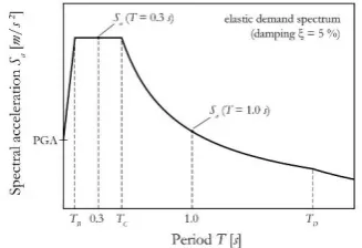
2.3. Demand curve

This curve represents earthquake ground motion. This curve is a plot of spectral acceleration (Sa) vs time period (T). A typical demand curve is as shown in fig. 3

Fig. 3 Demand curve

2.4. Stages of plastic hinges

Fig. 4 Stages of plastic hinge

The graph is a plot of base shear and displacement. The plot is obtained after pushover analysis. The notation IO, LS, CP represents immediate occupancy, life safety and collapse prevention. From the plot the region AB represents elastic range, B to IO is the range for immediate occupancy, IO to LS is the range for life safety, LS to CP is the range for collapse prevention. As the curve reaches at point C, maximum deformation is reached and curve drops down linearly and the stage of failure is reached. After this point the force remains constant up to certain limit.

3. HAZUS METHODOLOGY

Various methods can be used for the evaluations of fragility curves. However, HAZUS manual can also be used for tracing of fragility curves. It was first used by National Institute of Building Science (NIBS) to reduce the hazards in United States. In this manual procedure for tracing of fragility curves for different types of structure is given. Fragility curves is a tool of determining the probability of structural and non-structural damages in the structure. Fragility curves are derived by using a log normal function.

The log-normal function can be given as follows,

P (ds/sd) = ɸ [

Where,

sd,ds = Threshold spectral displacement for a given damage state.

βds = Standard deviation of natural logarithm of the

damage state.

ɸ = Standard normal cumulative distribution function.

sd = Spectral displacement of the structure. P [S | sd] = probability of being in or exceeding a slight damage state, S.

[image:2.595.362.505.110.216.2] [image:2.595.84.238.128.264.2] [image:2.595.91.231.339.457.2] [image:2.595.77.241.547.659.2]

(3)

extensive damage state, E.

P [C | sd] = probability of being in or exceeding a complete damage state, C.

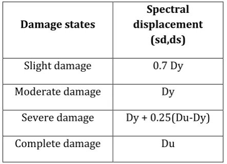
[image:3.595.51.273.218.378.2]

Damage states at a particular spectral displacements can be evaluated by using following table,

Table 1. Spectral displacement and damage states

Damage states

Spectral displacement

(sd,ds)

Slight damage 0.7 Dy

Moderate damage Dy

Severe damage Dy + 0.25(Du-Dy)

Complete damage Du

4. PROCEDURE FOLLOWED FOR MODELLING IN SAP2000

1.) Basic model is created using desired dimensions. 2.) Define material properties viz. grade of concrete and grade of steel. Grade of steel is assigned by using rebar properties.

3.) Define the frame section properties, viz. size of beam, size of column, etc… and also assign the slab thickness using area section properties.

4.) Assign all the frame and area sections at desired locations properly.

5.) Load patterns are defined which includes dead loads, live loads and seismic loads. Care should be taken that while assigning a live load, load is assigned by reductions give in codes. A single seismic load can be defined for symmetric structure but in practice we come across unsymmetrical structures, so separate load pattern for x and y direction should be defined. 6.) After assigning load patterns properly, load cases are defined. Along with load cases for dead, live and seismic additional load cases are to be included. Gravity load case is assigned after old load cases. Gravity load case is a non-linear case which includes only dead and live load. Assign mass-source and P-delta effect correctly. Generally this load case is considered for full load condition and all final

displacement values are considered. After gravity case push over case is assigned which is also a non-linear case. Here the multi-step displacements are considered.

7.) After assigning all the load cases, load combinations are given. One can choose the default load combinations or we can also give it manually.

8.) Hinge properties are assigned to both beams and columns for gravity case/combo and added at zero and one location.

9.) Run the model, analysis will be carried out and static pushover curves will be generated.

10.) To trace fragility curves select FEMA440 displacement curves and note values of Du and Dy from table 1 and table 2, available in table tab.

5. MODELLING AND ANALYSIS

To study push over analysis, three different models of different storey are considered viz. G+1, G+3 and G+ 12. Modelling and analysis is carried out using sap2000. The data commonly used for the 3 models are given below.

The general properties considered during modelling are as follows,

 Modulus of elasticity of steel, Es= 2 x 105_MPa  Modulus of elasticity of concrete, Ec= 27386.12

MPa

 Grade of concrete= M25 Details of modelling

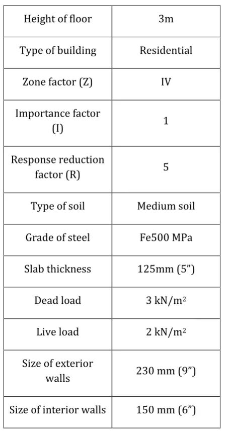
Seismic parameters considered for modelling are as per the standards of IS 1893 (Part 1) 2016 and are tabulated as below,

Table 2. Parameters considered for modelling

Type of building R.C.C.

Plan area 20m x 20m

Height of building

(Including height of plinth = 1m)

G+1- 7m

G+3- 13 m

(4)

Height of floor 3m

Type of building Residential

Zone factor (Z) IV

Importance factor

(I) 1

Response reduction

factor (R) 5

Type of soil Medium soil

Grade of steel Fe500 MPa

Slab thickness 125mm (5”)

Dead load 3 kN/m2

Live load 2 kN/m2

Size of exterior

walls 230 mm (9”)

Size of interior walls 150 mm (6”)

5.1. Loads considered in analysis

Following are the loads considered during the analysis of structure.

1.) Gravity loads:

Intensity of loads considered in the study, at different floor levels are tabulated as below,

[image:4.595.50.277.94.523.2]

a.) Dead load

Table 3. Dead load used in analysis

Weight of slab 0.125 x 25 3.00

kN/m2

Weight of floor

finish ( Including 3

3 kN/m2

other dead load)

Weight of partition wall

0.23 x 1 x 3 x 20 (For

exterior wall)

0.15 x 1 x3 x20 (For

interior wall)

13.8 kN/m

(For exterior

wall)

9 kN/m (For interior

wall)

b.) Live load

Live load for all the floors are considered as 2 kN/m. As per the codal provisions of IS 1893 it is reduced by 25% since the dead load considered is less than 3.5 kN/m2_.

2.) Seismic load:

Seismic load parameters are considered as per IS 1893 (Part 1) 2016. Software considers a lumped mass of system at each floor level. The dead and live loads considered over the beam, column and slab surfaces are distributed uniformly over the surface. The following parameters are considered during analysis, a.) Zone factor (Z)

The structure is considered to be lying in zone IV and taken as 0.24.

b.) Response reduction factor (R)

The frame is considered as a special moment resisting frame (SMRF) and so response reduction factor is considered as 5 for the analysis.

c.) Damping ratio

According to the codal provision of IS 1893 (Part 1) 2016, for normal concrete structures the damping is considered as 5%.

d.) Soil type

Medium soil (Type 2) is considered during analysis.

6. RESULTS AND DISCUSSION

(5)

walls and other parameters required are considered as mentioned in table 2 and table 3. Spectral displacements are taken as ground motion parameter.

6.1. Building model 1 (Low-rise building)

The three dimensional model of G+1 RCC frame is considered. The size of beam and columns are 230mm x 230 mm and 300mm x 300mm respectively. All other parameters required are tabulated in table 2 and table 3.

Fragility curves developed after analysis for all damage states are shown in fig. 5

Fig. 5 Fragility curves for Building model 1

6.2. Building model 2 (Mid-rise building)

[image:5.595.320.547.133.282.2]

The three dimensional model of G+3 RCC frame is considered. The size of beam and columns are mentioned in table 4.

Table 4. Sizes of beams and column for building model 2

Particulars Sizes

Beams at plinth level 230mm x 230mm

Beams at floor level 230mm x 450mm

Column at footing and

1st_floor. 300mm x 450mm

Column at 2nd_{, 3}rd_and

4th_floor. 300mm x 300mm

All other parameters required are tabulated in table 2 and table 3.

Fragility curves developed after analysis for all damage states are shown in fig. 6

6.3. Building model 3 (High-rise building)

[image:5.595.36.260.293.434.2]

The three dimensional model of G+12 RCC frame is considered. The size of beam and columns are mentioned in table 5.

Table 5. Sizes of beams and column for building model 3

Particulars Sizes

Beams at plinth level 230mm x 450mm

Beams at floor level 230mm x 530mm

Column at footing, 1st

and 2nd floor. 300mm x 750mm

Column at 3rd, 4th_and

Column at 6th_{, 7}th_and

Column at 9th_{, 10}th_and

All other parameters required are tabulated in table 2 and table 3.

[image:5.595.324.544.415.659.2] [image:5.595.51.271.568.730.2]

(6)

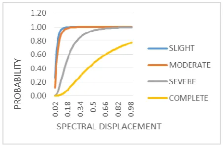
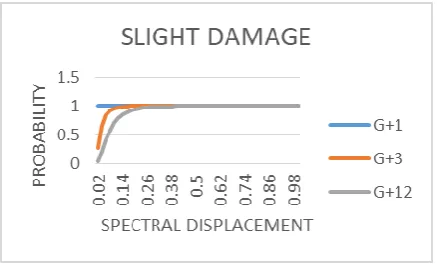
Combine graphs for all building models for individual damage states are shown below,

Fig. 8 Combined graph for slight damage state for all building models

Fig. 9 Combined graph for moderate damage state

[image:6.595.320.545.274.409.2]

for all building models

[image:6.595.36.255.296.428.2]

Fig. 10 Combined graph for severe damage state for all building models

Fig. 11 Combined graph for complete damage state

for all building model

SUMMARY AND CONCLUSION

In this paper, methodology for tracing of fragility curves have been discussed by using the guidelines of HAZUS manual. Fragility curves for low-rise, mid-rise and high-rise building models have been traced. From the results, it is clear that the HAZUS manual helps to give us values of damage state for particular spectral displacement.

From the results it is clear that all the building models undergoes slight and moderate damages, this can corrected by using minor retrofitting techniques. G+1 building model shows more damages, so the sectional properties of the structure should be either increased or retrofitting techniques like jacketing for columns and other structural components should be done.

ACKNOWLEDGEMENT

[image:6.595.47.276.465.602.2]

(7)

REFERENCES

[1

] Dakshes J. Pambhar (2012), “Performance based Pushover Analyis of R.C.C. Frames”-IJAERS- International Journal of Advanced Engineering Research and Studies

, volume I

[2] HAZUS MR4 technical manual developed by Department of Homeland security, Emergency Preparedness and Response Directorate, FEMA Mitigation Division, Washington, D.C.

[3] Kiran Kamath and Anil S (2017), “Fragility curves for low-rise, Mid-rise and high-rise concrete Moment resisting frame building for

Seismic vulnerability assessment”-IJCIET- International Journal of Civil Engineering and Technology, volume 8. [4] Karthik J and Dr. B. Shivakumara Swamy (2018), “Fragility Analysis of RC Framed Structure For Different Seismic zones”-IRJET-International Research Journal of Civil Engineering and Technology, volume 5. [5] Megha Vasavada and Dr. Dakshes J. Pambhar (2012), “Performance based Pushover Analyis of R.C.C. Frames”-IJAERS- International Journal of Advanced Engineering Research and Studies, volume I.

[6] Vazurkar U. Y. and Chaudhari, D. J. (2016), “Development of Fragility Curves for RC Buildings”-IJER, International Journal of Engineering and Research, volume 5.

BIOGRAPHIES

Mr. Kolekar Shubham Sarjerao, M.Tech. Structural Engineering student,

Department of Civil Engineering, Rajarambapu Institute of Technology (An Autonomous Institute, Affiliated to Shivaji University), Islampur, Maharashtra (India)-415414

Dr. Patil Pandurang Shankar, Professor,

Development of Fragility Curves for Multi Storey RC Structures