Efficient analysis of data streams

(1)

Efficient Analysis of

Data Streams

Rhian Natalie Davies

Submitted for the degree of Doctor of Philosophy

at Lancaster University.

(2)

Abstract

Data streams provide a challenging environment for statistical analysis. Data points can arrive at a high velocity and may need to be deleted once they have been observed. Due to these restrictions, standard techniques may not be applicable to the data streaming scenario. This leads to the need for data summaries to represent the data stream. This thesis explores how data summaries can be used to perform clustering and classification on data streams across a broad range of applications.

Spectral clustering is one such technique which prior to this work has not been applicable to the data streaming setting due to the high computation involved. CluStream is an existing method which uses micro-clusters to summarise data streams. We present two algorithms which utilise these micro-cluster summaries to enable spectral clustering to be performed on data streams. The methods were tested on simulated data streams, as well as textured images and hand-written digits.

(3)

high-dimensional clustering problem and uses the cluster labels to identify changes within the signal.

(4)

Acknowledgements

I would like to thank my supervisors Dr Nicos Pavlidis and Professor Idris Eckley for their endless support, guidance and patience throughout this project. This final version of the thesis has been improved thanks to the helpful comments of my viva examiners, Dr Sotirios Tasoulis and Professor Kevin Glazebrook. Thanks are also due to Professor Lyudmila Mi-haylova for her help with the conference paper presented in Chapter 4. The data analysed in Chapter 3 was kindly provided by Shell.

My PhD has been supported by the EPSRC funded Statistics and Operational Research (STOR-i) Centre for Doctoral Training. The STOR-i CDT has provided an excellent research environment and many additional training opportunities which have allowed me to develop my research skills. Particular thanks go to the STOR-i director Professor Jonathan Tawn for his constant support, especially during the late PhD stages.

I would also like to give special thanks to the ‘11-‘15 cohort of STOR-i: Ben, Dave, Emma, Hugo, James, Judd, Rob and Tom. My PhD experience was greatly enhanced by their knowledge, encouragement and friendship.

(5)

Declaration

I declare that the work in this thesis has been done by myself and has not been submitted elsewhere for the award of any other degree.

I declare that the word count of this thesis is 23469 words.

Chapter 4 has been accepted for publication as R. Davies, L. Mihaylova, N. Pavlidis, and I. A. Eckley. The effect of recovery algorithms on compressive sensing background subtraction.

In Sensor Data Fusion: Trends, Solutions, Applications, 1 - 6, 2013.

(6)

Chapter 1 Introduction

The volume of data collected on a daily basis is staggering. In 2013, IBM stated that over 90% of the world’s data was created in the last two years. This creates a challenge for researchers and practitioners as computers may not have the memory requirements to deal with such large quantities of data, and their algorithms may not run fast enough or even at all. Big data (Buhlmann et al., 2016) is a term used to refer to data sets so huge that traditional statistical techniques may not be directly applicable.

(10)

collection (Shankar et al., 2016); oil and gas including the development of the digital oil field which uses sensors throughout oil wells to monitor flow and other operational characteristics (Cramer et al., 2008; Patri et al., 2012).

The rate at which data arrives could be as fast as millions of data points each hour such as in the Macy’s and oil company examples. However, even if the data arrives more slowly, this can still provide a challenge if the available processing power, storage capabilities or transmission rates are limited.

It is possible for a data stream to be unbounded in size by which we mean that there is no time point where the data stream ends. This is common in data streams found in meteorology, the stock market, online shopping and social media. Since these data streams are potentially endless in size it is not possible to store the data in its entirety. This means that instead of performing analysis once the data has been collected, analysis must be performed and updated in real time as new data points are observed. This leads to another issue sometimes referred to as the one-pass-access problem. As data streams are processed serially, once a data point has been seen it is discarded and cannot be accessed again. Some seemingly trivial analyses such as computing the median of the data become impossible in the data stream setting because of this one-pass-access issue. In fact, many statistical techniques make assumptions which do not hold in the data streaming scenario. A summary of the restrictions imposed by data streams is given below (Silva et al., 2013):

1. Data objects arrive continuously.

2. There is no control over the order in which the data objects should be processed.

(11)

4. Data objects are discarded after they have been processed.

5. The unknown data generation process is possibly non-stationary.

Given the restrictions above, how can we perform analysis on a data stream? If the issue was just the size of the data then we could sample and perform analysis on that sample. However as the data stream cannot be stored, it is not possible to take a sample of the whole stream. We could sub sample as we go along based on the frequency storing every 100th data point. However, if the data stream is unbounded then eventually this method will fail. What is needed is a representative data summary of the data stream that captures the new data points but still retains some historical information. An ideal representative data summary will:

1. Be computationally easy to update.

2. Store historical information.

3. Forget historical information if it becomes obsolete.

4. Adapt if the underlying generating process of the data stream changes.

5. Be informative enough to use in statistical analysis.

(12)

window will retain historical information but may be slow to update to a change in the data stream. This will naturally infer a temporal bias and a poorly selected window size may lead to missing important seasonal trends such as the effect of Christmas on shopping sales.

We discussed above how it is not possible to calculate the median of a data stream. It is however quite simple to keep a track of the running mean by storing the sum of the data points and the number of data points observed so far. This is another simple example of a representative data summary. Again it is computationally easy to update and all historical information can be retained. However, in order to perform clustering or regression on the data stream we will need a richer data summary than just a running mean.

Once a suitable representative data summary has been selected, this can then be used to perform analysis such as clustering. However standard techniques might need to be adapted to work on these data summaries as opposed to on the raw data. In this thesis we explore the use of representative data summaries on the analysis of data streams.

1.1 Thesis Outline

In Chapter 2 we consider the problem of identifying groups or clusters in a data stream. Many different types of clustering algorithms exist however, we restrict our interests to spectral

clustering. Spectral clustering is popular, offers good empirical performance and can handle

tricky, non-Gaussian data sets. However, due to it’s complexity it cannot be performed on very large data sets and is not suitable for data streams.

(13)

algo-rithm spectral CluStream, which summarises data streams and performs spectral clustering on those data summaries. A spectral clustering algorithm which can cluster data streams does not currently exist in the literature. We consider both weighted and un-weighted vari-ants of online spectral clustering. A number of different data sets are analysed including handwritten digit data and wavelet based texture features from an image data set.

Chapter 3 uses CluStream to identify corruption within acoustic sensing signals. Dis-tributed acoustic sensing (DAS) is a modern technique used to monitor oil flow at various depths throughout an oil well. DAS uses a fibre-optic cable to record vibrations at very high resolutions, up to 10000 observations a second. DAS is fairly cheap to implement and offers high frequency data, but unfortunately corruption can occur in the signal. Our challenge is to identify the locations in the signal where corruption occurs. Existing methods for detecting and removing interference in DAS signals involve using offline, uni-variate changepoint de-tection. However DAS signals are multivariate and require online processing. We show that CluStream provides an alternative approach to changepoints analysis to identify corruption within DAS signals.

(14)

recovery algorithms on CCTV surveillance footage.

All three chapters are linked by the challenge of gaining insight from data streams by analysing a simple summary of the stream and extrapolating the analysis to learn something about the data stream as a whole. Contributions of this thesis and observations on data stream analysis are gathered in Chapter 5 with suggestions for future areas of research.

In summary, the main contributions of this thesis are:

• A new method, Spectral CluStream that enables Spectral clustering to be performed in

the data streaming environment.

• A study of the weighting micro-clusters in Spectral CluStream.

• A novel application of online clustering to segment Distributed Acoustic Sensing data.

• An empirical comparison of two competing recovery algorithms in the compressive

(15)

Chapter 2 Spectral Clustering for Data Streams

2.1 Introduction

The goal of clustering algorithms is to separate data into groups or clusters such that data points within a cluster are similar, and data points in different clusters are dissimilar (Everit et al., 2001). Many different types of clustering algorithms exist including centroid type methods such as k-means (MacQueen, 1967; Lloyd, 1982) and density based algorithms like DB-Scan (Ester et al., 1996). In this chapter, we consider the challenge of data stream clustering. Adata stream (Gama, 2010; Silva et al., 2013) is data which arrives in an ordered sequence. It is potentially unbounded in length and arrives continuously. Examples can be found in many applications such as telecommunications, shopping transactions and customer click data. For example, an insurance company will receive millions of quote requests an hour, and by clustering these quotes they may be able to better understand their customer base and adapt their services to meet requirements.

(16)

Schweitzer, 2013; Song et al., 2013), which are able to effectively handle a large volume data stream. However, the performance of these streaming clustering algorithms tends to diminish when the underlying nature of the data stream is non-Gaussian. For example, the clusters generated from a streaming k-means algorithm are always convex sets. There is the need for a clustering algorithm which can handle data streams with less restrictive assumptions on the form of the clusters. To overcome this problem, we propose a streaming adaptation of the spectral clustering algorithm. Spectral clustering (von Luxburg et al., 2008) is a clustering method which uses the eigenvalues of an affinity matrix of the data to perform dimension reduction and cluster in the lower dimensional space. Spectral clustering is popular, offers good empirical performance and crucially, can the handle tricky, non-Gaussian data which other streaming clustering algorithms struggle to cluster. An introduction to spectral clustering is given in Section 2.2.

There does not exist an algorithm for performing spectral clustering on data streams, however, advanced spectral clustering techniques exist, which are discussed in Section 2.3. These algorithms address some of the issues met in data streaming, by working with large scale data or incremental data sets but do not meet all the challenges of implementing spectral clustering in data streams. In particular, these algorithms cannot deal with the fact that data streams can be potentially unbounded in size. The need for a spectral clustering algorithm which can truly be applied to data streaming is apparent.

(17)

their performance on simulated and real data in Section 2.5. Conclusions and future work are discussed in Section 2.6.

2.2 Spectral Clustering Background

In this section we motivate spectral clustering and introduce the spectral clustering algorithm by first noting the link between spectral clustering and graph partitioning problems.

As discussed in Section 2.1 the goal of clustering algorithms is to partition data X =

{x1, . . . , xn}, xi ∈Rd, intok disjoint clusters such that eachxi belongs to exactly one cluster.

Data sets can have underlying true clusters of all shapes and sizes, for example, they can be spherical and convex as in Figure 2.2.1a or connected but non-convex as in Figure 2.2.1b.

(a) Convex clusters. (b) Non-convex clusters.

Figure 2.2.1: Examples of different types of clustering problems. The clusters in Figure 2.2.1a are generated by a multivariate Gaussian distribution. The clusters in Figure 2.2.1b are non-convex which makes the clustering problem more difficult.

(18)

given in Figure 2.2.1a. However k-means can fail when the true clusters are non-convex like those shown in Figure 2.2.1b. This is because k-means is a centroid based clustering algorithm that clusters data based on how similar they are to cluster centroids. Spectral clustering instead clusters data based on how similar they are to all other data points, which can lead to good quality segmentation on even these difficult cases. We do not formally address what is meant by similarity here, but will define this fully in Section 2.2.2.

The similarity between data points can be neatly represented in a graph structure. We can then restate the clustering problem as a graph partitioning problem where we wish to find a partition of the graph such that the edges between different groups have low weights (which corresponds to data points being dissimilar) and the edges within a group have high weights (the data points are similar). In order to introduce spectral clustering we first introduce some graph notation and discuss graph cut problems. We will then describe the spectral clustering algorithm, and discuss in more detail the notion of similarity.

2.2.1 Graph cut problems

Data can be represented as a similarity graph,G= (V, E) where each vertexvi ∈V represents a data pointxi. The graph will be undirected, by which we mean the edges denote a two-way

relationship. The graph can then be described by an adjacency matrix. Adjacency matrices are a way of depicting the graph structure with binary entries denoting which vertices are connected by edges and which are not. Figure 2.2.2 depicts two similarity graphs and their corresponding adjacency matrices. A value of 1 in cell (2,3) implies that vertices v2 and v3

(19)



  

0 1 0 1 1 0 1 0 0 1 0 1 1 0 1 0



  



  

0 1 1 1 1 0 0 0 1 0 0 0 1 0 0 0



[image:19.612.157.456.76.258.2]

  

Figure 2.2.2: Two example similarity graphs and their corresponding adjacency matrices.

The weighted adjacency matrix (also called an affinity matrix) of a similarity graph is

the matrix W = (wij)i,j=1,...,n. The weight wij is the similarity between vertices vi and vj.

If wij = 0, this means that the vertices vi and vj are not connected by an edge. Again the

affinity matrix will be symmetric, that is wij =wji.

In order to create a graph partition we need to cut the edges in the graph. Non-empty subsets of V, A and B will form a partition of the graph G if A∩B = ∅ and A∪B = V. The weight of the cut can be calculated by summing the weights of the edges which will be broken when a cut is made. In order to find a good partition of the graph, we wish to choose

A and B such that some cut criterion is minimised. The simplest cut criterion is

cut(A,B) = X

i∈A,j∈B

wij, (2.2.1)

where the notation i∈A is short hand to mean the set of indices {i|vi ∈A}.

(20)

not always produce a desirable graph partitioning; it tends to create unbalanced partitions, separating one vertex from the rest of the graph. To understand why this happens, note for a fully connected graph where all vertices are joined by an edge, the number of edges cut in mincut will be |A| × |B| which is minimised by the solutions |A| = 1 or |B| = 1. In order to avoid this, we can specify that the sets A and B are reasonably large in some way. Two common objective functions used to avoid this issue are the RatioCut (Hagen and Kahng, 1992) and the normalised cut, Ncut (Shi and Malik, 2000).

Both RatioCut and Ncut attempt to normalise the weight of the cut by introducing the size of sets A and B. In RatioCut, the size of A is measured by its number of vertices

|A|, while in Ncut the size is measured by the weights of its edges vol(A) = P

i∈Adi where

di =

Pn

j=1wij is the degree of a vertex vi ∈V. The definitions of RatioCut and Ncut are as

follows,

RatioCut(A,B) = cut(A, B)

|A| +

cut(A, B)

|B| , (2.2.2)

Ncut(A,B) = cut(A, B) vol(A) +

cut(A, B)

vol(B) . (2.2.3)

(21)

(a) Minimising the cut. (b) Minimising the normalised cut.

Figure 2.2.3: Two solutions to the bi-partition problem. The partitioning is indicated by shading/non-shading of nodes.

Although the partitioning has been improved, the previously easy to solve mincut problem (equation 2.2.1) has been replaced with minimising the normalised cut (equation 2.2.3) which is an NP-hard problem (Wagner and Wagner, 1993). Therefore, a continuous relaxation of the Ncut is solved instead. The solution to the relaxed problem of equation (2.2.3) is given by the second eigenvector of the symmetric graph Laplacian defined in equation (2.2.5) (von Luxburg et al., 2008). Similarly, the solution of the relaxed problem the ratio cut (equation 2.2.2) is given by the second eigenvector of the unnormalized Laplacian defined in equation (2.2.4). Here W is the affinity matrix of the similarity graph and the degree matrix D is defined as the diagonal matrix with the degrees d1, . . . dn on the diagonal. The relaxation of

these graph cut problems into the eigen-decompostion of Laplacian matrices is the basis of spectral clustering.

L= D−W. (2.2.4)

(22)

Unfortunately, there is no guarantee on the quality of the solutions of the relaxed problems compared to the exact solutions (Chung, 1997). Consequently, it has been shown that some pathological cases exist which are arbitrarily bad. However, several papers which investigate the quality of the clustering of spectral clustering (Spielman and Teng, 1996; Kannan et al., 2004) find spectral clustering to provide good solutions.

The spectral clustering algorithm that we use (Ng et al., 2001) uses the symmetric Lapla-cian Lsymm as defined in equation 2.2.5. The full spectral clustering algorithm is given in

Algorithm 1. Note that the number of clusters is assumed to be known and this will be the case throughout this chapter.

Algorithm 1 NJW spectral clustering algorithm

Input: Data set X ={x1, . . . , xn}, number of clusters k.

Output: k-way partition of the input data.

1: Construct the affinity matrix W = (wij)i,j=1,...,n.

2: Compute the symmetric Laplacian matrix Lsymm=D−1/2(D−W)D−1/2, where Dis the

diagonal matrix with Dii=

Pn

j=1wij.

3: Compute thek eigenvectors ofLsymm, v1, v2, . . . , vk,associated with thek smallest eigen-values, and form the matrix V = [v1, v2, . . . , vk].

4: Renormalise each row of V to form a new matrix Y. 5: Partition the n rows ofY into k clusters using k-means.

6: Assign the original data point xi to the clusterl if and only if the corresponding rowi of

the matrix Y is assigned to the cluster l.

(23)

each column is an eigenvector of the Laplacian, with length n. We can view this matrix Y as an embedding of the original data X into a lower dimensional subspace. When represented in this low subspace the clustering problem is often easier, and can be solved with a simple clustering algorithm such as k-means. For example, Figure 2.2.4a shows a data set of three spirals depicted in the original feature space. This is visually quite difficult to cluster. Figure 2.2.4b plots the same data set but embedded in the lower dimension, plotting the first eigen-vector of the Laplacian against the second eigeneigen-vector. Clustering in the embedded space is easy even for k-means to solve.

(a) Data viewed in the original feature space.

(b) Data viewed in the 2-dimensional embedding space.

Figure 2.2.4: Triple spiral data set viewed in feature space (a) and eigenvector space (b).

After the embedding, k-means can be used to cluster the n rows of Y into k clusters. Finally, assign the cluster label given to each rowYi to the corresponding original data point xi. Now that we have introduced the general spectral clustering algorithm, we will discuss

(24)

2.2.2 Choice of affinity matrix

One of the key factors of spectral clustering is the affinity matrix W = (wij)i,j=1,...,n which

represents the pairwise similarities between all data points xi and xj. A popular choice is to

use the Gaussian kernel,

wi,j = exp

−kxi−xjk

2

2σ2

, i, j = 1, . . . , n, (2.2.6)

where the parameter σ controls the width of the local neighbourhoods which we want to model. Ifxiandxj are very close, thenwij →1, and if they are far apartwij →0. A Gaussian

kernel affinity matrix will have ones along the diagonal and is symmetric (wij =wji).

The scaling parameter σ is usually chosen manually. Ng et al. (2001) automatically choose σ by running their clustering algorithm repeatedly for a number of values ofσ. They then select the σ which provides least distorted k-means clusters in step 5 of Algorithm 1. Zelnik-manor and Perona (2004) argue that for data which has a cluttered background, or multi-scale data, one global parameter choice forσis not sufficient. They calculate a localised parameter σi for each data point xi based on its neighbourhood. Using a localised σi can

deal well with multi-scale data, but requires the user to choose the size of the neighbourhood in order to calculate σi.

If we mainly wish to model the local relationships then using all of the possible pairwise data similarities may not be necessary. It is possible to use a weighted k-nearest neighbour structure (von Luxburg et al., 2008) to build the affinity matrix once corrections have been made to ensure that this matrix is symmetric. Another option is to choose some threshold

(25)

than this threshold . This is an -neighbourhood graph as shown in equation (2.2.7).

w_ij∗ =

   

  

1, if wij >

0, otherwise.

(2.2.7)

Using this construction will give a sparse affinity matrix instead of a fully connected graph, which will help lower the computational complexity.

2.3 Advanced Spectral Clustering

In the previous section we introduced spectral clustering via graph partitioning and discussed options for creating affinity matrices. Our overall aim is to perform spectral clustering on data streams. First, we consider some of the challenges that make clustering in data streams so difficult, and look at the approaches that exist to deal with these challenges in the spectral clustering setting.

The first challenge that is addressed is dealing with big data. One of the main difficulties in data streaming is the pure volume of data available and the methods discussed in Section 2.3.1 offer methods to perform spectral clustering on big data. Another difficulty that arises in data streaming is the ability to update the current clustering result as new data arrives. Incremental spectral clustering is a potential solution to this challenge and is discussed in Section 2.3.2.

(26)

clustering result if a new data point arrives. The incremental spectral clustering algorithms can update cluster membership as new data arrives but do not scale as for very large or possibly infinite n.

2.3.1 Large-scale Spectral Clustering

Spectral clustering can be challenging for very large data sets since constructing the affinity matrix W and computing the eigenvectors of L have computational complexity O(n2) and

O(n3_{) respectively. The Nystr¨}_{om method (Williams and Seeger, 2001) is a general method}

for generating good quality low rank approximations of large matrices. The Nystr¨om approx-imation method for spectral clustering (Fowlkes et al., 2004) randomly samples the columns of the affinity matrixW and approximates the eigen decomposition of the full matrix directly using correlations between the sampled columns and the remaining columns. Effectively this can be thought of as a dial which the user has control over, sampling more columns will provide better results but at a higher computational cost. The downsides with this method are that the memory requirements can be high and the random sampling of columns may lead to small clusters being under represented or completely missed in the final clustering.

(27)

the spectral clustering. In both Yan et al. (2009) and Shinnou and Sasaki (2008) the cluster labels given to the original data points are the same as the label assigned to their nearest representative point. As an alternative, Chen and Cai (2011) represents the data as a linear combination of representative points. Random sampling has been applied to reduce the size of the data points within the eigen-decomposition step. Chen et al. (2006); Liu et al. (2007) introduce early stopping strategies to speed up eigen-decomposition based on the observation that well-separated data points will converge more quickly to the final embedding. However this is only suitable for binary clustering. Other possibilities include random projection with sampling methods (Sakai and Imiya, 2009) and shortest path methods (Liu et al., 2013).

We discuss the KASP algorithm in more detail as it is the most popular speed up method for spectral clustering and it inspired our work in online spectral clustering which is intro-duced in Section 2.4.

In KASP, k-means is applied with q clusters to the data set X, where q is chosen such that k q n. Therefore each point in X belongs to a cluster yj,(j ∈ 1, . . . , q). Let

the centres of these q clusters be y1, . . . ,_b yq_b. These are used as representative points for the whole data set. Spectral clustering is performed on the representative points, reducing the complexity of the eigen decomposition fromO(n3_{) to} _O₍_q3_{). Finally, the original data points}

are assigned the cluster label that their closest representative point yj_b was assigned in the spectral clustering. The KASP algorithm is given in Algorithm 2.

Both KASP and RASP have been shown to perform well empirically on large data sets (Yan et al., 2009), retaining good clustering performance even as the data reduction ratio

(28)

Algorithm 2 KASP

Input: Data set X =x1, . . . , xn, number of clusters k, number of representative points q. Output: k-way partition of the input data.

1: Perform k-means with q clusters on x1, . . . , xn to create clustersy1, . . . yq.

2: Compute the cluster centroids y1_b, . . . ,yq_b as the q representative points.

3: Build a correspondence table to associate each xi with the nearest cluster centroids ybj.

4: Run a spectral clustering algorithm on y_b1, . . . ,ybq to obtain ank-way cluster membership

for each of yj_b,(j ∈1. . . q).

5: Recover the cluster membership for eachxi by looking up the cluster membership of the

corresponding centroid y_bj in the correspondence table.

(29)

The methods discussed above only address dealing with large data sets which are static. Our aim is to investigate methods which can update the spectral clustering partitioning when new data points arrive.

2.3.2 Incremental methods for Spectral Clustering

(30)

eigenvectors.

The first method is described in Valgren and Lilienthal (2008). When new points arrive, the spectral clustering is updated directly using a similarity threshold to assign points to clusters. If a new data point is sufficiently far from its closest representative points, it is considered the start of a new cluster. This means that the number of overall clusters must always increase. Therefore it is not feasible for data streams. In addition there is no method for splitting existing clusters as new data points arrive.

(31)

Kong et al. (2011) is a mixture of both Ning and Valgren’s methods, using representative points like Valgren but the eigen-updating of Ning. Although it can be quicker that Ning it retains the other issues of Ning’s method discussed above. In addition it has the same problem of Valgren’s method that the number of clusters increases over time. This makes it unsuitable for data streams.

Although the methods discussed deal with some aspects of difficulties in data streams, none of them are suitable for the full problem of clustering a data stream. We introduce an online spectral clustering algorithm for data streams based on the CluStream model of Aggarwal et al. (2003) in Section 2.4.

2.4 CluStream for Spectral Clustering

In this section, we first review a number of general methods for data stream clustering, although none of these offer spectral clustering for data streams. We then discuss the CluS-tream algorithm in more depth and introduce our algorithm, spectral CluSCluS-tream. Finally, we consider whether to weight micro-clusters within the spectral CluStream algorithm.

2.4.1 Data Stream Clustering

(32)

One of the first algorithms able to identify clusters in large and incremental data sets was BIRCH (Zhang et al., 1996). BIRCH achieved this by using cluster feature vectors to summarise the data stream and perform hierarchical clustering. BIRCH exploits the observation that the feature space is not usually uniformly occupied, and therefore not every data point is equally important in terms of clustering. The fact that BIRCH generally only requires one pass of the data made it faster than existing clustering methods and allowed it to be used to cluster data streams. However, BIRCH does not perform well if clusters are not spherical as it uses the cluster radius to define clusters boundaries.

The cluster feature vector concept developed in BIRCH was developed and re-named as a micro-cluster in the CluStream framework (Aggarwal et al., 2003). CluStream, like BIRCH separates the clustering process into two stages, referred to in CluStream as a micro-clustering stage and a macro-clustering stage. The main difference between BIRCH and CluStream is that CluStream stores temporal as well as spatial statistical summaries in the micro-clusters. By incorporating temporal information, it is able to handle non-stationarity in data streams. CluStream has been very influential in the data streaming community; since the paper was first published in 2003 it has been cited over 1800 times. The CluStream algorithm will be discussed in more detail in the next section as we use it as the basis for our spectral CluStream algorithm.

Other methods which has been inspired by BIRCH’s cluster feature vectors include Clus-Tree (Kranen et al., 2011), a hierarchical method which can adapt its performance depending on the stream velocity and and scalable k-means (Bradley and Fayyad, 1998).

(33)

varia-tion of DBSCAN, enabling the detecvaria-tion non-linearly separable clusters of arbitrary shape. However, DBScan cannot cluster data sets well with large differences in densities, due to global parameterisation. DStream (Chen and Tu, 2007) is similar to DenStream, except that the data summarisation stage involves partitioning the feature space into dense grid cells instead of micro-clusters. However, the number of grid cells depends exponentially on the dimension of the data meaning that this algorithm is not suitable for high-dimensional data. An extensive review of existing data stream clustering algorithms is provided in Silva et al. (2013). However, none of the algorithms discussed above or included in Silva’s review enable spectral clustering to be performed in a data streaming context. Our spectral CluS-tream algorithm uses the micro-clustering approach of CluSCluS-tream with a spectral clustering algorithm for the macro-clustering stage. We chose to use the CluStream micro-clustering method due to it’s universal popularity, good performance, and ability to handle evolving data. In the next section we detail how the micro-clustering step in the CluStream algorithm works as described in Aggarwal et al. (2003).

CluStream: Micro-clustering

(34)

larger than the expected number of true macro-clusters k. The aim is to create a fine scale summary of the data. The value of q should be chosen to be as large as computationally comfortable. The larger q is, the finer scale that the summaries will be. It is vital to ensure that the micro-clusters well represent the underlying data set or else the macro-clustering will under perform. These q clusters are our first micro-clusters. Over time, we will update these clusters, adding new data points to them, merging them and removing old micro-clusters, although the number of micro-clusters should stay fixed throughout.

The micro-clusters can then be used on a user request to perform a macro-clustering using the summarised data rather than the full data set. If the micro-clusters represent the true underlying data stream well, then the difference between the clustering on the summarised data and the true full data should be small. However unfortunately this is not guaranteed by the method.

Assume that we have a data streamS which consists ofd-dimensional dataxi arriving in

sequence,S ={xi}i∈_N,xi ∈Rd. Each micro-cluster Mj,(j ∈1. . . , q) is stored as a (2·d+ 3)

tuple (CF1x_j,CF2x_j, nj, CF1t_j, CF2t_j). The definitions are given in equation (2.4.1). CF1x_j is the sum of all observed data in micro-cluster j, CF2x_j is the sum of the squares of the data and nj is the number of elements assigned to that micro-cluster. CF1tj and CF2tj refer

to the sum of the time stamps, and the sum of squared time stamps respectively. Note that both CF1x

j and CF2 x

(35)

Each micro-cluster Mj will have

CF1x_j = X

xi∈Mj

xi ,

CF2x_j = X

xi∈Mj

(xi)2 ,

CF1t_j = X

i|xi∈Mj

ti ,

CF2t_j = X

i|xi∈Mj

(ti)2 ,

nj =

X

xi∈Mj

1. (2.4.1)

Here the notation (xi)2 means the vector where each element is the square of the

cor-responding element in xi. If a new data point xnew arrives at time tnew and is assigned to

micro-cluster Mj, the update given in equation (2.4.2) is applied.

CF1x_j ← CF1x_j +xnew ,

CF2x_j ← CF2x_j + (xnew)2 ,

CF1t_j ← CF1t_j+tnew ,

CF2t_j ← CF2t_j+ (tnew)2 ,

nj ← nj+ 1 . (2.4.2)

Note that updating the micro-clusters requires only addition therefore updating is com-putationally efficient. Critically it is possible to use these summaries to calculate the centre of each micro-cluster as in equation (2.4.3).

Centre of micro-cluster j =M¯j =

CF1x_j

nj

(36)

It is these centres which are used as representative points for input into the macro-clustering. As new points in the data stream arrive, they are either allocated to a micro-cluster and the update procedure discussed above is carried out, or a new micro-micro-cluster is created. The decision for a new micro-cluster to be created is based on whether the new data point is close enough to it’s nearest cluster centre.

When a new data point arrives it’s nearest micro-cluster M∗ is identified using the

Eu-clidean distance metric given in equation (2.4.4).

M∗ = min

Mj,j∈1:q

kxi−M¯jk2. (2.4.4)

To determine whether the new data point is suitably close enough to M∗ we need to

consider the maximum boundary factor (MBF) ofM∗. In CluStream, the maximum boundary

factor is defined as a factor of τ of the root-mean-square deviation of the data points in M∗

from the centroid of M∗. The value of τ should be chosen small enough so that it can

successfully detect most of the points representing new clusters or outliers. At the same time, it should not generate too many unpromising new micro-clusters. Aggarwal et al. (2003) compared values of τ ∈(1,8) and recommend setting τ = 2.

If the new data point falls within the MBF of it’s nearest micro-cluster M∗ then it is

(37)

approximates the average time stamp of the last m data points of the cluster Mj (wherem

is a user chosen parameter) and judges if the cluster is old enough to discard. Let the mean and standard deviation of the arrival times for a micro-clusterMj be given byµMj and σMj.

These can easily be calculated as we store CF1t and CF2t. The relevancy stamp r(Mj) is

defined to be the arrival of the (m/2nj)th percentile of the points in Mj assuming the time

stamps are Normally distributed. We check if the micro-cluster with the smallest relevancy stamp has r(Mj) < δ, where δ is some user-chosen deletion threshold as given in equation

(2.4.5).

min

Mj,j∈1:q

(r(Mj))< δ. (2.4.5)

If the inequality in equation (2.4.5) holds then the micro-cluster with the minimum rele-vancy stamp is deleted. If not, then no micro-clusters are deleted and instead the two closest micro-clusters are merged. If two micro-clusters Mr and Ms are to be merged, the updates

given in equation (2.4.6) are used to merge them into Mr, and Ms will be deleted. Again as

all of these updates only involve addition steps, they are fast to implement.

CF1x_r ← CF1x_r +CF1x_s ,

CF2x_r ← CF2x_r +CF2x_s ,

CF1t_r ← CF1t_r+CF1t_s ,

CF2t_r ← CF2t_r+CF2t_s ,

nr ← nr+ns . (2.4.6)

(38)

3.

Algorithm 3 CluStream Micro-clustering

Input: Data Stream S ={xi}i∈N,xi ∈Rd, number of micro-clusters q, parameters δ, τ,m.

Output: Micro-clusters M1, . . . , Mq.

1: Initialise the micro-clusters k-means(x1, . . . xinit, q) and equations (2.4.1).

2: for each new data point xi do

3: Find the closest micro-cluster toxi, M∗ using equation (2.4.4).

4: if xi falls within the maximum boundary for M∗ then

5: absorb xi into micro-cluster M∗ using equations (2.4.2).

6: else

7: Use xi to initialise it’s own new micro-cluster using equations (2.4.1).

8: if any micro-cluster is suitably old according to equation (2.4.5) then 9: Remove the oldest micro-cluster.

10: else

11: Merge the two closest micro-clusters using equation (2.4.6). 12: end if

13: end if 14: end for

The efficiency of updating the micro-clusters

(39)

the run time to increase linearly as the number of micro-clusters is increased.

We ran an experiment on simulated data to see how the run time scales with the number of micro-clusters. The time to run one update of the micro-clustering algorithm was recorded 100 times using the microbenchmark package in R. The experiment was run on a ThinkPad laptop with Intel Core i5-7200U CPU @ 2.50GHz running Ubuntu 16.04. The results are shown in Figure 2.4.1.

Figure 2.4.1: The effect of the number of micro-clusters on run time for one update.

Each data point represents the median run time in milliseconds over 100 runs. As we can see, the run time does increase linearly with the number of micro-clusters.

We also investigated the size of dimension of the data set on the run time of one update. The dimension of the data set had no effect on run time.

Macro-clustering stage

(40)

macro-clustering step is where the general data summary is transformed into a snapshot of the true underlying clusters at that point in the stream. The q micro-cluster centres ¯Mj,(1≤j ≤q)

are treated as representative points for the data streamS, and a standard clustering algorithm can be used to determine clusters. By using the micro-clusters to summarise the data, we can therefore perform spectral clustering on data streams. The full algorithm is given in Algorithm 4.

Algorithm 4 Spectral CluStream

Input: Data Stream S = {xi}i∈_N,xi ∈ Rd, number of clusters k, number of micro-clusters

q, parametersδ,τ, m.

Output: A k way clustering of the micro-clusters M1, . . . , Mq.

1: Initialise the micro-clusters using k-means(x1, . . . xinit, q) and equations (2.4.1).

2: for each new data point xi do

3: Apply CluStream update as in Algorithm 3. 4: if A Macro-clustering is required then

5: Perform spectral clustering on M1, . . . , Mq with k clusters. 6: end if

7: end for

The frequency with which the macro-clustering stage is run depends on how often the user requires a summary of the clusters. This will be determined by the nature of the application. As the macro-clustering stage is considered an offline step in CluStream (Aggarwal et al., 2003), the efficiency of the algorithm is not compromised by running the macro-clustering more frequently.

(41)

algorithm (step 5 of Algorithm 4). Two of the options suggested in Zhang et al. (1996) listed here.

1. Calculate the centre of each micro-cluster ¯Mj and use it as an object to be clustered

by the macro-clustering algorithm.

2. Do the same as before, but weighting each micro-cluster centre ¯Mj proportionally to

nj, the number of points assigned to that micro-cluster, so that micro-clusters with

more objects will have more influence on the final clustering.

No guidance is given in Zhang et al. (1996) to how these two different approaches might affect the final clustering result. Next, in Section 2.4.2 we describe how to weight the micro-cluster centers. Later in Section 2.5 we will analyse the performance of both unweighted and weighted online spectral clustering.

2.4.2 Weighting the Micro-Clusters

(42)

shows the end of the stream. We can see that the distribution is not uniform. Therefore some information is contained in the number of points assigned to a micro-cluster.

(a) Start of the stream. (b) Middle of the stream. (c) End of the stream.

Figure 2.4.2: Histograms showing the number of points assigned to micro-clusters.

Secondly, imagine the scenario pictured in Figure 2.4.3 where we have two clusters, one much more dense that then other. In the example, many micro-clusters are used to represent the cluster on the right, although each micro-cluster only has a few data points assigned to it. The more dense cluster in the bottom left of the plot has only 3 micro-clusters representing it, but each micro-cluster has hundreds of data points assigned to it. Weighting by the number of points assigned to a micro-cluster may help balance out this scenario for the spectral clustering stage.

In order to weight the micro-clusters, we simply construct an affinity matrix as described. Let W ∈ _Rq×q _{be the affinity matrix of the micro-cluster centres with} _{i, j}_{-th element equal}

to the similarity between micro-cluster Mi and Mj,

Wi,j = exp

−kM¯i−M¯jk

2

2σ2

(43)

[image:43.612.196.415.69.254.2]

Figure 2.4.3: Possible micro-cluster locations in a toy example.

Define the weighted affinity matrix to be ˜W ∈_Rq×q _{where ˜}_W

ij =ninjWij. We can see that

˜

W is a valid affinity matrix since it is symmetric with non-negative entries. If we wish to have ˜Wij ≤1 then simply divide ˜W by maxin2i, but this makes no difference to the spectral

decomposition (von Luxburg et al., 2008).

There exists a link between the spectral decomposition of the Laplacian generated by ˜W

and the Laplacian arising from a data set of repeated points, which we define as follows. Let

W∗ ∈_Rn×n _{be the repeated affinity matrix with the micro-cluster centres repeated based on}

the number of points assigned to them. Assume that the columns (and therefore rows) of

W∗ are ordered such that the first n1 are associated with the data assigned to micro-cluster

1, which has size n1 and the nextn2 with those assigned to micro-cluster 2, and so on. Let D,D, D˜ ∗,be the corresponding degree matrices andL,L, L˜ ∗ be the corresponding normalised symmetric Laplacians.

(44)

them respectively. Let the similarity between the two micro-cluster centres be s, and assume that we are using the standard Gaussian kernel to generate affinity matrices, so therefore the diagonal elements will be equal to 1. The affinity, degree and Laplacian matrices (W,Dand

L) for the two micro-cluster centres are given in equation (2.4.7).

W =



  

1 s

s 1



  

, D=



  

1 +s 0 0 1 +s



  

, L=



  

1 1+s

s 1+s

1 1+s



  

. (2.4.7)

In order to create a weighted version of the affinity matrix, we simply multiply through by

n1 and n2. The weighted affinity matrix ˜W and related degree and Laplacians ( ˜D and ˜L)

are given in equation (2.4.8).

˜

W =



  

n2₁ sn1n2

sn1n2 n22



  

, D˜ =



  

n2₁+sn1n2 0

0 n2

2 +sn1n2



  

,

˜

L=



  

n21

n2

1+sn1n2

sn1n2

√

(n2

1+sn1n2)(n22+sn1n2)

sn1n2

√

(n2

1+sn1n2)(n22+sn1n2)

n2

2

n2

2+sn1n2



  

.

(2.4.8)

Finally we observe the construction of the repeated affinity matrix given in equation (2.4.9). Here the block nature in W∗,D∗ and L∗ is clear. The firstn1 rows ofW∗ relate to the centre

(45)

W∗ =                    

1 . . . 1 s . . . s

..

. . .. ... ... ... ...

1 . . . 1 s . . . s

s . . . s 1 . . . 1

..

. . .. ... ... ... ...

s . . . s 1 . . . 1

                   

, D∗ =

                   

? 0 0 0 . . . 0

0 . .. 0 ... ... ...

0 0 ? 0 . . . 0

0 . . . 0 4 0 0

..

. . .. ... 0 ... 0

0 . . . 0 0 0 4

                    ,

L∗ =

                    1 ? . . . 1 ? s √

?4 . . .

s √ ?4 .. . . .. ... ... . .. ... 1 ? . . . 1 ? s √

?4 . . .

s

√

?4

s

√

?4 . . .

s

√

?4

1

4 . . .

1 4 .. . . .. ... ... . .. ... s √

?4 . . .

s

√

?4

1

4 . . .

1 4                     ,

where ?=n1+n2s and 4=n1s+n2.

(2.4.9)

If we evaluate these expressions for a particular numerical case, we can see how the spectral decomposition of the matrices ˜L and L∗ are linked. Let s = 0.5, n1 = 3, n2 = 2.

The 2nd smallest eigenvector of L∗ is

e∗₂ =

−0.350 −0.350 −0.350 0.562 0.562

. (2.4.10)

The 2nd smallest eigenvector of ˜Lis

˜

e2 =

0.607 −0.795

(46)

If we expand the eigenvector ˜e2 by expanding it’s elements and block dividing by √

n1

and √n2 respectively, we get the following,



 

n1

z }| {

0.607

√

3

0.607

√

3

0.607

√

3

n2

z }| {

−0.795

√

2

−0.795

√

2





=

0.350 0.350 0.350 −0.562 −0.562

.

(2.4.12) We can see that the right hand vector in equation (2.4.12) is the negative of the 2nd smallest eigenvector of L∗, e∗₂ given in equation (2.4.10).

In fact, we have seen empirically that the expanded repeated eigenvector of the weighted Laplacian is always either equal toe∗_kor−e∗_kfor allk. This means that the partition generated by performing spectral clustering on the weighted micro-cluster centers will be the same as the partition generated by performing spectral clustering on a set of repeated micro-cluster centers.

Proposition 2.4.1 proves that the second smallest eigenvectors of spectral decomposition of L∗ and ˜L are linked in this way.

Proposition 2.4.1. Let L be a symmetric Laplacian matrix. Define L˜ and L∗ to be the

corresponding weighted and expanded Laplacians respectively. Let u˜ be the second smallest

eigenvector of L˜. Then u∗ is the second smallest eigenvector of L∗, where u∗ is defined as

u∗ =



  

n1

z }| {

˜

u1

√

n1,

˜

u1

√

n1,

˜

u1

√

n1, . . . ,

nk

z }| {

˜

uk

√

nk,

˜

uk

√ nk



  

.

Proof. We wish to show that u∗ is the second smallest eigenvector of L∗. First we will show

that u∗ is an eigenvector of L∗ which is orthogonal to the smallest eigenvector of L∗. Then we will show by proof by contradiction that u∗ must be the second smallest eigenvector of

(47)

i)ku∗k= 1.

ku∗k2 ₌

n

X

i=1

u∗_i2,

=

k

X

i=1

ni

˜

u2_i

ni

,

=

k

X

i=1

˜

u2_i = 1,

since ˜u is an eigenvector. Therefore ku∗k= 1. ii)u∗ ⊥D∗1/2₁_.

n

X

i=1

u∗_iD_ii∗1/2 =

k

X

i=1

ni

˜

ui

√

ni

˜

D_ii1/2

√

ni

,

=

k

X

i=1

˜

uiD˜

1/2

ii = 0,

since ˜u⊥D˜1/2₁, thereforeu∗ ⊥D∗1/2₁.

iii) u∗>L∗u∗ = ˜u>L˜u.˜

First we state the general property given in von Luxburg et al. (2008) for the normalised Laplacian. For every f ∈_Rn _{we have,}

f0Lf = 1

2

n

X

i,j=1

wij √fi

di

− _pfj

dj

!2

. (2.4.13)

Using this property,

˜

u>L˜u˜= 1

2

k

X

i=1 k

X

j=1





˜

ui

q

˜

Dii

−_qu˜j

˜

Djj





2

˜

Wij,

= 1 2

k

X

i=1 k

X

j=1

˜

ui/

√

ni

√

Dii

−uj˜ /

√ nj

p

Djj

!2

(48)

which we can see is equal to u∗>L∗u∗ by observing that W∗ has repeated elements from W. Now that all of the above criteria have been satisfied, we know that u∗ is an eigenvector of L∗ and is orthogonal to the smallest eigenvector. Assume there exists some v∗ such that

v∗ ⊥ D∗1/2₁ with kv∗k = 1 and v∗>L∗v∗ < u∗>L∗u∗. Then ∃ v˜ with ˜v> ⊥ D˜1/2₁ and ˜

vT_L_˜_{v <}_˜ _u_˜>_L_˜_u_˜_{. This contradicts the fact that ˜}_u _{is the second smallest eigenvector of ˜}_L_.

Therefore u∗ is the second smallest eigenvector of L∗.

2.5 Experimentation

In this section, we investigate the performance of both unweighted and weighted spectral CluStream and a simple windowed approach to spectral clustering. We intended to compare against the incremental spectral clustering method of Ning et al. (2010) discussed in Section 2.3.2 however due to the computational cost of the method this was not possible. This underlines the point made previously that incremental methods struggle in streaming settings. First the algorithms and methodology are introduced and the performance metrics defined. Then the algorithms are compared on simulated data, two image based data sets and an evolving data set.

The Algorithms

(49)

spectral clustering algorithm. Weighted clustream weights the micro-cluster centres by the number of data points assigned to that micro-cluster. In both spectral CluStream algorithms we use q = 150 micro-clusters to summarise the data stream. This value of q was chosen as initial experiments showed that 150 micro-clusters was sufficient to represent the underlying data stream without being computationally expensive to update. This is demonstrated in Section 2.5.3. In Section 2.5.7 we compare results for varying values of q.

Windowed approaches are often used in data streaming as a computationally simple way to monitor a data stream. A window of thewmost recently observed data points is retained. When a new data point is observed, the oldest data point in the window is discarded to make room for the new data point. Windowed spectral clustering uses the data points in the current window as input into the spectral clustering algorithm given in Algorithm 1. Choosing a suitable window size w can be difficult. A large window size will contain lots of historical information but will be slow to adapt to changes in the data stream, whilst a small window can update quickly but may not be informative enough. There do exist methods for adaptive window sizes but we decided to fix the window size. This was decided for two reasons, it is computationally more efficient and it makes a fairer comparison with CluStream which uses a fixed number of micro-clusters. The window size selected was w = 150 as it is provides a good trade off between retaining information and adapting to changes in the data stream. In Section 2.5.7 we compare results for different values of w.

The data sets

(50)

introduced when we come to them. However, these data sets exist in a static form. In order to use these data sets as data streams we use the following online generating mechanism. For each data set, ten data streams are generated by randomly sampling from the data set without replacement.

2.5.1 Methodology

A data stream S ={xi}i∈Nis observed sequentially, with one data point xt observed at each

time point. The order in which the data stream is observed is randomised to generate 10 different runs. Results are averaged out over these runs.

Each run consists of four stages; initialisation, updating, generating cluster labels and evaluation. Spectral CluStream is initialised by applying k-means with 150 clusters to the first 500 data points and applying equations (2.4.1). When a new data point xt is observed

the streaming algorithms are updated. In spectral CluStream this is achieved by applying Algorithm 3. Windowed spectral clustering shifts the window along by one, discarding the oldest data point x(t−150) and including xt. Every ten times steps we generate cluster

labels for the data stream by applying spectral clustering on the representative points of the data stream. In spectral CluStream the representative points are the micro-clusters (weight adjusted or not). In windowed spectral clustering the representative points are the w data points currently in the window. We then evaluate the spectral clustering performance on a

test set defined to be the next 200 data points in the data stream (xt+1 , . . .xt+200). The

(51)

Purity and V-measure are defined in Section 2.5.2.

The parameter settings throughout are as follows. In spectral CluStream algorithms we set δ = 0.1, m = 1 and τ = 2 as suggested in Aggarwal et al. (2003). For the first three experiments we useq = 150 micro-clusters. In Section 2.5.7 we compare results for a number of different values of q. Similarly, in the first three experiments we use a window size of

w= 150 for windowed spectral clustering, but investigate varying win the final experiment. In all experiments, we set the number of clusters k to be equal to the known true number of classes for the data set.

2.5.2 Performance Measures

The two measures that are used to quantify cluster performance are purity and V-measure, both of which are well used in the clustering literature. Both measures require knowledge of the “true class” of the data points, which may not always be available for real data sets. Both purity and V-measure are bound between 0 and 1, where 1 indicates perfect performance.

Let n be the number of data points, U = {ui|1, . . . , k} be the set of true classes and

V = {vj|1, . . . , k} be the set of clusters assigned by the clustering algorithm. Define A to

be the contingency table produced by the clustering algorithm representing the clustering solution such that aij is the number of points that are members of class ui and assigned to

cluster vj.

(52)

there are in that cluster. Repeat this for all clusters, sum these counts and divide by the total number of data points. This is shown mathematically in equation (2.5.1).

Purity = 1

n k

X

j=1

max

i (aij). (2.5.1)

Generally this is a useful measure, however if we had a data set where each data point was assigned to a different cluster then the purity would be perfect even though this isn’t a particularly good clustering of the data. Purity can be unreliable if the number of clusters is much larger than the number of true classes.

To account for this we also use the V-measure (Rosenberg and Hirschberg, 2007) which takes the harmonic mean of two other performance measures, homogeneity and completeness. Homogeneity assesses if each cluster contains members of only a single class (in a similar way to purity), whilst completeness checks that all members of the same class are assigned to the same cluster. This is shown in equation (2.5.2):

V-measure = 2h×c

h+c , (2.5.2)

(53)

For homogeneity to be perfect, the clustering algorithm must assign only those data points that are members of a single class to a single cluster.

h=

   

  

1 if H(U|V) = 0 1− H(U_H(U)|V), otherwise.

(2.5.3)

H(U|V) =−

k

X

j=1 k

X

i=1

aij

N log

aij

Pk

i=1aij

. (2.5.4)

H(U) =−

k

X

i=1

Pk

j=1aij

N log

Pk

j=1aij

N . (2.5.5)

For perfect completeness the clustering must assign all data points which are members of a single class to a single cluster.

c=

   

  

1 ifH(V|U) = 0 1− H(V_H_(V|U)₎ , otherwise.

(2.5.6)

H(V|U) =−

k

X

i=1 k

X

j=1

aij

N log

aij

Pk

j=1aij

. (2.5.7)

H(V) =−

k

X

j=1

Pk

i=1aij

N log

Pk

i=1aij

(54)

2.5.3 Parameter Choices

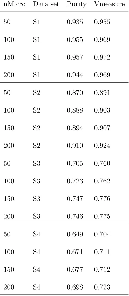
For the experiments in which the number of micro-clusters (q) and window size (w) is fixed, the value of the parameters must be selected. A brief computational study was carried out on a selection of simulated data sets for the purpose of parameter selection. Table 2.5.1 shows the Unweighted CluStream algorithm performance in terms of purity and V-measure for a number of parameter choices. The results are averaged over 10 runs. We can see that the performance improves as the number of micro-clusters increases, however, the performance seems to plateau aboveq = 150. Given that the computationally time increases linearly (see Section 2.4.1) q= 150 is a sensible parameter choice for the purposes of our study.

Now, we consider the choice of window size (w). Table 2.5.1 shows the windowed algorithm performance in terms of purity and V-measure for a number of parameter choices. Again,the results are averaged over 10 runs. We see that the performance improves marginally as the window size increases, however, the performance appears to be flat around w = 150 to

w= 200. As there is no advantage to using a window size greater than 150 we choose to set

(55)

[image:55.612.201.412.179.664.2]

Table 2.5.1: Select of nMicro parameter for CluStream.

nMicro Data set Purity Vmeasure

50 S1 0.935 0.955

100 S1 0.955 0.969

150 S1 0.957 0.972

200 S1 0.944 0.969

50 S2 0.870 0.891

100 S2 0.888 0.903

150 S2 0.894 0.907

200 S2 0.910 0.924

50 S3 0.705 0.760

100 S3 0.723 0.762

150 S3 0.747 0.776

200 S3 0.746 0.775

50 S4 0.649 0.704

100 S4 0.671 0.711

150 S4 0.677 0.712

(56)

[image:56.612.187.427.177.664.2]

Table 2.5.2: Selection of window size parameter for windowed algorithm.

Window Size Data set Purity Vmeasure

50 S1 0.928 0.957

100 S1 0.912 0.952

150 S1 0.922 0.959

200 S1 0.916 0.955

50 S2 0.872 0.903

100 S2 0.889 0.912

150 S2 0.898 0.918

200 S2 0.897 0.918

50 S3 0.741 0.779

100 S3 0.777 0.793

150 S3 0.794 0.804

200 S3 0.787 0.796

50 S4 0.69 0.723

100 S4 0.713 0.735

150 S4 0.726 0.738

(57)

2.5.4 Simulated Results

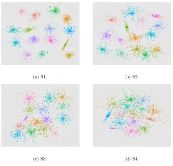
The first data sets tested are the popular S-sets, first introduced in Fr¨anti and Virmajoki (2006). The four data sets are shown in Figure 2.5.1.

(a) S1. (b) S2.

[image:57.612.130.485.162.503.2]

(c) S3. (d) S4.

Figure 2.5.1: The S sets (Fr¨anti and Virmajoki, 2006), two-dimensional data sets with varying degrees of overlap. The true clusters labels are shown.

(58)

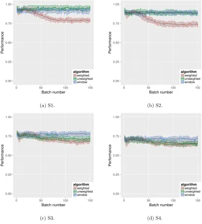
clustering to assign data points to clusters. Performance is evaluated in batch every 10th time point. The results are shown in Figures 2.5.2 and 2.5.3.

(a) S1. (b) S2.

[image:58.612.84.481.132.572.2]

(c) S3. (d) S4.

Figure 2.5.2: Purity for the S data sets.

(59)

shows the performance in terms of V-measure. Both figures show the algorithm performance at each batch step, meaning that we can see how performance changes as the data stream progresses. However, these data sets are stationary in distribution and therefore we would not expect to see algorithm performance vary dramatically with time.

(a) S1. (b) S2.

[image:59.612.84.485.189.628.2]

(c) S3. (d) S4.

Figure 2.5.3: V-measure for the S data sets.

(60)

perform similarly for all sets. They both perform well on set S1 and set S2 but they struggle with the more challenging sets S3 and S4. The weighted spectral CluStream (red) initially starts with performance on par with the competing algorithms, but quickly drops to poor performance and does not recover as the stream progresses. Given that the underlying distributions for the S sets are stationary, this behaviour is unusual.

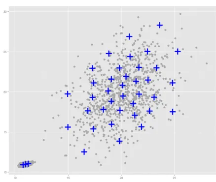
[image:60.612.154.453.310.524.2]

In order to discover why weighted spectral CluStream is performing poorly, lets look at the micro-clusters more closely. Figure 2.5.4 shows a snapshot of the weighted spectral CluStream algorithm on the S1 data set in the middle of the stream.

Figure 2.5.4: Snapshot from weighted spectral CluStream on S1.

(61)

This implies that the affinities between the micro-cluster centres on the outskirts of the cluster C are more similar to the outliers of other clusters (such as cluster I) than to the micro-cluster centres at C. This behaviour is very odd and implies that there might be an issue with the affinity matrix.

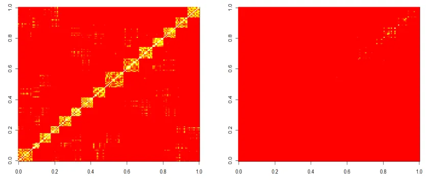
We can observe the affinity matrix by plotting it as an image, where bright values imply an affinity value close to one and red means the value is close to zero. Figure 2.5.5 shows an image of both the unweighted and weighted affinity for the example shown in Figure 2.5.4. The affinity matrix has dimension 150×150, with each row representing the similarities between one micro-cluster centre and the other 149. The rows and columns have been grouped so that micro-cluster centres from the same true underlying clusters are next to each other.

[image:61.612.97.514.379.562.2]

(a) Unweighted affinity matrix. (b) Weighted affinity matrix.

Figure 2.5.5: Affinity matrices for S set 1.

(62)

micro-clusters making this an informative affinity matrix to use with spectral clustering. However in the weighted affinity matrix (Figure 2.5.5b) the block nature is not visible. Most of the values are close to zero, with only a few strong affinities. The weighting seems to have dampened the affinity matrix, incorrectly reducing the affinity of close micro-clusters. It is possible that the use of the localised scaling parameter (see Section 2.2.2) in the spectral clustering step may be interfering with the weighting of micro-clusters. We did attempt to use a global scaling parameter instead of the localised one, however this then brought up the issue of tuning the σ parameter, which is known to be very sensitive and is a difficulty for spectral clustering algorithms in general (von Luxburg et al., 2008). Although performance did seem to improve with the global scaling parameter when chosen carefully, the performance was still very poor compared to windowed spectral clustering and spectral CluStream.

2.5.5 Texture data

(63)

[image:63.612.81.501.66.248.2]

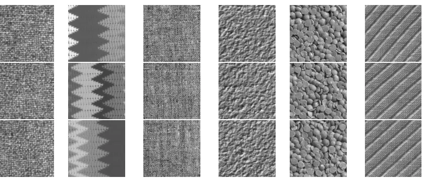
Figure 2.5.6: Three examples from each of the 6 different texture tiles. The texture classes are (L-R) Blanket 1, Blanket 2, Canvas, Ceiling, Lentils and Screen.

A subset of 6 classes was selected, examples of which are shown in Figure 2.5.6. The classes selected are images of two types of blanket, some canvas, a ceiling, some lentils and a screen. The performance plots for the texture data are shown in Figure 2.5.7. Here we do see a difference between windowed spectral clustering and unweighted spectral CluStream, the windowed approach is generally performing better. Once again weighted spectral CluStream does not perform well, and performance declines as the stream progresses.

(64)

[image:64.612.76.538.72.319.2]

(a) Texture Purity. (b) Texture V-measure.

Figure 2.5.7: Texture Results.

2.5.6 Pendigit data

(65)

(a) PCA of digits 1 and 6.

(b) Purity digits 1 and 6. (c) V-measure digits 1 and 6.

(d) PCA of digits 4 and 7.

[image:65.612.67.500.73.423.2]

(e) Purity digits 4 and 7. (f) V-measure digits 4 and 7.

Figure 2.5.8: Pendigits Pairwise - spectral CluStream and windowed spectral clustering.

Efficient analysis of data streams