and Actuator Networks
Jose Manuel Linares
Cert Web Apps (Open), BSc Open (Open), BSc Computing (Hons) (Sund)
School of Computing and Communications
Lancaster University
This dissertation is submitted for the degree of
Master of Philosophy
I would like to start this dedication in memory of four of my family relatives who have
passed away since I have been here conducting my research in Lancaster from 2012 to 2017.
In memory of:
• Concepción (Puri) Viagas
• Francisca Rumbo
• Dr. Bernard Linares
• Amalia Rumbo Martinez
Two of my family members succumbed to Cancer (Amalia and Bernard) and a sum of £612
was raised for Cancer Research UK in 2015 and cycled Wrynose or Bust 115 mile
cyclo-sportive challenge and a 65 mile reliability ride The Coal Road Challenge run by The
Lune Road Cycle Club. Thank you to the Lancaster Rotary Club for organizing the Wrynose
I would like to thank the following as they have supported me in my success either
directly or indirectly
To the late Dr. Harry Erwin who supported and convinced me to go for a PhD whilst I was
studying Computing at Sunderland University. I’m not there yet, but I’ll get there one day.
Dr. F. Taiani, who accepted me in this project in 2012 and supervised me until late 2012. It
was a pleasure to have met you.
Darren Grech and others from the Gibraltar Department of Education for understanding the
difficulties that I have had in this project and providing me the economic support when I
needed it the most. You also taught me A level Computing during 1997/1998 alongside with
Mr. Mañasco and this was the first step towards my development in Computer Science.
Ben Green, the conversations we had over the years were insightful and kept me going with
this project. Please look after the "joesterizer" RTU prototype.
Dr. Gerald Kotonya, for providing much needed assistance and understanding.
Dr. Phil Benachour, without him, I would have left Lancaster long before writing this thesis
My pet dog Frank the Pug, who has always kept me company on my long nights typing
away, a dog is really a man’s best friend.
Lastly, I would like to dedicate this to Georgina Garcia, she is always supportive of me and
without her, I doubt this work would have been completed - I love you.
I would like to end this dedication with a quote which is fitting to this body of research as
there were many unforeseen challenges along the way. I hope it will serve as an inspiration
for those considering doing a research degree. Doing research is akin like running a
marathon or participating in an arduous cyclo-sportive; there will be many challenges and
obstacles ahead and you have to pace yourself to reach the finishing line. Perseverance and
resilience will pay dividends.
"After climbing a great hill, one only finds that there are many more hills to
climb"
I hereby declare that except where specific reference is made to the work of others, the
contents of this dissertation are original and have not been submitted in whole or in part
for consideration for any other degree or qualification in this, or any other university. This
dissertation is my own work and contains nothing which is the outcome of work done in
collaboration with others, except as specified in the text and Acknowledgements. This
dissertation contains fewer than 65,000 words including appendices, bibliography, footnotes,
tables and equations and has fewer than 150 figures.
Jose Manuel Linares
I would like to acknowledge my first main supervisor Dr. F. Taiani who supervised me in my
research for the first ten months of my project and my replacement main supervisor, Prof.
Utz Roedig, for taking on the responsibility of supervising me. Brendan O’Flynn, you have
given me the feedback needed which I have dedicated many hours in amending the final
version of this thesis.
Lastly, I acknowledge Mr. Ben Green, who allowed me to use his test bed on the B floor
[4B] Four Bit
[ACK] Acknowledgement
[AHP] Analytical Hierarchy Process
[AI] Artificial Intelligence
[AT] Attention
[ARQ] Automatic Repeat Request
[ATEX] Appareils destinés à être utilisés en ATmosphères EXplosives
[CMOS] Complimentary Metal Oxide Semiconductor
[CSI] Channel State Information
[CSO] Combined Sewage Overflows
[DTU] Disruption Tolerant Networking
[DUCHY] Double Cost Field Hybrid Link
[EWMA] Estimated Window Moving Average
[ETX] Expected Transmission Count
[FFEWMA] Flip-Flop Estimated Window Moving Average
[FFPLSI] Flip-Flop Packet Loss and Success Interval
[FIS] Fuzzy Inference System
[FISPI] Fuzzy Inference System Pi
[FISCOM] Fuzzy Inference System Communication
[FISCORE] Fuzzy Inference System Core
[FISAI] Fuzzy Inference System Artificial Intelligence
[FRB] Fuzzy Rule Base
[GLONASS] Global Navigation Satellite System
[GPS] Global Positioning System
[GSM] Global System for Mobile Communications
[ISM] Industrial, Scientific and Medical Band
[KLE] Kalman Link Estimator
[LAN] Local Area Network
[LI] Link Inefficiency
[LQE] Link Quality Estimator
[LQI] Link Quality Indicator
[LUSTER] Light Under Shrub Thicket for Environmental Research
[MADM] Multiple Attribute Decision Making
[MANET] Mobile and Adhoc Networks
[OFCOM] Office of Communications
[PDR] Packet Data Reception
[PRR] Packet Reception Rate
[PSR] Packet Success Rate
[RH] Relative Humidity
[RNP] Required Number of Packets
[RSSI] Received Signal Strength Indicator
[RTU] Remote Terminal Unit
[SCADA] Supervisory Control and Data Acquisition
[SSA] Signal Stability Based Adaptive
[TCP] Transmission Control Protocol
[TWMA] Time Weighted Moving Average
[UHF] Ultra High Frequency
[VHF] Very High Frequency
[WiFi] Wireless Fidelity
[WMEWMA] Window Mean Exponential Weighted Moving Average
[WPAN] Wireless Personal Access Networks
This thesis will provide an insight on how weather factors such as temperature, humidity
and air pressure affects radio links and use this body of knowledge to better understand
how to mitigate unnecessary radio switching to take place and then use this knowledge
to suggest ways of developing a Link Quality Estimator that utilize online weather data
to be able to conduct smart link switching. In the context of this thesis, we focus on the
case study of a water utility company as these entities are under increasing economic and
environmental pressures to optimise their infrastructure, in order to save energy, mitigate
extreme weather events, and prevent water pollution. One promising approach consists in
using smart systems. However, a smart infrastructure requires reliable communication links
which are difficult to provide. In particular, communication links that are distributed and
geographically located in rural areas are highly affected by changing weather conditions,
hence efficient control of these distributed hosts requires robust communications. Multiple
communication transceivers are used to mitigate this issue and to enable nodes to switch to
reliable links. Short-term link quality estimators are used to decide which link to use which
often leads to the situation where a link switch is initiated which does not prove helpful in the
long term. It is not beneficial to switch a link and associated routing for only a brief duration
hence we conduct test bed experiments to better understand the relationships between the
radio links and weather factors and use this body of data to devise a LQE that can use this
List of figures xxi
List of tables xxv
1 Introduction 1
1.1 Chapter Overview . . . 2
1.2 Motivation . . . 2
1.3 Contribution . . . 3
1.4 Structure of Document . . . 4
1.5 Background . . . 4
1.5.1 Wastewater Systems . . . 5
1.5.2 Fuzzy Logic Control . . . 7
1.5.3 Wireless Communications for Waste Water Networks . . . 11
1.6 Chapter Summary . . . 12
2 Related Work 13 2.1 Link Quality Estimators . . . 13
2.1.1 Hardware Based LQE’s . . . 14
2.1.2 Software Based LQE’s . . . 16
2.1.3 Link Inefficiency (LI) . . . 23
2.3 Link Selection Schemes . . . 31
2.4 Proposed Weather Based LQE Using RSSI and Weather Data . . . 33
2.5 Options For Radio Nodes . . . 35
2.6 Chapter Summary . . . 36
3 Meteorological Effects on Wireless Links 37 3.1 Chapter Overview . . . 37
3.2 Weather Factors . . . 37
3.2.1 Temperature . . . 38
3.2.2 Humidity . . . 38
3.2.3 Air Pressure . . . 38
3.2.4 Experimental Setup . . . 39
3.3 Test Bed Experiment between Infolab21 and Galgate . . . 42
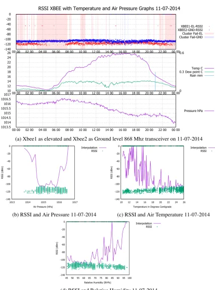
3.3.1 Ground And Elevated Placements . . . 43
3.3.2 Summary On July 2014 Data Collection . . . 92
3.4 Observable Effects On 868 Mhz Link . . . 94
3.5 Observable Effects On GSM Band . . . 99
3.6 Chapter Summary . . . 99
4 Weather Based Link Selection Scheme 101 4.1 Chapter Overview . . . 101
4.1.1 Short Term Link Quality Estimators . . . 101
4.1.2 Long Term Link Quality Estimators . . . 102
4.1.3 Link Selection Using Short and Long Term LQEs . . . 106
4.2 Processing of Data and Parameter Discovery . . . 107
4.2.1 Simulation Data Processing . . . 107
4.2.3 Finding Optimal Values . . . 108
4.3 Evaluation . . . 114
4.4 Results And Optimization Problem . . . 118
4.4.1 August 2015 . . . 121
4.4.2 UK Storms in 2015 . . . 121
4.4.3 Weather Based LQE Results in November and December 2015 . . . 124
4.5 Chapter Summary . . . 130
5 Prototyping, deploying and evaluating open architecture RTU 133 5.1 Chapter Overview . . . 133
5.2 Implementation Of RTU . . . 133
5.2.1 Requirements . . . 134
5.2.2 Hardware Components . . . 134
5.2.3 Assembly Of RTU . . . 140
5.2.4 Test Bed Used For Testing RTU . . . 142
5.2.5 Software Utilized - FISPI And Other Libraries . . . 144
5.3 Communication Component FIS COM . . . 148
5.4 Evaluation Testbed . . . 148
5.4.1 Performance Of The RTU . . . 149
5.4.2 Challenges In Developing The RTU . . . 149
5.5 Chapter Summary . . . 150
6 Conclusions 151 6.1 Chapter Overview . . . 151
6.2 The Problem Presented In This Thesis . . . 151
6.3 The Proposed Hypothesis . . . 152
6.4.1 Test Bed Platforms Developed . . . 154
6.4.2 Experiments Carried Out . . . 154
6.4.3 Results Obtained . . . 155
6.4.4 Analysis Of Results . . . 156
6.5 Future Work Recommendations . . . 157
6.5.1 Evaluating the Hardware Energy Efficiency of the RTU Build . . . 157
6.5.2 FIS COM Performance With Weather Based LQE . . . 157
6.5.3 Simpler And Efficient FISALG Module . . . 157
6.5.4 Using Parameters From Previous Months For LQE . . . 158
References 159
Appendix A Data Sheets 163
1.1 Schematic of a wet well . . . 6
1.2 Anglian Water’s energy costs (£60m) . . . 7
1.3 Fuzzy membership functions . . . 9
2.1 Four bit LQE diagram from Fonseca et al [19]. Arrows pointing outwards rep-resents information the estimator requests from the layers. Arrows pointing inwards represents the information that the layers provide . . . 21
2.2 Structure of DUCHY [39]. . . 23
2.3 Experimental setup in Bannisters’ paper [12]. . . 26
2.4 Loss due to Temperature [12]. . . 26
2.5 Maximum Range Vs Temperature [12]. . . 27
2.6 RSSI and LQI falling as temperature rises [14]. . . 28
2.7 LUSTER deployment in Hog Island [25]. . . 29
2.8 Exploiting weather data to predict packet drops [25]. . . 30
3.1 Air Pressure diagram showing low and high regions . . . 40
3.2 Experimental test bed map . . . 41
3.3 Experimental test bed radio box . . . 42
3.4 Test bed layout between University campus area and Galgate . . . 43
3.6 Analysis during the 07-07-2014 applying best line fit . . . 48
3.7 Analysis during the 08-07-2014 applying best line fit . . . 50
3.8 Analysis during the 09-07-2014 applying best line fit . . . 52
3.9 Analysis during the 11-07-2014 applying best line fit . . . 54
3.10 Analysis during the 12-07-2014 applying best line fit . . . 56
3.11 Analysis during the 13-07-2014 applying best line fit . . . 58
3.12 Analysis during the 14-07-2014 applying best line fit . . . 60
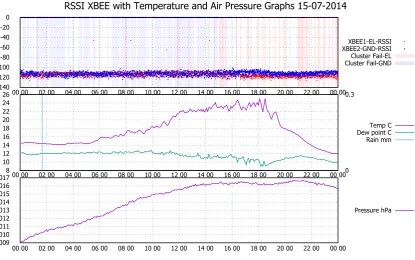
3.13 Analysis during the 15-07-2014 applying best line fit . . . 62
3.14 Analysis during the 16-07-2014 applying best line fit . . . 64
3.15 Analysis during the 17-07-2014 applying best line fit . . . 66
3.16 Analysis during the 18-07-2014 applying best line fit . . . 68
3.17 Analysis during the 19-07-2014 applying best line fit . . . 70
3.18 Analysis during the 20-07-2014 applying best line fit . . . 72
3.19 Analysis during the 21-07-2014 applying best line fit . . . 74
3.20 Analysis during the 22-07-2014 applying best line fit . . . 76
3.21 Analysis during the 23-07-2014 applying best line fit . . . 78
3.22 Analysis during the 24-07-2014 applying best line fit . . . 80
3.23 Analysis during the 26-07-2014 applying best line fit . . . 82
3.24 Analysis during the 27-07-2014 applying best line fit . . . 84
3.25 Analysis during the 28-07-2014 applying best line fit . . . 86
3.26 Analysis during the 29-07-2014 applying best line fit . . . 88
3.27 Analysis during the 31-07-2014 applying best line fit . . . 91
3.28 June 16th 2014 graph . . . 95
3.29 May 24th 2014 graph . . . 96
3.30 Dec 10th 2014 weather bomb graph . . . 97
4.2 Simulation run during July 2014 . . . 119
4.3 Simulation run during July 2014 - zoomed in . . . 120
4.4 Simulation run during August 2015 . . . 122
4.5 November 2015 period from the 1st to the 17th November . . . 128
4.6 December 2015 period from the 1st to the 5th December . . . 129
4.7 Storm Desmond - Lancaster Flooded . . . 131
4.8 Storm Desmond Weather Station Output . . . 132
5.1 OsiSense Analog Ultrasonic sensor. . . 135
5.2 Xbee Pro 868 Mhz series 5. . . 136
5.3 Raspberry Pi model B Rev 2. . . 136
5.4 Gertboard. . . 137
5.5 Euro card used to interface with the gertboard and external devices. . . 138
5.6 RAS clock. . . 138
5.7 A photo of the switch bottom left, DC to DC booster on the right and the RTU.139
5.8 RTU Front Panel. . . 141
5.9 RTU Inside Front Panel. . . 142
5.10 Inside the RTU. . . 143
5.11 Test Bed used to test the RTU and algorithm. . . 144
5.12 Switches for the pumps and separate power source for ultrasonic sensor. . . 145
5.13 FISPI architecture. . . 146
5.14 FISPI data encapsulation. . . 146
A.1 Gertboard schematic diagram. . . 163
A.2 Raspberry Pi R2 GPIO pinouts. . . 164
A.3 Xbee Pro 868 Mhz series radio transceiver used in our test bed experiments. 165
A.4 Xbee Pro 868 Mhz series 5 data sheet. . . 166
B.1 Simulation run during November 2014 . . . 176
B.2 Simulation run during December 2014 . . . 177
B.3 Simulation run during March 2015 . . . 178
B.4 Simulation run during April 2015 . . . 179
B.5 Simulation run during September 2015 . . . 180
4.1 Parameters assigned to the S + L LQE . . . 103
4.2 May 2015 Sub Optimal values . . . 110
4.3 May 2015 Sub Optimal values 2 . . . 110
4.4 May 2015 optimal . . . 111
4.5 May 2015 Sub Optimal values 3 . . . 113
4.6 May 2015 Optimum values . . . 113
4.7 July 2014 based on figure 4.2 . . . 116
4.8 July 2014 . . . 116
4.9 June 2015 using May 2015 parameters . . . 117
4.10 June 2015 Sub Optimal values 1 . . . 117
4.11 June 2015 Optimal Parameters . . . 118
4.12 August 2015 OP . . . 121
4.13 August 2015 Sub Optimal values . . . 123
4.14 Beaufort Scale . . . 124
4.15 2015 UK storms . . . 124
4.16 November Sub Optimal Values 2015 . . . 126
4.17 November Optimal Values 2015 . . . 126
4.18 December SubOptimal Values 2015 . . . 127
B.1 September 2014 . . . 169
B.2 November 2014 . . . 170
B.3 November 2014 . . . 170
B.4 March 2015 . . . 171
B.5 April 2015 . . . 171
B.6 May 2015 standard 2 . . . 172
B.7 May 2015 - 2 . . . 172
B.8 June 2015 standard . . . 173
B.9 June 2015 - 2 . . . 173
B.10 June 2015 equal weights . . . 174
B.11 September 2015 . . . 174
Introduction
In most developed countries, water infrastructures and services play a critical role in
protect-ing the public health, and preventprotect-ing damages to human and natural environments. Water
infrastructures are well known for delivering drink-water, but they also play a key role in
providing irrigation to agriculture, limiting water-based pollution, and mitigating extreme
weather events such as floods and droughts. Managing, maintaining, and updating these
infrastructures is, however, costly and complex. Water infrastructures are heavily distributed
(over several 10,000 km2 in some instances), include a large range of equipment (pipes,
pumps, sewers, vanes, treatment plants, controllers), and have often been constructed over
several decades, sometimes going back as far as Victorian times (1837 - 1901).
As environmental regulations are developed, water consumption surges (mainly due to
population growth), and energy costs rise, water companies are under increasing pressure
to update and improve the management of their infrastructure. One promising plan is in
using better control systems (“smart” systems) to reduce operational costs and improve
services. Such systems rely on control theory (fuzzy logic, decision trees), wireless sensors
and actuators networks (WSANs), and better models to achieve their aims. Unfortunately, in
spite of some promising starts [18, 42], few of these systems are deployed in production today.
tailored towards the water industry where each wet well can handle communications between
other pumping stations and control its own pumps to prevent localised flooding.
1.1
Chapter Overview
In this chapter, the motivations for this project will be highlighted with the contributions made,
then proceed in outlining how this document is structured. We then give a background of
how waste water industries generally work but specific to one company who we co-operated
with. We give examples of such control algorithm to control inputs and outputs that can be
applied to a Remote Terminal Unit (RTU), and lastly, describe present and future wireless
communications within the waste water industry. We then give a brief summary of what was
discussed in this chapter.
1.2
Motivation
It is limiting to work with Remote Terminal Unit’s (RTU’s) that utilize closed architecture
systems due to their closed nature in terms of gaining access to the source code used for
specific hardware. Most of these systems work at high voltages of 12V in order to make
switches to actuators possible. Hence it is desirable for researchers in this field to build an
open architecture that can be easily replicated and can be easily replaced with ubiquitous
off-the-shelf components that are available in specialized electronic stores making it easy to build,
maintain, cheap to build and less demanding in terms of voltage use than the proprietary 12V
RTU. Hence we will outline how to build an RTU that is an open architecture, inexpensive to
build and utilizing software that has a vibrant community of developers.
Therefore, a possible solution would be to integrate a communication platform that
can address these difficulties that current systems have at the moment. We can address
solution would be to use cheaper long range radio transceivers (for e.g. 868 Mhz range) to
communicate with sensor nodes. Unfortunately this too faces challenges as meteorological
environments do impact radio quality. A possible way of building a communication platform
is by integrating different existing technologies together. In brief, we need the following to
make a communication platform:
1) A control algorithm (fuzzy logic as an example) to decide when actuator switches
should take place and react on sensed data from sensors, in our case, it will be water levels.
2) A hardware open platform to be able to integrate our code and test it appropriately for
our evaluation.
3) An understanding of how weather affects radio communications and explore ways of
how transceiver switches can be done.
1.3
Contribution
The contribution in this thesis is explained as follows on the three points below:
1) To better understand how meteorological aspects affect radio link quality, explore
how it is possible to reduce radio interface switching and suggest how a new Link Quality
Estimator can be built utilizing online meteorological data. This contribution would provide
a better understanding on the relationships that meteorological factors play when carrying
out switching.
2) Design a Link Quality Estimator (LQE) based on the data provided from the first
contribution to reduce costly switching (Evil Switching).
3) Using the LQE developed to make smart link switching.
To carry out these contributions, we therefore need to have a test bed that collects RSSI
data, packet drops and weather data to better understand the relationship between radio links
1.4
Structure of Document
The structure of this thesis is divided into 6 chapters. The first chapter gives an introduction
to the problem that this thesis addresses and its motivation, it describes how this thesis
contributes to a unique body of knowledge giving a brief introduction of Link Quality
Estimators. In chapter 2, we give an overview and discussion on related work on link quality
estimators, link selection algorithms and meteorological effects on wireless propagation. In
chapter 3, we give a introduction on the meteorological factors and data we collect, explain
how these factors are related to each other and show our observations on how these have
affected our test bed. In chapter 4, we discuss the strengths and weaknesses of current Link
Quality Estimators and explain why we need a new link quality estimator that relies on
externally available weather data. In chapter 5, we describe the prototype RTU that was
developed for our case scenario and give an overview of the test bed used, ending with an
evaluation of communication performance and a conclusion in chapter 6.
1.5
Background
In this section, we give an overview of how waste water infrastructures operate, how are such
infrastructures controlled, why do these infrastructures require communications and the need
for an open platform Remote Terminal Unit (RTU) to operate a bespoke control system as
described by our industrial partners in Anglia Waters Ltd. An RTU may be locally present
within a sub station, but its control algorithms may reside on another host located remotely
as there is a desire to move from a centralised topology into a hybrid distributed topology in
case there is a fault.
Waste water networks are complex infrastructures that combine civil engineering works
(sewers, basins, reservoirs), hydraulic actuators (pumps, gates, valves), sensors (water levels
control logic usage in waste water networks is very simple, often relying on fixed threshold
values to trigger behaviours (e.g. switching a pump on or off), but more advanced control
techniques are now being considered, with fuzzy logic proposing to be a promising candidate
[35]. In the context of Anglian Waters, they employed Fuzzy Logic in their system, we would
emphasise here that there are many types of control algorithms that can do the same task of
controlling actuators and sensing data although efficiencies will vary between algorithms
which require separate analysis. In the following, we describe in detail the structure and
constituents of a waste water network (Section 1.5.1). We then provide a quick introduction to
fuzzy logic, and explain how it applies to the control of waste water networks (Section 1.5.2).
1.5.1
Wastewater Systems
A waste water infrastructure is usually organised in catchments. Each sewer catchment
consists of a connected network of sewer pipes that collect sewage in an area and bring it
to a treatment plant or a discharge point. The number of catchments managed by a water
company can be substantial and, taken together, can cover an extensive area. Anglian Water
for instance collects waste water from about 6 million customers through 1,100 waste water
catchments over an area of 27,500 km2in the East of England.
Many sewer catchments use acombined sewer systemwhich collects both waste water
from households and storm water during rainfall. A combined sewer system must have
enough capacity to process a large range of water inflows. This large capacity is needed to
prevent toxic flooding in case of heavy waters (wet weather conditions), but also to avoid high
concentrations of toxic substances if the rainwater is insufficient (dry weather conditions).
Mere gravity is usually insufficient to transport water in a sewer catchment. A catchment
is therefore often equipped with a set of pumping stations that transport waste water over an
!"#$%&'()*)('
+,-./0"1)'(,%)'
2,1/'-)301)'304)"'()*)('
5#3'-)301)'304)"'()*)('
6)4'3)((' 74#"8'9$89'
:--,-4
'
9$89' [image:32.595.176.458.129.348.2]+$4;'9$89'
Fig. 1.1 Schematic of a wet well
A pumping station is built around a wet well (Figure 1.1), an underground reservoir that
acts as a buffer for incoming water from a main sewer pipe. A wet well is usually equipped
with 2 to 3 pumps: aduty pump, anassist pumpand, in some critical wet wells, astorm pump
(see [35] for more details of pumps).
The pumps of a wet well can be switched on and off, and must be controlled to process
the incoming water, while minimising energy consumption, and optimising the pumps’
lifetime. The opportunities for energy consumption are substantial, as energy costs constitute
a substantial part of the operational budget of most water companies [35]. Anglian Water for
instance spends about £60 million pounds in energy costs annually, with £32 million being
spent on waste water operations, of which £9 million allocated for waste water networks
(Figure 1.2). Similarly, unexpected pump failures can have drastic consequences, possibly
leading to the flooding of pollutants. Finally, although this is rarely implemented at the
1.5 Background 7
Other energy costs £37M
!"#$%&'()*&
+,-"$.,"$%&
/$".0%1-&'2*&
+,-"$.,"$%&
"%$,"3$/"&
'4(*&
Fig. 1.2 Anglian Water’s energy costs (£60m)
known asCombined Sewer Overflows(CSO for short), which are tightly regulated, and can
carry heavy financial and environmental consequences.
A Combined Sewer Outage occurs when the capacity of a combined sewer system is
exceeded, usually as a result of heavy rainfall. Sewer networks are in this case, designed to
discharge some the excess water directly into the environment (river, lake or sea) without
treatment. A better management of pumps during (short) heavy rainfall could in principle
mitigate CSO by better utilising the buffer capacity of wet wells.
1.5.2
Fuzzy Logic Control
In this subsection, we describe one of many possible types of control algorithms that may
be implemented into an RTU. A control algorithm is needed to carry out actuator controls
of pumps and receive inputs on water levels so that the RTU can react to constant changes
in levels. This particular method of using fuzzy logic was researched by Dr.Ostojin from
Sheffield University who were part of the Anglia Water Ltd research project. Dr.Ostojin et
reduces maintenance costs [35]. Other methods of control algorithms exist, but this was
chosen by the sponsor.
In spite of the potential benefits of better control in combined sewer systems, most
pumping stations are handled today by a basic logic, embedded in a Programmable Logic
Controller (PLC) installed in the station. The PLC uses input from ultrasonic sensors to
activate each of the pumps according to hard-coded water levels [35].
Any improvement on this basic approach should fit the needs of the water industry: It
should have a low total cost of ownership, due to the large number of pumping stations to be
equipped (Anglian Water for instance manages approximately 4,500 pumping stations which
have 12,500 pump sets all together); it should be robust for unexpected events and failures;
and should be easily portable to different stations with little deployment and tuning efforts.
Principles Of Fuzzy Logic
Fuzzy logic meets most of these needs, and is one of the solutions currently researched by
Anglian Water [35]. Fuzzy logic extends traditional Boolean logic with continuous truth
values between 0 (false) and 1 (true), rather than just 0 and 1. In control, a fuzzy logic
approach usually starts by afuzzyfication step, in which the inputs of the control system
are processed through a set of fuzzy membership functions [23, 32]. For instance, if one of
the inputs is the water level in the wet well, Figure 1.3 shows the truth value of the three
fuzzy predicatesLOW_LEVEL,MEDIUM_LEVEL, andHIGH_LEVEL. For a water level of
1.25 meters, the truth value ofLOW_LEVELis 0.75, that ofMEDIUM_LEVELis 0.25 and that
ofHIGH_LEVELis 0.
The control part of a fuzzy-base control logic typically takes the form offuzzy rule-based
inference systems, FRB for short. An FRB uses a set of if-then rules to encode the actions
the system should take, depending on its input predicates, for instance:
1.5 Background 9
Other energy costs £37M
Water level low_level medium_level high_level
0 1 0 0
1 1 0 0
2 0 1 0
3 0 0 1
4 0 0 1
!"#$%&'()*&
+,-"$.,"$%&
/$".0%1-&'2*&
+,-"$.,"$%&
"%$,"3$/"&
'4(*&
5& 5647& 567& 56)7& 8&
5& 8& 4& (& 9&
!"#$%&'
()#*&
+($*"&)*'*)&,-*$*"./&
:0.;:$<$:& 3$=>?3;:$<$:& #>@#;:$<$:&
Fig. 1.3 Fuzzy membership functions
Theifparts (the antecedent) of all rules are evaluated in parallel, using a fuzzy semantic
for Boolean operators (e.g. xandyis usually interpreted asmin(x,y)). The resulting truth
values are then used to compute thethenpart (consequent) of each rule, in a way that differs
depending on the type of FRBs considered.
In the simplest case (known as Mamdani FRBs), the consequent and antecedents are used
to determine a fuzzy membership function for the whole FRB through animplicationand an
aggregationstep. This function computes how the truth value of the whole system varies
with the output variables (in our case the switching states of the pumps) for the observed
input (the water level).
The final stage consists then of transforming this system-wide membership functions into
actual control values (which pumps to switch on/off), known as thedefuzzyficationstep. This
last step usually seeks to maximise the average truth value of the system, while taking into
account the many-value logic captured by the FRB.
Although all FRB follow the above steps (fuzzyfication,implication,aggregation,
defuzzy-fication) variations point are numerous. First, Mamdani inference systems are only one type
of FRBs, with Tagani-Sugeno FRBs another important alternative. Tagani-Sugeno FRBs use
directly provide an output value for control. Within the Mamdani family itself, many variants
exists depending on the semantic of the fuzzy operators (maxbeing one option only forand
for instance), and the detail of the aggregation and defuzzyfication steps.
Besides the above design choices, the quality of control delivered by an FRB strongly
depends on the design of its input membership functions. Here again several approaches
exist. A basic approach consists in relying on expert knowledge. More advanced strategies
are however often taken that use optimisation to search for an optimal set of membership
functions maximising particular quantities (energy consumption, pump lifetime, risk of
CSOs). This optimisation usually occurs off-line using historical data, but recent works
have been proposed to optimise membership functions dynamically based on the system’s
feedback [41].
Fuzzy Logic At Anglian Water
Anglian Water have started experimenting with fuzzy-logic to optimise the energy
consump-tion of one pumping staconsump-tion in dry weather condiconsump-tion [35]. The approach uses a Mamdani
FRB to switch the pumps of the wet well on and off depending on the wet well’s water
level, the flow of water coming in, and the current electricity tariff (night or day). The input
membership functions are configured off-line on historical data using a genetic algorithms to
optimise the energy consumption, while minimising pump switching (a factor of premature
wear).
This early system was shown to deliver energy saving of between 2 and 2.5%, a promising
start which is now being refined by Anglian Water (at present, it is over 6% with matlab
simulations). Unfortunately the latest development in a real setting has not been able to
produce the energy saving envisaged and thus, the company has asked for the advice of
Lincoln University on other methods of control which may be less complex (such as IF
1.5.3
Wireless Communications for Waste Water Networks
Control algorithms are required to sense data from sensors to detect water levels and send
signals to actuators to activate or deactivate pumps. In the previous section, we described the
fuzzy logic that was employed within Anglia Water’s test bed. We re-iterate here that fuzzy
logic is one of several types of control algorithms and this is an active research area that is
being conducted at other Universities (Sheffield and Lincoln). Anglia Waters Ltd is one of
the largest water companies in the UK, part of their problem was due to utilizing GSM radio
during periods of stormy weather. Their implementation was to have a contract GSM SIM
card where each pumping station can send data wirelessly. This means that data needs to be
transported through the network provider’s infrastructure which may have some latency. This
can be costly to the company but also depends on which contract plan there are available
specifically for industrial purposes.
One solution they found was to implement an OFCOM licensed 150Mhz (VHF) point to
point system which can carry a signal to a range of over 20 miles. This solved the company’s
initial problem, but at an annual cost of over £8000 per year to have that band protected.
An envisaged wireless future is to use similar radio implementations but at a higher
frequency such as 433 Mhz or 868 Mhz radio frequencies. We selected the 868 Mhz
frequency as it is currently available and free to use radio band and some hardware devices
were available at the time. The hardware implementation used is Xbee series 5 which has its
own proprietary mesh protocol, but it is possible not to use it and have a generic or specialised
protocol programmed in the host instead.
In our scenario, a future of decentralised sub stations would be able to communicate with
each other running a middleware platform where software modules may be remotely located
and not necessarily present locally should failure occur. Instead of control being sent over
a SCADA centralised network, we would have a hybrid decentralised system, capable of
transmitted to another wet well for decisions to be taken or b) locally managed by the wet
well host.
1.6
Chapter Summary
We have given an overview as to why resilient communications is needed within waste water
networks and given an overview of how these systems operate. We have also given an idea
of one possible way of controlling inputs and outputs via a control algorithm. We give an
overview of what fuzzy logic is and why it was used in this context. We ended the chapter
by giving an overview of how present and future communication infrastructures would look
like within the waste water industry either by utilizing licensed radio frequencies, or utilize
Related Work
In this chapter, we discuss the related work that is based on Link Quality Estimators that have
been surveyed and tested in a real outdoor environment setting similar to our test bed, Link
Quality Selection and the impact that meteorological factors have, such as air temperature,
relative humidity and air pressure has on links and link quality estimators.
2.1
Link Quality Estimators
In this subsection, we will cover the different types of related work that encompasses Link
Quality Estimators. Fundamentally, a Link Quality Estimator provides a service to higher
communication protocols that would mitigate link unreliability at the physical level, thus
ensuring that the routing layer maintains good links and provide a stable topology.
Link Quality Estimators (LQE) can be categorised as either hardware or software based
schemes. Software based LQE’s are further subdivided into three categories, Packet
Recep-tion Rate (PRR) based, Required Number of Packets (RNP) based and Score based. Software
LQE’s can provide more fine grain control [10] and are able to monitor link quality for certain
applications that might involve indoor monitoring applications or outdoor applications that
2.1.1
Hardware Based LQE’s
These types of LQE’s include the received signal strength (RSSI), Link Quality Indicator
(LQI) which is available on certain nodes and Signal to Noise Ratio (SNR). These LQE’s are
read from the radio transceiver and an advantage of hardware LQE’s over software LQE’s
is that there is no further computations required, thus saving CPU cycles and saves energy
which is beneficial to an energy limited node.
Received Signal Strength Indicator
In RSSI, the RSSI register is the received power of a connected region of the last received
packet and it does not look into the correctness or quality of the signal [3]. The RSSI value
is not standardised across the physical hardware to the RSSI reading; for example, 802.11
WiFi standard does not define a relationship between milliwatts (mW) or decibel milli watt
(dBm) [2]. Generally, the closer the value is to 0, the better the received signal will be; as an
example, -50 dBm has a greater received signal power than -80 dBm. We state that in our
work, a value of 0 means a dropped packet and not an excellent RSSI signal strength.
Liu et al noticed in his work that different vendors and even devices from the same vendor
will differ in RSSI levels [29], thus RSSI has a limitation to be used to measure distances in
Wireless Local Area Networks.
A single reading can determine if the link is within the transitional region according to
Baccour [10] although it is not possible to determine an RSSI value if the packet was not
received .
Srinivasan et al [28], states that link estimation is important when designing new protocols
based on RSSI, as he stated in his work that there is a wide belief in the Wireless Sensor
Network community that RSSI is a bad estimator. His motivation for his work was based in
the assumption that older generation radio motes such as the MicaZ, Telos and Intel Mote 2
asymmetric links; one radio node may have a link but the other radio node does not have
enough range. In Srinivasan’s work [28], he shows that the CC2420 chipset has a low or
insignificant miscalibration due to symmetric link between nodes. The CC2420 chipset has a
reliable RSSI indicator when it is above a sensitivity threshold of -87 dBm [28]. When this
threshold is broken, it does not have a correlation with Packet Reception Rate (PRR) and
it is believed that this is due to local noise variations at different nodes. Srinivasan states
that protocol designers looking for cheap and agile link estimators might consider RSSI over
Link Quality Indicator (LQI).
Signal to Noise Ratio (SNR)
Signal to Noise Ratio is the difference between the pure signal strength and the level of
background noise floor at the receiver [10]. According to Srinivasan [44], SNR metrics will
be better than RSSI readings as noise floor across different nodes differ. An observation that
Aguayo et al [8], Senel et al [43] and Yunqian et al [30], showed that there are difficulties
in establishing relationships between SNR and PRR, thus SNR cannot be used alone as
an estimator as this depends on the actual hardware sensor as environmental effects like
temperature [43] has an effect on the sensor hardware.
Link Quality Indicator (LQI)
LQI is a metric that is used to measure signal quality and is an estimate on how a signal can
be demodulated (extraction of data from an analogue signal to a digital signal) by acquiring
the magnitude of errors between motes that have good links and the received signal over the
64 symbols (a symbol is a waveform such as a tone when transmitting via a modem or a
pulse in digital baseband transmission which represents a number of bits) after the sync word
LQI is a proposed standard for IEEE (2003) 802.15.4 but is vendor specific [10]; the
CC2420 chipset which is a widely available chip, utilizes LQI in this manner. This metric is
measured on the first 8 symbols (a symbol can be conveyed as either a single bit of data or
several bits of data) of the received packet as a score which ranges from 50 which is a low
quality link to 110 which is good quality link. However, Srinivasan [28] argues that LQI
is not a good predictor for intermediate quality links due to its high variance (due to that it
is a statistical value) unless it is averaged over some time with several readings, however,
it is preferred that LQI is averaged over a larger window of packets (40 to 120 packets) to
determine if the link is of good quality but sacrificing agility and responsiveness in changes.
2.1.2
Software Based LQE’s
In this sub section, we shall give an overview of the popular types of Link Quality Estimators
that have been tested in a real smart grid setting for an electric utility company by Gungor et
al [21]. These LQE’s have also been evaluated in a survey by Baccour et al [10] who has
given some results albeit some are indoors whereas we are more concerned on real outdoor
environment experiments done by Gungor et al [21] as the application is similar to our test
bed and intended application area.
Packet Reception Rate (PRR)
Packet Reception Rate or PRR, is a simple metric that was widely used in routing protocols
and it is a receiver based LQE that calculates the average rate of packets received on the
receiver node [10]. The shorter the window is to calculate the average, the more accurate
it can be in predicting failures, but at the cost of network stability as failure could be for
a short time caused by external factors such as interference or moving objects. Under the
PRR category, we will look into Window Mean Exponential Weighted Moving Average
Weighted Mean (WMEWMA)
The Window Mean Exponential Weighted Moving Average is a simple LQE algorithm that
is measured as the percentage of packets that have been received on the receiver side intact
[46] [10].
In Woo’s work [46], he ran a test bed using Berkely motes which use the 916 Mhz band
and running over the TinyOS operating system. He used a single sender generating packets
which are sequenced over a rate of 8 packets per second. The receiver node then redirects
these packets over a serial port to a PC where these are stored. By looking at the sequence
numbers, Woo was able to calculate packet losses by using success/loss events over time
and packet success rates over time as the fraction of packets that were received over the 30
second interval. The nodes were placed indoors and outdoors but within short distances of
15 feet which is approximately 4.5 metres.
In WMEWMA or Window Mean Exponentially Weighted Moving Average, Woo uses a
low pass filtering by taking the average of a time window and adjust the estimation using
the latest estimation. The computed average success rate over a time period is smoothed
with and exponentially weighted moving average. This LQE takes in two parameters; the
first is time and the second is the history size of the estimator. It also takes in two tuning
parameters; time and history size of the estimator. The estimator however does require a
minimum number of packets before it can make a link quality estimation.
In Woo’s experiments [46], there was observable results when an obstruction was placed
(a person) in between the two nodes with a distance of 8 feet where packet probability was
0.8 to 0.6 without an obstruction and then dropped down to 0 when the obstruction was
present. Packet probability oscillated between 0.5 and 0.8 when there was no obstruction.
Therefore, there is a need to address this problem by designing a link estimator that can track
these changes in an agile and responsive way which is simple and uses little computational
variations. In Woo’s work, he lays out the different types of agile estimators suited ideally
for multi hop routing.
One candidate is Estimated Window Moving Average or EWMA were Woo et al, [46]
used this estimator to compare it with other link estimators since it is widely used. In EWMA,
the algorithm requires constant storage of the old estimates to be able to do any fine tuning.
EWMA uses linear combination of infinite history that are weighted exponentially, thus this
makes the algorithm reactive to small shifts and it is considered an agile detector in many
statistical process control applications.
In Woos’ work, [46], it is suggested that the Flip-Flop EWMA is the best estimator to
provide agility and stability by Kim et al [26] since statistical theory is used to select the best
estimator. Woo explored the possibility of using Flip Flop-EWMA by setting the agile and
stable EWMA tunings to be the same as in the EWMA study [46]. There are two methods in
setting this estimator; the agile method can be set as default and make the estimator switch to
the stable estimator when there is a 10% difference in noise margin. The other approach is to
make the stable estimator as default but as soon as disturbances are detected, it will switch to
the agile estimator when estimations deviate by 10%. However, it is shown in Woo’s paper
[46] that Flip-Flop EWMA does not provide an advantage over the much simpler EWMA in
his test bed because fluctuations in the agile estimator are so bad, it will introduce instability
and errors and criticises Kim’s work [26] as to why Flip-Flop EWMA is better in his test
bed as it does not show the dynamics of either estimator in a separate way over time. Other
estimators taken into consideration are Moving Average, Time Weighted Moving Average
(TWMA) and Flip-Flop Packet Loss and Success Interval with EWMA (FFPLSI) all which
underperform WMEWMA.
Woo’s conclusion is that WMEWMA outperforms other forms of estimations since it
100 packet times. WMEWMA is ideal for resource constrained devices since the storage
requirement is constant for all tunings.
Kalman Filter (KLE)
Software based schemes such as Kalman filter (KLE) [43] estimates PSR (Packet Success
Rate) by adjusting PSR-SNR relationships which gives an indication to the link quality
although it must be stated that accuracy was not examined in Baccour’s survey [10] and the
KLE filter was tested in controlled indoor environments which delivered consistent results.
This LQE was devised to overcome the poor reactivity of average based LQE’s such as PRR.
Essentially, it provides link quality estimation based on the received signal strength of one
packet. It is unnecessary to wait for several packets in order to compute a value. As soon as
it receives a packet, this packet is transferred to the Kalman filter which outputs an estimate
of the received signal strength. An output of the Signal to Noise Ratio (SNR) which is the
KLE representation is computed by subtracting the noise floor (the sum of all non-man made
and man-made interference) estimate from the estimated received signal strength and then
using a pre-calibrated PRR-SNR (Packet Reception Ratio - Signal to Noise Ratio) curve at
the receiver node, the approximated SNR is mapped to an approximated PRR.
Required Number Of Packets (RNP)
RNP is a sender-side estimator that takes into account the number of transmissions and
retransmissions needed before the node successfully receives it [10]. The RNP is calculated
by the window of transmitted or retransmitted packets divided by the number of successfully
received packets minus one to exclude the first packet sent. This LQE assumes an automatic
repeat request (ARQ) protocol at the link layer which will send retransmissions of a packet
until it is correctly received at the other node end. Under the RNP category, we look into
Expected Transmission Count (ETX)
The ETX scheme by Couto et al [16] was developed to take into account lossy links and
find paths with the highest throughput despite how long the link may be, requiring several
hops to reach its destination. In his paper [16], he took measurements from a wireless
test bed using 29 nodes consisting of Linux PC with a Cisco/Aironet 340 PCI 802.11b
card with a 2.2 dBi dipole antenna and showed that ETX can find routes that yield higher
throughputs rather than using a minimum hop count metric. Several improvements have been
proposed in the protocol development such as prediction of loss ratios for varying packet
sizes, handling of networks that run on different bit rates and making ETX more robust
when handling high levels of data traffic. The ETX was developed to be an improvement
from the existing minimum hop count metric as it does not take into consideration that
longer paths may yield higher throughputs. ETX is an active monitoring LQE scheme on the
receiver side which is calculated by computing the loss ratio between the two directions of
each link and interference caused from outside sources taking into account link asymmetry
(electromagnetic radio propagation not being completely spherical in shape). It is argued that
ETX is ideal for Mobile and Adhoc Networks (MANETs) due to mobility, but not true in a
static Wireless Sensor Network (WSN) deployment where Four bit out performs ETX on
its own as it relies on the 802.15.4 Level 2 acknowledgements (ACKs) to measure the ETX
[39], [19].
Four Bit(4B)
Four bit LQE in essence is a hybrid estimator developed by Fonseca et al [19] where link
failure is monitored by amalgamating 4 bits of data from different network layers that exist in
most hardware interfaces. Fonseca’s argument in developing four bit (referred in his paper as
layer which uses 4 bits of data to tell if the link is reliable, or unreliable by using existing
[image:47.595.220.387.171.326.2]layers that can provide useful data to the LQE.
Fig. 2.1 Four bit LQE diagram from Fonseca et al [19]. Arrows pointing outwards represents information the estimator requests from the layers. Arrows pointing inwards represents the information that the layers provide
The Fourbit LQE takes 1 bit from the physical layer, 1 bit from the link layer and 2 from
the network layer. The white bit is taken from the physical layer which denotes channel
quality and can determine good or bad links. The acknowledge (ACK) bit taken from the
link layer indicates whether an acknowledgement is received for a sent packet. The last two
pieces of data are the pin and compare bit which are read from the network layer and are used
to build the neighbour node tables for routing purposes. It then combines two link metrics
which is the ETX for unicast packets (window size divided by number of acknowledged
unicast packets). The second metric is the beacon packet which is calculated by applying an
EWMA average of the window size, divided by the number of received beacons. These two
metrics are then combined using a EWMA average.
Score based
In this subsection, score based Link Quality Estimators can be Channel State Information
Hybrid Link Estimators - DUCHY
A hybrid score based - CSI and Packet Data Reception (PDR) - LQE is DUCHY (Double
Cost Field Hybrid link estimator) developed by Pucinella et al, [39] designed for network
layer integration cost based protocols and was used over the Arbutus WSN routing protocol
[38]. DUCHY selects the routes with the shortest hops and the highest quality links and it is
based on two LQE’s; the first is the CSI which is a normalised value between the RSSI and
LQI which are collected from received beacons (see diagram 2.1.2) and then combines these
two normalised values into a weighted sum. The second LQE is the RNP (ETX) which is
used to refine CSI values which can be incorrect due to that these are based on beacon traffic.
DUCHY leverages on broadcast control traffic and unicast traffic and utilizes CSI and
delivery estimates (ETX) to address typical problems found in WSN’s such as weak signals
and to strengthen low quality links by coding and using ARQ or Automatic Repeat Request
(see diagram 2.1.2). The problem presented in [39] is that coding offsets the energy saving
that it should bring whereas ARQ’s are more commonly used and the problem in WSN nodes
is that they are usually static and if the channel of two nodes are in a deep fade, then it may
take an indefinite time for the fading pattern to change. Thus, lossy links will need many
retransmissions if no other alternative is available.
DUCHY does not require neighbourhood tables but keeps the state of the parent node.
RSSI is used to obtain information on good links and LQI is used to get information
about bad links. It also borrows from Fonseca’s idea [19] to use the L2 ACK’s for unicast
outgoing packets. The idea of DUCHY is specific to 802.15.4 since LQI although it could be
implemented in non 802.15.4 standard.
The most common form of Channel State Information LQE is RSSI as mentioned
previously and used to be considered a poor predictor due to limitations in the hardware [39]
and [50]. However, because developers focus on the 802.15.4 stack, they use the CC2420
Fig. 2.2 Structure of DUCHY [39].
In evaluating DUCHY, Baccour [10] states that Arbutus was compared to MultiHopLQI
(a hierarchical routing protocol based on LQI) as an LQE. In Puccinellis work [39], they
found that Arbutus outperforms MultiHopLQI and deduce that DUCHY is better. Baccour
argues that this is an unfair deduction due to that the two LQE’s were compared in different
contexts and suggested that it would be more reasonable to integrate LQI in Arbutus and
compare DUCHY based Arbutus to LQI based Arbutus [10]. However, DUCHY does
perform better than LQI because it integrates LQI and other estimator metrics and Baccour
ends the analysis, noting that it would be interesting to compare DUCHY and other software
LQE’s to demonstrate its performance.
2.1.3
Link Inefficiency (LI)
Link inefficiency is a Link Estimator designed by Lal et al [27] to save energy by taking
into consideration weak signals from neighbouring nodes by conducting a brief initialization
audit as soon as the radio transceivers are powered up. More data can then be collected
after this initialization phase. Although the test bed was conducted indoors during 7 days,
Lal used sensor node hardware from Bosch Research with an 8 bit microcontroller. The
915 Mhz ISM band. If nodes have the ARQ protocol employed, it would mean that the node
will send out a number of retransmissions until it has succeeded in sending the data packet
to the neighbouring nodes. Thus, the more retransmissions there are on a weak signal, the
less likely the packet will be sent and LI is modelled on how probable the data packet can be
delivered by using the least amount of energy. This is done by getting the RSSI for every byte
of data received and averaging the RSSI value for the complete data packet. The SNR was
also collected and used to determine if links are good or bad quality; in their test bed, if the
link is less than 15 dB, then it is considered a bad link. Lal also used Packet Success Rate or
PSR, to get the ratio between the good packets and bad packets over a 300 second time frame
where 3000 packets over 300 seconds would be a PSR of 100%. To determine link cost the
author [27] proposes that the channel SNR is sampled, if the SNR is below a pre-determined
threshold, the instantaneous link inefficiency as the reciprocal PSR is measured. If the SNR
is above the threshold, then LI is calculated by inverting PSR and weighed with the factor
that depends how away the threshold is from the ideal SNR. Then include the instantaneous
LI value in a running average for all samples taken. Lal has shown in his work that only a
few metrics are required to predict when links will fail and thus be able to take more data
into account as soon as the neighbouring nodes are up and running. In Baccour’s discussion
[10], it is noted that PSP is a form of approximated Packet Reception Rate (PRR) and was
shown by Aguayo [8], Yunqian [30], Senel [43] and Lal [27], that mapping from average
SNR to an approximation of PRR can lead to an erratic estimation, thus using PSP instead of
Non Traditional LQE’s
Other forms of hybrid LQE’s used involve the use of fuzzy logic [11] in determining link
quality, apply four bit in hardware implementations [19] or use mapping methods [43] to
determine link quality. Unfortunately, fuzzy processing does require a certain amount of
processing carried out by the node itself which its power source may be limited.
2.2
Environmental Effects on Radio Transceivers
In this section, we look at different types of wireless radio transceivers and examine what the
authors have researched in terms of how these are affected by external factors such as heat,
humidity and air pressure.
Bannister et al [12] studied the effects of temperature on Received Signal Strength, data
collection and localization. In his work, it was aimed to characterize the effect of temperature
on commercially available sensor nodes and to understand how it affects WSN deployments.
In Bannisters’ research, he used the IEEE 802.15.4 TI CC2420 Radio in a Tmote sky wireless
mote. The CC2420 datasheet [5] discusses how temperature can affect the internal oscillator,
however in the CC2400 datasheet [4], does include graphs of the output power and receiver
sensitivity over an operating range.
Bannister sets up two motes to observe the effect that temperature has on RSSI. To
eliminate noise from external sources, he connects both motes using a coaxial cable and a
sequence of attenuators - see figure 2.2. The temperature inside the chamber started from
an initial temperature of 45 °C and then rising to 65 °C before allowing it to cool down and
then remained for a 45 minute period. The temperature was measured using the on-board
Sensirion SHT11 sensor. The power readings were collected by averaging the RSSI over a 10
power of 0 dBm. Each mote was swapped as transmitter and receiver and inside and outside
[image:52.595.147.416.472.693.2]of the temperature chamber to see observable effects.
Fig. 2.3 Experimental setup in Bannisters’ paper [12].
It was found that there is a loss in RSSI of 8 dB at 65 °C. A linear pattern was found
to express the relationship between RSSI and temperature and it is presented in Bannisters’
paper. He states in his paper that there is already work done previously that temperature
decreases the efficiency of Radio Frequency (RF) circuitry [4], [47] [49].
The increase of temperature at 65 °C has a negative impact on range as seen in figure
2.2 as it shows a 4 dBm to 5 dBm decrease in output from the transmitter and 3 dBm
decrease in measured input power by the receiver for approximately 8 dB decrease combined.
Communication range is also affected as can be seen in figure 2.2 when 65C is when there is
[image:53.595.168.435.251.474.2]a significant loss in range than operating in a 45C environment.
Fig. 2.5 Maximum Range Vs Temperature [12].
Thus by using a linear model function, it is possible to state a Log-Distance Path Loss
Model to estimate the effect of temperature on the maximum communication range between
two sensor nodes. Bannister concludes that this is not a malfunction of the circuitry that
measures the RSSI but it effectively corresponds to a decreased ability for the radio to
demodulate signals with low power and his findings is consistent with the findings of Wu,
et al, [47] where temperature is shown to decrease the efficiency of the low noise amplifier
stage in a Complementary Metal Oxide Semi-Conductor (CMOS) receiver.
In 2010, Boano et al [14], explores how ambient temperature affects an oil refinery WSN
using the 802.15.4 stack and the 2.4 Ghz ISM band. In an experiment to quantify how heat
affects the motes, the sender and receiver mote were cooled to between -15 °C and -3 °C and
then heated up to 50 °C in 90 minutes whilst sending data packets with a 12 byte payload
every 4 seconds. The motes are separated 3 metres apart and transmission power is kept at
-3 dBm throughout the experiment. The result from this experiment is that both sender and
receiver had a loss of 4 dBm to 5 dBm in three separate runs - see figure 2.2. Tests were
also conducted by placing the same motes inside ATEX compliant boxes to observe if heat
affected the motes inside. The result of having motes inside ATEX compliant boxes is that
temperature will be warmer inside the box than outside the box. It was observed that RSSI
decreased as temperature increased.
Fig. 2.6 RSSI and LQI falling as temperature rises [14].
In 2013, Boano et al [13] tried to quantify how temperature can dramatically reduce radio
throughput. In his work, Boano attempts to design a low cost experimental infrastructure
(WisMotes employing CC2520 and CC2420 using the ZigBee 802.15.4 stack at 2.4 Ghz ISM
band) to vary the temperature of the low power transceiver in a repeatable and predictable
manner. It was found that temperature can affect all platforms in the same way; in radio
transceivers, it leads to a reduction of SNR which leads to a lower link quality and a shorter
Thelen et al investigated the effect of radio propagation for two months on a potato field
utilizing Chipcon CC1000 radio transceivers using the Mica2Dot 433 Mhz version [45].
Relating to our studies, Thelen concludes that foliage does affect radio propagation and limits
range to 10 metres, but radio waves propagate better in conditions that are high in humidity,
especially at night and when raining. Thelen did dismiss the fact that the curvature of the
Earth has no effect due to that the range between the radio nodes is very limited (up to 50
metres). This is in contrast to work done by Anastasi et al who used the 868 Mhz version
and found that the presence of fog and rain decreased transmission range significantly [9].
Kang et al [25], wrote a paper which is based on WSN deployments in Hog Island, USA,
under a project named LUSTER (Light Under Shrub Thicket for Environmental Research)
and describes a long range setup (see figure 2.2), were WSN nodes powered by solar energy,
sends data packets back to the main server over several kilometres using Gain antennas.
Fig. 2.7 LUSTER deployment in Hog Island [25].
One of the problems Kang described in the paper is that wind had a noticeable effect in
packet drops and thus, Kang et al developed a delay/disruption-tolerant networking (DTN)
technique as retransmitting data which were lost via the network would be lost due to wind.
The reason highlighted in the paper that wind affects this deployment is due to the size of the
antennas are used. Hence a weather aware DTN technique was developed to avoid the WSN
to send data when there were wind speeds exceeding a particular threshold. In the discussion,
it is highlighted that publicly available weather data was used to predict when outages may
occur and hence delay transmission until wind speeds are more tolerable. Results were
recorded and plotted on graphs seen in figure 2.2 where in a) is the wind level of the week
and was observed that wind speed is strong between February 5th and February 10th. Plot b)
reveals failure rates are much greater than in plots c) and d) where wind speeds at 15mph
mitigates less packet drops than in plot d) which mitigates packet drops at lower threshold of
wind speeds reaching 10 mph.
Fig. 2.8 Exploiting weather data to predict packet drops [25].
In Kang’s paper, rain, fog and snow did not have any noticeable effects in their setup
radio operation under 10 Ghz frequency bands does not have an effect on rain, snow or fog.
However, it is documented that a build-up of snow has a negligible effect as this degrades the
sensitivity of the antenna.
In Hall’s et al paper [22], work was done with Very High Frequency (VHF) and Ultra
High Frequency (UHF) to confirm if anticyclonic weather conditions affects positively the
range of radio signals. In his experiment, Hall used two trans horizon radio paths, the first
radio path was 114 Km apart from Peterborough to Slough using a frequency of 90 Mhz and
the second radio path was from Crystal Palace in London to Peterborough which are 121 Km
apart using a frequency of 573 Mhz. Over a period of days from August to September in
1966, it was observed that during the night, there was an increment of 5 dB in signal power
and the author demonstrates in his paper using ray tracing techniques that during periods of
anticyclonic weather, abnormally high values of radio strength occurs at night and returns to
normal during the sunset. This phenomenon is due to radio signals being reflected from the
troposphere and down to the surface. To further explain the term anticyclonic, it is a region
of high pressure that pushes cold air downwards to the surface from the upper atmosphere
to the surface causing good weather. The effect of air pressure and anticyclonic weather is
explained in more detail in section 3.2.3.
2.3
Link Selection Schemes
In this section, we look at previous related works in link selection algorithms.
Dube et al [17] proposed the Signal Stability Based Adaptive (SSA) routing protocol
in MANETs due to the problem that in a dynamic network, fast changes in routing tables
can cause nodes to have tables that are out of date and inaccurate and the constant changing
topology would cause problems in looping routes. Dube et al performed simulations to show

![Fig. 2.1 Four bit LQE diagram from Fonseca et al [19]. Arrows pointing outwards representsinformation the estimator requests from the layers](https://thumb-us.123doks.com/thumbv2/123dok_us/9374444.440110/47.595.220.387.171.326/diagram-fonseca-arrows-pointing-outwards-representsinformation-estimator-requests.webp)
![Fig. 2.3 Experimental setup in Bannisters’ paper [12].](https://thumb-us.123doks.com/thumbv2/123dok_us/9374444.440110/52.595.147.416.472.693/fig-experimental-setup-in-bannisters-paper.webp)
![Fig. 2.5 Maximum Range Vs Temperature [12].](https://thumb-us.123doks.com/thumbv2/123dok_us/9374444.440110/53.595.168.435.251.474/fig-maximum-range-vs-temperature.webp)