Hyperspectral Band Selection Using Improved
Classification Map
Xianghai Cao,
Member, IEEE,
Cuicui Wei, Jungong Han,
Member, IEEE
Licheng Jiao,
Senior Member, IEEE
Abstract—Although it is a powerful feature selection algorithm, wrapper method is rarely used for hyperspectral band selection. Its accuracy is restricted by the number of labeled training samples and collecting such label information for hyperspectral image is time consuming and expensive. Benefited from the local smoothness of hyperspectral images, a simple yet effective semi-supervised wrapper method is proposed, where the edge preserved filtering is exploited to improve the pixel-wised classi-fication map and this in turn can be used to assess the quality of band set. The property of the proposed method lies in using the information of abundant unlabeled samples and valued labeled samples simultaneously. The effectiveness of the proposed method is illustrated with five real hyperspectral datasets. Compared with other wrapper methods, the proposed method shows consistently better performance.
Index Terms—Hyperspectral image, band selection, semi-supervised, wrapper method, filtering
I. INTRODUCTION
R
EMOTE images collected by hyperspectral sensors oftencapture hundreds of bands for each pixel and each land cover type has unique reflection characteristics for these spectral bands. This sort of spectral information is very useful for distinguishing different land cover types. However, due to the Hughes phenomenon [1], high dimensionality sometimes brings negative effect. Usually, feature extraction and feature selection are two widely used methods that conquer this problem.
Feature extraction often produces new features by linearly or nonlinearly combing the original features. Huang et al. [2] used structure feature set to extract the statistical features of direction-lines histogram. Bandos et al. [3] analyzed the classification of hyperspectral images with linear discriminant analysis in the presence of a small ratio between the number of training samples and the number of spectral features. More recently, Li et al. proposed a multiple-feature learning classification method [4], which integrates multiple types of features extracted from both linear and nonlinear transforma-tions and has the ability to find both linear and nonlinear class boundaries presented in the data. In [5], feature selection and feature extraction were combined to improve the accuracy
This work is supported in part by the National Natural Science Foundation of China under Grant 61401322 and Grant 61405150, and in part by the Fundamental Research Funds for the Central Universities No. JB160222. (Corresponding author: Jungong Han.)
X. Cao, C Wei and L. Jiao are with Key Laboratory of Intelligent Perception and Image Understanding of Ministry of Education, International Research Center for Intelligent Perception and Computation, Xidian University, Xian, Shaanxi Province 710071, China.
J. Han is with the School of Computing and Communications, Lancaster University, LA1 4YW, UK.
of base classifiers. In this paper, feature selection is used to improve the classification accuracy of hyperspectral image.
Differently, feature selection selects some distinctive and discriminative bands to improve the performance of hyper-spectral image classification. Depending on the availability of labeled samples, feature selection can be categorized into supervised method, unsupervised method and semi-supervised method. The supervised method uses label information to assess the quality of each band. In [6], rough set theory was used to compute the relevance and significance of each spectral band. Then, by defining a novel criterion, it selects the informative bands that have higher relevance and significance values. The unsupervised method often selects representative bands based on the characteristics of the original images. A dual clustering approach was proposed for hyperspectral band selection in [7]. Wang et al. [8] proposed a saliency based band selection algorithm which puts the band vectors in the manifold space and treats the saliency problem from a rank-ing perspective. [9] proposed an unsupervised band selection method based on the differences among neighboring bands by exploring an intermediary representation called spectral rhythm. With respect to the semi-supervised method, both the labeled and unlabeled samples are used for band selection. [10] first built a hypergraph model from all hyperspectral samples and a semi-supervised learning method was intro-duced to propagate class labels to unlabeled samples. A linear regression model with group sparsity constraint was then used for band selection. Bai et al. proposed a semi-supervised pair-wise band selection framework, in which an individual band selection process is performed only for each pair of classes [11].
Based on the relationship between a feature selection al-gorithm and the classifier used to infer a model, three major methods can be distinguished [12]: Filter method, which relies on the general characteristics of data and conducts the feature selection process as a preprocessing step independent on the classifier; Wrapper method, which evaluates a subset of features by training and testing a specific classification model; and Embedded method, wherein the search of optimal subset of features is built into the classifier construction.
collecting such label information for hyperspectral image is time consuming and expensive. Based on linear Support Vector Machine (SVM), [14] used wrapper method to assess the importance of each band. In order to improve the accuracy of the wrapper method, Cao et al. predicted the overall classification accuracy by using the statistical characteristics of pixel-wised classification map [15]. Ren et al. improved the wrapper method by randomly introducing some classified samples into training stage [16].
As is well known, increasing the number of labeled samples is an effective way to improve the accuracy of wrapper method. However, the labeling work is too expensive for remote image. Therefore, learning how to increase the number of labeled samples with less efforts is the key for the success of wrapper method. Inspired by the spectral-spatial classification method of [17], the edge-preserving filtering is adopted to improve the pixel-wised classification map. This improved map is then used as the pseudo-ground truth to assess the quality of hyperspectral band set.
II. SEMI-SUPERVISED BAND SELECTION USING IMPROVED
CLASSIFICATION MAP
In this section, an edge-preserving filter is introduced. This filter is employed to improve the pixel-wised classification map, which is eventually used to select discriminative bands.
A. Edge-preserving filter
Reducing noise has always been one of the standard prob-lems of the image analysis and processing community. Mean-while, it is also important to preserve the edges. Therefore, it is desirable to preserve important features, such as edges, corners and other sharp structures, during the denoising process. Many kinds of edge-preserving filters have been developed, such as bilateral filter [18] and anisotropic diffusion [19]. In this paper, the guided filter [20] is adopted to improve the classification map.
SupposeI is the guided image,pis the input image andq
is the output image. We assume thatqis a linear transform of
I in a window ωk centered at the pixelk:
qi=akIi+bk,∀i∈ωk (1) where qi and Ii are the ith pixel of q andI.ωk is a square
window with radius r and (ak, bk) are linear coefficients
assumed to be constant in ωk. By minimizing the following
cost function:
E(ak, bk) =
X
i∈ωk
((akIi+bk−pi)2+a2k) (2)
the solution of(ak, bk)can be obtained by the equation (3) and (4), where is used to penalize largeak.
ak =
1 |ω|
P
i∈ωkIipi−µkpk
σ2
k+
(3)
bk=pk−akµk (4)
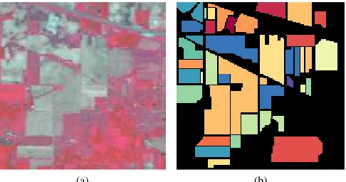
[image:2.612.317.560.65.193.2](a) (b)
Fig. 1. Indian Pines scene. (a) Three-band color composite image. (b) Ground truth.
Here, µk and σ2k are mean and variance of I in ωk, |ω| represents the number of pixels inωk. andpk is the mean of
pinωk. The filtered pixel can be computed by
yi =aiIi+bi (5)
where ai = |ω1|Pk∈ωiak and bi =
1 |ω|
P
k∈ωibk are the
average coefficients of every window including pixeli.
B. Improve classification map with edge-preserving filter
If there are enough labeled samples, wrapper based band selection will have satisfying accuracy. However, the high cost of obtaining labels makes it impractical in real applications. In this paper, the local smoothness of hyperspectral image is used to produce abundant reliable label information. For hyperspectral image, local smoothness means that neighboring pixels often share the same labels. Fig. 1 illustrates the Indian Pines dataset in which different colors represent different land cover types.
First, the SVM is used to produce the initial classifica-tion map. In this map, different numbers are used to rep-resent different land cover types. However, if this map is filtered directly, big numbers will get more weights than small numbers. Thus, the classification result is rewritten as
c= (c1, ..., cl, ...cL), in which ci,l indicates whether a pixeli
belongs to the lth class and cl has the same size with input
imagep. L is the total number of classes in the dataset. That is,
ci,l=
(
1 if pi∈l
0 otherwise (6)
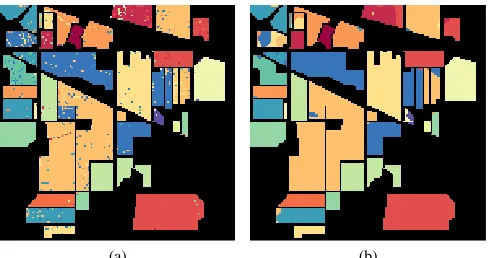
Initially, spatial information is not considered and the classi-fication maps appear noisy and not aligned with real object boundaries. To solve this problem, the classification maps are optimized by edge-preserving filtering. That is, eachcl is filtered by guided filter. Then, each pixel is labeled by finding
the maximum value of ci,l and the resulted classification
(a) (b)
Fig. 2. Indian Pines scene. (a) Classification map with SVM classifier. (b) Improved classification map with filtering.
C. Band selection based on the pseudo ground-truth
The accuracy of wrapper method is restricted by the limited label samples. Here, the pseudo ground truth is used to tackle this problem. Classic wrapper methods often use cross validation accuracy to select discriminative features, however, it is not suitable to use this strategy with the pseudo ground truth. Although pseudo ground truth is more reliable than pixel-wised classification map, it may still contain many wrong labels. If these wrong labels are used to train the classifier, this will degrade the performance of band selection. So, during the band selection, we train the classifier with labeled samples, then the pseudo classification accuracy of unlabeled samples can be calculated based on the pseudo ground truth.
The detailed band selection algorithm is summarized in Algorithm 1.
Algorithm 1 Band Selection Using Improved Classification Map (BS IC)
Inputs
- N band hyperspectral imageB={B1, B2, ..., BN}
- the selected band set Bs={ }
- the remaining band set Br={B1, B2, ..., BN}
1: With all band information, train an SVM classifier with labeled samples;
2: Label these unlabeled samples with this classifier; 3: Improve the classification map with guided filter and get the pseudo ground truth;
4: Combine each band image Bi inBr withBs;
5: Based on the combined image, train an SVM classifier with labeled pixels, then classify unlabeled pixels with this classifier and compute the classification accuracy based on the pseudo ground truth;
6: Choose the band Bm which has the highest accuracy, i.e.,
let Bs={Bs;Bm}, then remove Bm fromBr; 7: Jump to step 4, until the desired number of bands is obtained.
From the above description, we can see that BS IC is a semi-supervised wrapper method. Because the involvement of
classifier during band selection, and both the labeled and un-labeled samples provide useful information for band selection.
III. EXPERIMENT
In this experiment, five publicly available datasets are used to evaluate the performance of BS IC. For the guided filtering, the mean image over all bands is used as the guided image, and r is set as 5 for all datasets. For SVM classifier, the radial basis function (RBF) is used as the kernel function.
We adopt different strategies for the selection of C and γ:
during the band selection, the fixed values are used with
C = 1024 and γ = 2 to reduce the computation burden,
and these values are experientially determined; after the band selection, we use five-fold cross validation to choose the optimum parameters. Six band selection algorithms are used for comparison. Two unsupervised filter methods: Exemplars component analysis (ECA) [21] and volume gradient based band selection (VGBS) [22]. One supervised filter method: minimal redundancy maximal relevance criterion (mRMR) [23]. One classic wrapper method: SVMCV [24], i.e, wrapper method based on SVM classifier and cross validation. Two semi-supervised wrapper methods: Forward semi-supervised feature selection (Semiwrapper) [16] and wrapper method based on spatial information (Spatialwrapper) [15].
A. Indian Pines scene
This scene includes 16 land cover types, such as alfalfa, corn and woods. For this dataset, 10% labeled samples are used as training samples. Though 224 spectral bands were collected, only 200 bands are used for analysis after removing of water absorbed bands.
From Fig. 3 it can be observed that four wrapper methods show much higher accuracy than the other methods. Since Spatialwrapper and Semiwrapper are initialized with SVMVC. So, they always have the same accuracy with 10 selected bands. VGBS shows the worst performance, and mRMR and ECA exhibit similar performance. By introducing spatial information, Spatialwrapper and the proposed BS IC both obtained higher classification accuracy than classic SVMCV. In fact, the BS IC always obtains much better performance than Spatialwrapper with different band numbers. Semiwrap-per does not exhibit better Semiwrap-performance than SVMCV, because the high redundancy between selected features. When 10 and 100 bands are selected, the accuracy difference of BS IC and VGBS is 0.122 and 0.076, respectively. This result indicates that band selection can influence the classification accuracy remarkably.
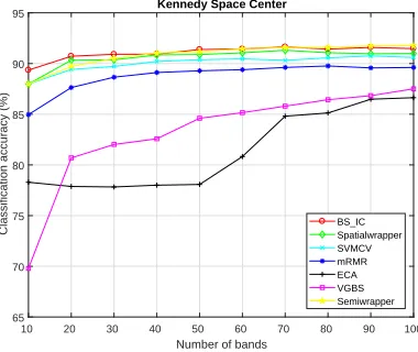
B. Kennedy Space Center (KSC)
[image:3.612.53.297.64.193.2]10 20 30 40 50 60 70 80 90 100
Number of bands
66 68 70 72 74 76 78 80 82 84 86
Classification accuracy (%)
Indian Pines
[image:4.612.341.532.62.222.2]BS_IC Spatialwrapper SVMCV mRMR ECA VGBS Semiwrapper
Fig. 3. Classification accuracy of Indian Pines scene.
10 20 30 40 50 60 70 80 90 100
Number of bands
65 70 75 80 85 90 95
Classification accuracy (%)
Kennedy Space Center
BS_IC Spatialwrapper SVMCV mRMR ECA VGBS Semiwrapper
Fig. 4. Classification accuracy of Kennedy Space Center.
Though ECA and mRMR obtain similar accuracy with Indian Pines scene, ECA shows much worse classification accuracy than mRMR with this dataset. This testifies that ECA is not a robust algorithm. BS IC still gets the best performance, although the Semiwrapper obtains a little high accuracy when band numbers exceed 80. Its classification accuracy is also robust with the different number of selected bands.
C. Botswana
This dataset was collected with Hyperion sensor at 30 m pixel resolution in 242 bands covering the 400-2500 nm portion of the spectrum. After preprocessing, uncalibrated and noisy bands that cover water absorption features were removed, and the remaining 145 bands were included as candidate features. For this dataset, 10% labeled samples are randomly selected as training samples.
The number of selected bands ranges from 5 to 50, and the classification results are plotted in Fig. 5. From this experiment, it can be seen that mRMR obtains much higher accuracy than classic SVMCV when the band number exceeds 15. The reason is that the accuracy of SVMCV is restricted by the limited labeled samples. When only 5 bands are selected, the classification accuracy of BS IC and mRMR is 0.884
5 10 15 20 25 30 35 40 45 50
Number of bands
74 76 78 80 82 84 86 88 90 92 94
Classification accuracy (%)
Botswana
[image:4.612.77.269.63.223.2]BS_IC Spatialwrapper SVMCV mRMR ECA VGBS Semiwrapper
Fig. 5. Classification accuracy of Botswana.
5 10 15 20 25 30 35 40 45 50
Number of bands
68 70 72 74 76 78 80 82 84
Classification accuracy (%)
Pavia University
BS_IC Spatialwrapper SVMCV mRMR ECA VGBS Semiwrapper
Fig. 6. Classification accuracy of Pavia University scene.
and 0.742, respectively. When 50 bands are selected, the classification accuracy of BS IC and mRMR is 0.925 and 0.911. This result testifies again that BS IC is more robust to the number of selected bands.
D. Pavia University scene
This scene was acquired by the Reflective Optics System Imaging Spectrometer (ROSIS). The number of spectral bands is 103. This scene has a high spatial resolution of 1.3 me-ters. For this dataset, we only select 1% labeled samples to train the classifier. Fig.6 shows that the ECA gets the lowest accuracy. The mRMR obtains similar performance with SVMCV, this testifies again that the accuracy of SVMVC is restricted by the limited labeled samples. However, with the local spatial information, Spatialwrapper improves the performance effectively. The proposed BS IC still posts the highest accuracy with different band numbers. However, the Semiwrapper shows much worse performance for without considering the redundancy between the selected bands.
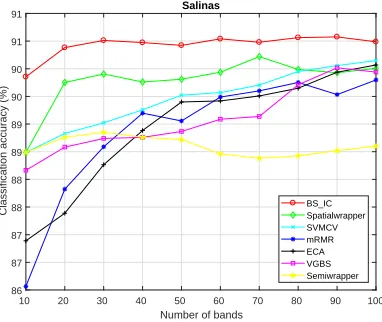
E. Salinas scene
[image:4.612.341.530.266.426.2] [image:4.612.78.268.267.427.2]resolu-10 20 30 40 50 60 70 80 90 100
Number of bands
86 87 87 88 88 89 89 90 90 91 91
Classification accuracy (%)
Salinas
[image:5.612.78.269.62.223.2]BS_IC Spatialwrapper SVMCV mRMR ECA VGBS Semiwrapper
Fig. 7. Classification accuracy of Salinas scene.
tion is 3.7 meters. The area covered comprises 512 lines by 217 samples. Similar to the Indian Pines scene, we discarded 20 water absorption bands. Overall, 1% labeled samples are used for training and the rest are earmarked for the test. For this dataset, as shown in Fig. 7, the performance difference of different algorithms is much smaller than other datasets. For example, when 10 bands are selected, the accuracy difference between BS IC and mRMR is only 0.038, whereas for KSC, the biggest accuracy difference is 0.196. Even so, the proposed BS IC still exhibits superior performance with different band numbers. This result demonstrates again that BS IC is a robust and effective band selection algorithm.
IV. CONCLUSION
Wrapper method is a powerful tool used to select discrim-inative bands. However, its accuracy is highly restricted by the limited labeled samples. For hyperspectral image, labeling work is expensive and time consuming, fortunately, the unique local smoothness makes the use of abundant unlabeled samples possible. Based on the local smoothness, a simple semi-supervised wrapper method is proposed in this paper. Its performance is much better than classic wrapper method by introducing the information of abundant unlabeled samples. Besides, our wrapper method is robust to the label noise [25], because the pseudo ground truth includes some noise labels. In the future, our wrapper method can be applied to select the binary features [26] and RGBD features [27].
REFERENCES
[1] G. P. Hughes, “On the mean accuracy of statistical pattern recognizers,”
IEEE Transactions on Information Theory, vol. 14, no. 1, pp. 55–63, 1968.
[2] X. Huang, L. Zhang, and P. Li, “Classification and extraction of spatial features in urban areas using high-resolution multispectral imagery,”
IEEE Geoscience and Remote Sensing Letters, vol. 4, no. 2, pp. 260– 264, 2007.
[3] T. V. Bandos, L. Bruzzone, and G. Campsvalls, “Classification of hyperspectral images with regularized linear discriminant analysis,”
IEEE Transactions on Geoscience and Remote Sensing, vol. 47, no. 3, pp. 862–873, 2009.
[4] J. Li, X. Huang, P. Gamba, J. M. Bioucas-Dias, L. Zhang, J. Atli Benediktsson, and A. Plaza, “Multiple feature learning for hyperspectral image classification,”IEEE Transactions on Geoscience and Remote Sensing, vol. 53, no. 3, pp. 1592–1606, 2015.
[5] J. Xia, N. Falco, J. A. Benediktsson, J. Chanussot, and P. Du, “Class-separation-based rotation forest for hyperspectral image classification,”
IEEE Geoscience and Remote Sensing Letters, vol. 13, no. 4, pp. 584– 588, 2016.
[6] S. Patra, P. Modi, and L. Bruzzone, “Hyperspectral band selection based on rough set,”IEEE Transactions on Geoscience and Remote Sensing, vol. 53, no. 10, pp. 5495–5503, 2015.
[7] Y. Yuan, J. Lin, and Q. Wang, “Dual-clustering-based hyperspectral band selection by contextual analysis,”IEEE Transactions on Geoscience and Remote Sensing, vol. 54, no. 3, pp. 1431–1445, 2016.
[8] Q. Wang, J. Lin, and Y. Yuan, “Salient band selection for hyperspectral image classification via manifold ranking,”IEEE Transactions on Neural Networks, vol. 27, no. 6, p. 1279, 2016.
[9] L. C. B. D. Santos, S. J. F. Guimaraes, and J. A. D. Santos, “Efficient unsupervised band selection through spectral rhythms,” IEEE Journal of Selected Topics in Signal Processing, vol. 9, no. 6, pp. 1016–1025, 2015.
[10] X. Bai, Z. Guo, Y. Wang, Z. Zhang, and J. Zhou, “Semisupervised hyperspectral band selection via spectralspatial hypergraph model,”
IEEE Journal of Selected Topics in Applied Earth Observations and Remote Sensing, vol. 8, no. 6, pp. 2774–2783, 2015.
[11] J. Bai, S. Xiang, L. Shi, and C. Pan, “Semisupervised pair-wise band selection for hyperspectral images,” IEEE Journal of Selected Topics in Applied Earth Observations and Remote Sensing, vol. 8, no. 6, pp. 2798–2813, 2015.
[12] V. Boloncanedo, N. Sanchezmarono, and A. Alonsobetanzos, “A review of feature selection methods on synthetic data,”Knowledge and Infor-mation Systems, vol. 34, no. 3, pp. 483–519, 2013.
[13] L. Ma, M. Li, Y. Gao, T. Chen, X. Ma, and L. Qu, “A novel wrapper approach for feature selection in object-based image classification using polygon-based cross-validation,”IEEE Geoscience and Remote Sensing Letters, vol. PP, no. 99, pp. 1–5, 2017.
[14] A. Le Bris, N. Chehata, X. Briottet, and N. Paparoditis, “Use inter-mediate results of wrapper band selection methods: A first step toward the optimisation of spectral configuration for land cover classifications,”
Proc. of the IEEE WHISPERS, vol. 14, 2014.
[15] X. Cao, T. Xiong, and L. Jiao, “Supervised band selection using local spatial information for hyperspectral image,” IEEE Geoscience and Remote Sensing Letters, vol. 13, no. 3, pp. 329–333, 2016.
[16] J. Ren, Z. Qiu, W. Fan, H. Cheng, and P. S. Yu, “Forward semi-supervised feature selection.” inAdvances in Knowledge Discovery and Data Mining, Pacific-Asia Conference, PAKDD 2008, Osaka, Japan, May 20-23, 2008 Proceedings, 2008, pp. 970–976.
[17] X. Kang, S. Li, and J. A. Benediktsson, “Spectralspatial hyperspectral image classification with edge-preserving filtering,”IEEE Transactions on Geoscience and Remote Sensing, vol. 52, no. 5, pp. 2666–2677, 2014. [18] C. Tomasi and R. Manduchi, “Bilateral filtering for gray and color images,” in International Conference on Computer Vision, 1998, pp. 839–846.
[19] P. Perona, “Scale-space and edge detection using anisotropic diffu-sion,”IEEE Transactions on Pattern Analysis and Machine Intelligence, vol. 12, no. 7, pp. 629–639, 1990.
[20] K. He, J. Sun, and X. Tang, “Guided image filtering,”Pattern Analysis and Machine Intelligence, IEEE Transactions on, vol. 35, no. 6, pp. 1397–1409, 2013.
[21] K. Sun, X. Geng, and L. Ji, “Exemplar component analysis: A fast band selection method for hyperspectral imagery,”IEEE Geoscience and Remote Sensing Letters, vol. 12, no. 5, pp. 998–1002, 2015.
[22] X. Geng, K. Sun, L. Ji, and Y. Zhao, “A fast volume-gradient-based band selection method for hyperspectral image,”IEEE Transactions on Geoscience and Remote Sensing, vol. 52, no. 11, pp. 7111–7119, 2014. [23] H. Peng, F. Long, and C. Ding, “Feature selection based on mu-tual information criteria of max-dependency, max-relevance, and min-redundancy,”Pattern Analysis and Machine Intelligence, IEEE Transac-tions on, vol. 27, no. 8, pp. 1226–1238, 2005.
[24] I. H. Witten, E. Frank, and M. A. Hall,Data Mining: Practical Machine Learning Tools and Techniques (Third Edition). Morgan Kaufmann Publishers Inc., 2011.
[25] T. Liu and D. Tao, “Classification with noisy labels by importance reweighting,” IEEE Transactions on Pattern Analysis and Machine Intelligence, vol. 38, no. 3, pp. 447–461, 2016.
[26] Y. Guo, G. Ding, L. Liu, J. Han, and L. Shao, “Learning to hash with optimized anchor embedding for scalable retrieval,”Image Processing, IEEE Transactions on, vol. 26, no. 3, pp. 1344–1354, 2017.