A Comparison between the Reduced Differential Transform Method and Perturbation Iteration Algorithm for Solving Two Dimensional Unsteady Incompressible Navier Stokes Equations

(1)

ISSN Online: 2327-4379 ISSN Print: 2327-4352

DOI: 10.4236/jamp.2018.612211 Dec. 12, 2018 2518 Journal of Applied Mathematics and Physics

A Comparison between the Reduced

Differential Transform Method and

Perturbation-Iteration Algorithm for Solving

Two-Dimensional Unsteady Incompressible

Navier-Stokes Equations

Abdul-Sattar J. Al-Saif, Assma J. Harfash

Department of Mathematics, College of Education for Pure Science, University of Basrah, Basra, Iraq

Abstract

In this work, approximate analytical solutions to the lid-driven square cavity flow problem, which satisfied two-dimensional unsteady incompressible Navier-Stokes equations, are presented using the kinetically reduced local Navier-Stokes equations. Reduced differential transform method and pertur-bation-iteration algorithm are applied to solve this problem. The convergence analysis was discussed for both methods. The numerical results of both me-thods are given at some Reynolds numbers and low Mach numbers, and compared with results of earlier studies in the review of the literatures. These two methods are easy and fast to implement, and the results are close to each other and other numerical results, so it can be said that these methods are useful in finding approximate analytical solutions to the unsteady incompressi-ble flow proincompressi-blems at low Mach numbers.

Keywords

Unsteady Incompressible Viscous Flows, Reduced Differential Transform Method, Perturbation-Iteration Algorithm

1. Introduction

Fluid flow is one of the most important engineering phenomena that have re-ceived widespread attention in theoretical and practical scientific research. Many of these studies focus on simulated mathematical models which represent these phenomena. Therefore, the equations of Navier-Stokes, which are the basic

How to cite this paper: Al-Saif, A.-S.J. and Harfash, A.J. (2018) A Comparison be-tween the Reduced Differential Transform Method and Perturbation-Iteration Algo-rithm for Solving Two-Dimensional Un-steady Incompressible Navier-Stokes Equa-tions. Journal of Applied Mathematics and Physics, 6, 2518-2543.

https://doi.org/10.4236/jamp.2018.612211

Received: November 12, 2018 Accepted: December 9, 2018 Published: December 12, 2018

http://creativecommons.org/licenses/by/4.0/

(2)

DOI: 10.4236/jamp.2018.612211 2519 Journal of Applied Mathematics and Physics model for describing the movement of fluid, have received considerable atten-tion from researchers to find their analytical and numerical soluatten-tions.

In this work, unsteady viscous incompressible flows characterized by two-dimensional Navier-Stokes equations are studied. The non-dimensional momentum and continuity equations have the following form

(

)

(

)

(

)

(

)

1 _,

t x y x xx yy

t x y y xx yy

u uu vu p u u

Re

v uv vv p v v

Re

= − + + + +

= − + + + + (1.1)

and

= 0,

x y

u v

+

(1.2) where t is the physical time, u x y t

(

, ,

)

and v x y t

(

, ,

)

are the fluid velocity components, p x y t

(

, ,

)

is the pressure, and Re is the Reynolds number. Since, the Navier-Stokes equations are nonlinear partial differential equations and there is no explicit equation for calculating pressure, these equations are difficult to solve, so many studies have suggested the alternative thermodynamic description of incompressible fluid flows. One of these alternative formulas is the kinetically reduced local Navier-Stokes (KRLNS) equations [1] [2] [3] [4] [5] which is obtained by replacing the pressure by

2 2

, 2

u v

p g= + + _(1.3)

and the continuity equation by

( )

2

(

)

(

)

1 1 _,

t x y xx yy

g u v g g

Re Ma

= − + + + _(1.4)

where Ma is the Mach number and g x y t

(

, ,

)

is the grand potential. The time scale in INS equations is related to that of KRLNS equations; tKRLNS

( )

τ

=Ma t× NS.

Then, the system of equations of KRLNS has the following form

(

)

(

)

(

)

(

)

( )

2

(

)

(

)

1

2 ,

1

2 ,

1 1 _.

t x x y x xx yy

t x y y y xx yy

t x y xx yy

u uu vv vu g u u

Re

v uv uu vv g v v

Re

g u v g g

Re Ma

= − + + + + +

= − + + +

(1.5)

(3)

ho-DOI: 10.4236/jamp.2018.612211 2520 Journal of Applied Mathematics and Physics mogeneous isotropic turbulence, where the central difference scheme is used for the spatial discrimination and four stage. Runge-Kutta method is utilized for the time integration. High order approach of the KRLNS equations was applied to two-dimensional numerical simulations of Womersley problem, doubly periodic shear layers and three-dimensional decaying homogeneous isotropic turbulence in [4] [5].

The lid-driven cavity problem refers to the flow in a box cavity with no-slip at the walls, one or more which move at constant speed. It has been used exten-sively as a benchmark case for the study of computational methods to solve Navier-Stokes equations, because the simplicity of its geometry and boundary conditions. Numerous literature studies have offered the solutions for this prob-lem by using the different numerical methods in rectangular or square cavities. For example, in [6], the implicit cell-vertex finite volume method was described to solve the steady and unsteady two-dimensional lid-driven cavity problem at high Reynolds numbers. In [7], Chebyshev-collocation method in space is in-troduced with Adams-Bashforth backward-Euler scheme for the time integra-tion to calculate the soluintegra-tion of three-dimensional lid-driven cavity flows. The finite element scheme based on the Galerkin method of weighted residuals of unsteady laminar mixed convection heat transfer in a lid driven cavity is per-formed in [8]. The vorticity-stream formulation of the Navier-Stokes equation with the strong-stability-preserving Runge-Kutta (SSPRK (5, 4)) scheme in very fine grid mesh was used for solving lid driven cavity at high Reynolds number in [9]. For the problem of flow inside a square cavity with constant velocity, the fi-nite volume method with numerical approximations of second-order accuracy and multiple Richardson extrapolations is utilized in [10]. The compact finite difference approximation is developed for non-uniform orthogonal Cartesian grids in [11] for solving the stream function-velocity formulation of the steady two dimensional incompressible lid-driven square cavity flow problem. The numerical simulations of two-dimensional fluid flow and heat transfer in a four-sided lid-driven rectangular domain have been preformed in [12], where the quadratic upstream interpolation for convective kinematics (QUICK) scheme of finite volume methods was used and semi-implicit method for pres-sure linked equations (SIMPLE algorithm) was adopted to compute the numeri-cal solutions of the flow variables.

The main aim of this study is to obtain the approximate analytical solutions for two-dimensional lid-driven square cavity flow problem, since most of the re-search focused on the numerical solutions for this problem. Reduced differential transform method (RDTM) and perturbation-iteration algorithm (PIA) are used for this purpose for several reasons. The first reason is that both methods have not previously been applied to resolve this problem. Secondly, these methods can directly be applied to KRLNS equations. Moreover, these methods can re-duce the size of the calculations and at the same time maintain the accuracy of the numerical solution.

(4)

DOI: 10.4236/jamp.2018.612211 2521 Journal of Applied Mathematics and Physics is the first. In Section 2 and 3, we describe the reduced differential transform method and perturbation-iteration algorithm, and applied them to KRLNS equ-ations. We derived the condition of convergence for both methods (Section 4). We then present the approximate analytical solutions for two-dimensional lid-driven cavity flow, which are obtained by applying differential transform method and perturbation-iteration algorithm (Section 5). Next, we introduce the numerical results and compare these results with other works (Section 6). The last Section summarizes the major findings of this study.

2. Reduced Differential Transform Method (RDTM)

The RDTM was first introduced by Keskin [13]. It is an iterative procedure based on the use of the Taylor series solution of differential equations. It has been successfully applied to solve various nonlinear partial differential equations [13]-[27]. Since it does not require any parameter, discretization, linearization or small perturbations, thus it reduces the size of computations and can be easily used. The RDTM was used for solving the generalized Korteweg-de Vries equation [14], the fractional Benney-Lin equation [15], the Wu-Zhang equation [16], the equal width wave equation and the inviscid Burgers equation [17], the Sine-Gordon equation [18], the Burgers and Huxley equations [19], the time-fractional telegraph equation [20], the generalized Drinfeld-Sokolov equations and Kaup-Kupershmidt equation [21], the Zakharov-Kuznetsov equations [22], the heat-like equations [23], the coupled Ramani equations [25], two integral members of nonlinear Kadomtsev-Petviashvili hierarchy equations [26], and the second order hyper-bolic telegraph equation [27]. Few studies have been applied RDTM to solve the Navier-Stocks equations, which is one of the reasons for choosing it as a method for solving the lid-driven cavity flow.

In this section, we give some properties of the (2 + 1)-dimensional RDTM [16] [18] [20] [22] [23] [24] [26] [27] which is used to find the approximate so-lutions to two-dimensional Navier-Stokes equations. Consider X =

( )

x y, _{be a} vector, if u X t

(

,

)

is analytic function and continuously differentiable with re-spect to time t and space in the domain of interest. Then, let

( )

(

)

0

1 _, _,

!

k

k k

t

U X u X t

k t ₌

∂ 

= _ _

∂

  (2.1) is the t-dimensional spectrum function of u X t

(

,

)

which is the transformed function. The reduced differential inverse transform of U Xk

( )

is defined as

(

)

( )

0

, k,

k k

u X t ∞U X t

=

∑

(2.2) from Equation (2.1) and Equation (2.2), we can conclude that

(

)

(

)

0 ₀

1

, , .

!

k

k k

k _t

u X t u X t t

k t

∞

= ₌

∂ 

= _ _

∂

 

∑

(2.3)

(5)

[image:5.595.208.541.88.219.2]

DOI: 10.4236/jamp.2018.612211 2522 Journal of Applied Mathematics and Physics

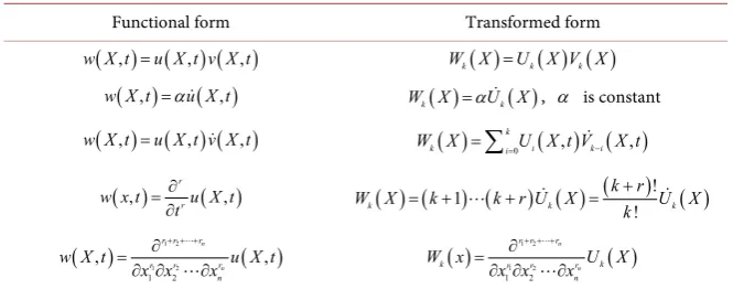
Table 1. Reduced differential transformation.

Functional form Transformed form

( ,) ( ,) ( , )

w X t =u X t v X t W X_k_{( )}=U X V X_k_{( ) ( )}_k

(

,

)

(

,

)

w X t =αu X t W Xk( )=αU Xk( ), α is constant

(

,

) (

,

) (

,

)

w X t =u X t v X t

( )

0

(

,

) (

,

)

k

k i i k i

W X =

∑

=U X t V− X t

( ), rr ( , )

w x t u X t

t ∂ = ∂ ( ) ( ) ( ) ( ) ( ) ( ) ! 1 !

k k k

k r W X k k r U X U X

k + = + _ +  = 

( ) 1 2 ( )

1 2

, r r rr rn r_n ,

n

w X t u X t x x x

+ + + ∂ = ∂ ∂ ∂   ( ) ( ) 1 2 1 2 1 2 n n

r r r

k r r r k

n

W x U X

x x x

+ + + ∂ = ∂ ∂ ∂  

In order to apply this method with KRLNS equations to find approximate analytical solutions for INS equations, we suppose that X =

( )

x y, _, u=

( )

u v, and Uk =

(

U Vk, k

)

, where u X t

(

,

)

and v X t

(

,

)

are the fluid velocity

components in the x and y directions, and U Xk

( )

, V Xk

( )

and G Xk

( )

are

t-dimensional spectrum functions of u X t

(

,

)

, v X t

(

,

)

and g X t

( )

, respectively. Then, we have

(

)

( )

(

)

(

( )

)

(

( )

)

1 1 1 2 , k

k k k k _x k _xx k _yy

k U X

A B C G X U X U X

Re + +   = −_ + + + − + _  

(

)

( )

(

)

(

( )

)

(

( )

)

1 1 1 2 , k

k k k k _y k _xx k _yy

k V X

D E F G X V X V X

Re + +   = −_ + + + − + _  

(

)

( )

(

( )

)

(

( )

)

(

( )

)

(

( )

)

1 2 1

1 1 _,

k

k _x k _y k _xx k _yy

k G X

U X V X G X G X

Re Ma + +     = −_ + − + _   (2.4) such that

( )

(

( )

)

( )

(

( )

)

0 , 0 ,

k k

k i k i _x k i k i _x

i i

A U X U − X B V X V− X

= =

=

∑

=

∑

( )

(

( )

)

( )

(

( )

)

0 , 0 ,

k k

k i k i _y k i k i _x

i i

C V X U − X D U X V− X

= =

=

∑

=

∑

( )

(

( )

)

( )

(

( )

)

0 , 0 ,

k k

k i k i _y k i k i _y

i i

E U X U − X F V X V− X

= =

=

∑

=

∑

where k=0,1,2,3,, U X0

( ) (

=u X,0

)

, V X0

( ) (

=v X,0

)

and

( )

(

)

0 ,0

G X =g X _{. Then the exact solution is obtained as follows:}

(

,

)

lim_n n

(

, ,

)

u X τ u X τ

→∞

=

(

,

)

lim_n n

(

, ,

)

v X τ v X τ

→∞

=

(

,

)

lim_n n

(

, ,

)

g X τ g X τ

→∞

(6)

(

)

( )

(

)

( )

(

)

( )

0 0 0

, n k, , n k, , n k.

n k n k n k

k k k

u X τ U X τ v X τ V X τ g X τ G X τ

= = =

=

∑

=

∑

=

∑

This approach is referred to by (KRDTM) in this paper.

3. Perturbation-Iteration Algorithm (PIA)

Perturbation methods are important analytical methods which have been used to construct approximate analytical solutions of algebraic equations, differential equations, and integro-differential equations. The main limitation of using the perturbation methods is to install a small auxiliary parameter in the equation. For this reason, the solutions of these methods are restricted by validity range of physical parameters, so many of perturbation techniques have been suggested by several authors. PIA is one of the techniques which was proposed by Pakdemirli and Boyac in [28], and used a combination of perturbation expansions and Tay-lor series expansions to construct an iteration scheme for using to generate root finding algorithms. It is applied by many authors to get the approximate analyt-ical solution for differential equations. In [29], PIA was applied to obtain the so-lution of Bratu-type equations. In [30], PIA was utilized to find the solution first order differential equations. This algorithm was tested on three nonlinear heat equations in [31]. Moreover, PIA was generalized to an arbitrary number of first-order coupled equations in [32]. It was applied to Fredholm and Volterra integral equations in [33]. Also, in [34], PIA was proposed for solving the Riccati differential equation. It was developed in [35] to obtain the solutions of Lotka-Volterra differential equations. In [36], some types of fractional differen-tial equation systems were solved by using this method. PIA with Laplace trans-form method was combined in [37] to solve Newell-Whitehead-Segel equations. In [38], PIA is used for solving the fractional Zakharov-Kuznetsov equation and compared with the residual power series method. By reviewing the previous li-terature, we have not found any research that has used this method to find a so-lution to the two-dimensional lid-driven cavity flow problem and which is an important reason to use this method to solve this problem.

In general, PIA is obtained by taking different numbers of terms in the per-turbation expansions and different order of correction terms in the Taylor series expansions. Therefore, the perturbation-iteration algorithm is called PIA(m,n) where the m is the number of the correction terms in the perturbation expansion and n is the highest order derivative term in the Taylor series such that m should always be less than or equal to n.

To obtain approximate analytical solutions for two-dimensions Navier-Stokes equations, PIA (1, 1) will be applied to KRLNS equations and which will be re-ferred to this article by (KPIA). Firstly, we write Equation (1.5) as follows:

(

)

(

)

1 , , , , , , , , ,

1

2 ,

t x y x x xx yy

t x x y x xx yy

F u v u u u v g u u

u uu vv vu g u u

Re

 

= + _ + + + − + _

 



(7)

(

)

(

)

2 , , , , , , , , ,

1

2 ,

t y x y y xx yy

t x y y y xx yy

F u v v u v v g v v

v uv uu vv g v v

Re   = + _ + + + − + _    

(

)

( )

(

)

(

)

3 2 , , , , ,

1 1 _,

t x y xx yy

F g u v g g

g u v g g

Re Ma     = + + − +     

 (3.1)

where  is a small perturbation parameter. Secondly, we define the following perturbation expansions with only one correction term:

( )

1 ,

n n c n

u+ =u + u

( )

1 ,

n n c n

v+ =v + v

( )

1 ,

n n c n

g + =g + g (3.2) where n represents the n_th iteration and uc, vc and gc are the correction

terms in the perturbation expansion. Thirdly, by replacing (3.2) into (3.1) and writing in the Taylor series expansion for first order derivative terms about

0

=

 , yields

( ) ( ) ( ) ( ) ( ) ( ) ( )

(

)

( )

₍ ₎

(

( )

)

( )

(

( )

)

( )

(

( )

)

( )

(

( )

)

( )

(

( )

)

( )

(

( )

)

( )

(

( )

)

1 1 1

1

1 1 1 1

1 1 1

, , , , , , , , ,0

0,

n n n t

n x n y n x

n x n xx n yy

n n n _t n _x n _y n _x n _x n _xx n _yy

u c n v c n u c n t

c c c

u n _x u n _y v n _x

c c c

g n _x u n _xx u n _yy

F u v u u u v g u u

F F u F v F u

F u F u F v

F g F u F u

+ + + + + + + + +  + _ + + + + + +  + + + _=  

( ) ( ) ( ) ( ) ( ) ( ) ( )

(

)

( )

₍ ₎

(

( )

)

( )

(

( )

)

( )

(

( )

)

( )

(

( )

)

( )

(

( )

)

( )

(

( )

)

( )

(

( )

)

1 1 1

2

2 2 2 2

2 2 2

, , , , , , , , ,0

0,

n n n t

n y n x n y

n y n xx n yy

n n n t n y n x n y n y n xx n yy

u c n v c n v c n t

c c c

u n y v n x v n y

c c c

g n y v n xx v n yy

F u v v u v v g v v

F F u F v F v

F u F v F v

F g F v F v

+ + + + + + + + +  + _ + + + + + +  + + + _=  

( ) ( ) ( ) ( ) ( )

(

)

( )

(

( )

)

( )

(

( )

)

( )

(

( )

)

( )

(

( )

)

( )

(

( )

)

1 1 1

1 1

3

3 3 3 3

3 3

, , , , ,0

0.

n t n x n y

n xx n yy

n t n x n y n xx n yy

c c c

g n _t u n _x v n _y

c c

g n xx g n yy

F g u v g g

F F g F u F v

F g F g

+ + + + +  + _ + + +  + + _= 

 (3.3)

All derivatives in Equation (3.3) are evaluated at =0 such that

( ) ( ) ( ) ( ) ( ) ( ) ( )

(

)

( )

1 n, ,n n t, n x, n y, n x, n x, n xx, n yy,0 n t,

F u v u u u v g u u = u

( ) ( ) ( ) ( ) ( ) ( ) ( )

(

)

( )

2 n, ,n n t, n y, n x, n y, n y, n xx, n yy,0 n t,

F u v v u v v g v v = v

( ) ( ) ( ) ( ) ( )

(

)

( )

3 n t, n x, n y, n xx, n yy,0 n t,

F g u v g g = g

( 1) ( 1) ( 1)

1un t 1vn t 3gn t 1,

(8)

( ) ( ) ( ) ( ) ( )

1 1 1 1 1 1 1

1un 1vn 1un x 1un y 1vn x 1un xx 1un yy 0,

F ₊ =F ₊ =F ₊ =F ₊ =F ₊ =F ₊ =F ₊ =

( ) ( ) ( ) ( ) ( )

1 1 1 1 1 1 1

2un 2vn 2vn x 2vn y 2un y 2vn xx 2vn yy 0,

F ₊ =F ₊ =F ₊ =F ₊ =F ₊ =F ₊ =F ₊ =

( 1) ( 1) ( 1) ( 1) ( 1) ( 1)

1gn x 2gn y 3un x 3vn y 3gn xx 3gn yy 0,

F ₊ =F ₊ =F ₊ =F ₊ =F ₊ =F ₊ =

( )

( ) ( )

(

( ) ( )

)

1 2 n n x n n x n n y n x 1 n xx n yy ,

F u u v v v u g u u

Re

 

=_ + + + − + _

 



( )

( ) ( )

(

( ) ( )

)

2 n n x n n y 2 n n y n y 1 n xx n yy ,

F u v u u v v g v v

Re

 

=_ + + + − + _

 



( )

(

( ) ( )

)

(

( ) ( )

)

3 2

1 1 _.

n _x n _y n _xx n _yy

F u v g g

Re Ma

 

 

= + − +

 

 



Finally, by substituting the above derivative in the formulas (3.3) and setting

1

=

 we obtain the following iteration equation formulas:

( )

(

uc n

)

t

( )

un t 2u un

( )

n x v vn

( )

n x v un

( ) ( )

n y gn x Re1

(

( ) ( )

un xx un yy

)

,

 

= −_ + + + − + _

 

( )

(

vc n

)

t

( )

vn t u vn

( )

n x u un

( )

n y 2v vn

( ) ( )

n y gn y _Re1

(

( ) ( )

vn xx vn yy

)

,

 

= −_ + + + − + _

 

( )

(

)

( )

2

(

( ) ( )

)

(

( ) ( )

)

1 1 _.

c n _t n t n x n y n xx n yy

g g u v g g

Re Ma

 

 

= −_ + − + _

  (3.4)

The calculations start with initial condition u x y

(

, ,0

)

, v x y

(

, ,0

)

and

(

, ,0

)

g x y where these values are used as estimate values for

( )

uc ₀,

( )

vc 0 and

( )

gc ₀ in Equation (3.4), and then substitute the results of Equation (3.4) into

Equation (3.2) to obtain u1, v1 and g1 which are the solutions at the first

iteration. So we can get

(

n+1

)

_{iteration solutions by repeating this process and} using the previous solution n as an initial guess.

4. Analysis of Convergence

We now study the convergence analysis of the approximate analytical solutions which are computed from the application KRDTM and KPIA.

Let us consider the Hilbert space _{H L a b}₌ 2

(

( )

_, 2_×

[ ]

_0,_T

)

_{as defined by}

( )_, 2 [ ]_0, 2

(

)

: with _{a b} _T , d d ,

u H →_

_∫

_× u X t X t< ∞ and the norm

( )2 [ ]

(

)

2 2

, 0, , d d ,

a b T

u =

_∫

_× u X t X t where X =

( )

x y, _{. Defined as}

(

u v g H, , :

)

3 3with _{( )}_{a b}_, 2_×_{[ ]}_0,_T

(

u X t v X t2

(

,

)

2

(

,

)

g X t2

(

, d d < ,

)

X t

= →

_∫

+ + ∞

u

such that u2 = u 2+ v2+ g 2.

We consider the KRINS equation in the following form

(

)

(

X,τ

)

=

(

X,τ

)

+

(

X,τ

)

,

(9)

DOI: 10.4236/jamp.2018.612211 2526 Journal of Applied Mathematics and Physics which is equivalent to the following formula

(

X,τ

)

=

(

k

(

X,τ

)

,

u u (4.2) where  is the linear partial derivative with respect to τ,  is a nonlinear operator,  is a linear operator, and  is a general nonlinear operator involving both linear and nonlinear terms.

Case 1: According to KRDTM, formula (4.1) can be written in the following form

(

k+1

)

Uk+1

( )

X =

(

Uk

( )

X

)

+

(

Uk

( )

X

)

, and the solutions

(

)

( )

0 0

, k ,

k k

X τ ∞ X τ ∞

= =

=

∑

=

∑



u U (4.3)

where k =

(

  1k, 2k, 3k

)

. It is noted that the solutions by KRDTM is

equivalent to determining the sequence

( )

0= 0 X =0,

S U

( )

1= 0 X + 1 X

τ

= 0+ 1,

S U U

( )

2

2 = 0 X + 1 X

τ

+ 2 X

τ

=  0+ 1+ 2,

S U U U



( )

0 0 .

n n

k

n k k

k X k

τ

= =

=

∑

=

∑



S U

Case 2: To study the convergence of KPIA, we write the approximate solutions in different form. To do this, we define

(

)

(

) (

)

(

)

0 = 10, 20, 30 = u X,0 ,v X,0 ,g X,0 = X,0 ,

    u

( ) ( ) ( )

(

)

( ) (

) ( ) (

)

(

)

( ) (

)

1 1 1, 2 1, 3 1

, , , , , , ,

n n n n

c n c n c n c n

u X τ v X τ g X τ X τ

+ = + + +

= =

   

u

0=0= 0,

u S

( )

1= 0+ c 0= 0+ 1= 1,

u u u S

( )

2= 1+ c 1=  0+ +1 2= 2,

u u u S

( )

3= 2+ c 2=   0+ +1 2+ 3= 3,

u u u S



( )

1 1 0 1 2 3

0 .

n

n n c n n k n

k

− −

=

= + ≡ + + + + + =

∑

=

u u  u        S

So the solutions, which are resulted from KPIA have the form

(

)

( )

0 0

, k .

k k

X τ ∞ X τ ∞

= =

=

∑

=

∑



u U (4.4)

(10)

DOI: 10.4236/jamp.2018.612211 2527 Journal of Applied Mathematics and Physics The sufficient condition for convergence of the series solution

{ }

n ₀

∞

S is given in the following theorems.

Theorem 4.1. The series solution

{

n

(

R S Tn, ,n n

)

}

₀

∞

=

S converges whenever there is γ such that 0< <

γ

1, γ γ= +1 γ2+γ3 and i k( +1) 

γ

i ik .

Proof: Firstly, we show that

{

n

(

R S Tn, ,n n

)

}

₀

∞

=

S is a Cauchy sequence in the Hilbert space _H3_{. For this reason, we suppose that}

( ) 2 ( ) 1

1 1 1 1 1 1 1 1 1n 10 ,

n n n n n

R R

γ

+

+ − =  +     −   

( ) 2 ( ) 1

1 2 1 2 2 2 2 1 2n 20 ,

n n n n n

S S

γ

+

+ − =  +     −   

( ) 2 ( ) 1

1 3 1 3 3 3 3 1 3n 30 .

n n n n n

T T

γ

+

+ − =  +     −   

Then, by using the triangle inequality, we find that

(

) (

)

1 1 2 1

, , , , , ,

n m n n n m m m n m n m n m

n m n m n m

n n n n m m

R S T R S T R R S S T T

R R S S T T

R R R R R R

S S S S S S

T T T T T T

− − − + − − − + − − − + − = − = − − − − + − + − − + − + + − + − + − + + − + − + − + + −      S S

(

)

(

)

(

)

(

)

(

)

(

)

(

)

1 1 1 1

1 1 1 10 2 2 2 20

1 1

3 3 3 30

1 1

10 20 30

1 1 2

10 20 30

1 0

1

, 1

n n m n n m

n n m

m n m n m

m

γ γ γ γ γ γ

γ γ γ

γ γ − + − + − + − + + − − − − + + + + + + + + + + + + + + + + + = + + + + + −                  

since 0 < ∞ and 0< <

γ

1, we then have limn m, →∞ S Sn− m =0. Thus, we

conclude that

{ }

n ₀

∞

S is a Cauchy sequence in the Hilbert space H3_{, thus, the}

series solution

{ }

n ₀

∞

S converges to some

{ }

_S _∈_H3_.

Theorem 4.2.Let  =

(

  1, ,2 3

)

be a nonlinear operator satisfies Lipschitz

condition from a Hilbert space H3_into_H3_and _u

(

_X_,

_τ

)

_{be the exact solution of}

INS equations. If the series solution

{ }

n ₀

∞

S converges, then it is converged to

(

X,

τ

)

u .

Proof: Let u1

(

X, ,

τ

) (

u2 X,

τ

)

, then we have

( )

(

)

(

( )

)

( )

(

)

( )

(

)

1 2

1 1 2 1 3 1 1 2 2 2 3 2

1 1 1 2 2 1 2 2 3 1 3 2

1 1 2 2 1 2 3 1 2

1 2 3 1 2 1 2

, , , ,

, ,

.

α α α

α α α α

− = − = − − − − + − + − − + − + − = + + − = −                       u u

u u u u u u

u u u u u u

u u u u

Therefore, from the Banach fixed-point theorem, there is a unique solution of the problem (4.1). Now we have to prove that

{ }

n ₀

∞

(11)

(

)

(

)

( )

0 0

1 0

, , lim

lim lim lim .

n

k _n k

k k

n

k n n

n _k n n

X τ X τ ∞

→∞

= =

+

→∞ ₌ →∞ →∞

   

= = _ _= _ _

   

 

= _ _= = =

 

∑

    

  

u u

S S S

Definition 4.1. For i=1,2,3_and k∈

{ }

0 , we define

( 1)

, 0,

0, 0.

i k

ik ik _ik

ik

γ

+



 _≠

 =  

= 



 



then we can say that the series approximate solutions

{ }

n ₀

∞

S converges to the exact solution u

( )

X t, when γk =γ1k+γ2k+γ3k and 0<γk <1 for all

{ }

0

k∈ .

5. The Two-Dimensional Lid-Driven Cavity Flow

In this work we presented the recirculation viscous flow problem in a square cavity, that is called Burggraf Flow [10] [39] [40] [41] [42] [43], and has exact solutions in a steady state as a form

( )

( ) ( )

( )

( ) ( )

( )

(

( ) ( )

)

( ) ( ) ( )

(

( )

)

2

)

1

, 8 ,

8 ,

64 ,

u x y f x g y v x y f x g y

p x y F x g x f x g x

Re

F x g y g y g y

′ =

′ = −

′′′ ′ ′

= +

′′ ′

+ −

(5.1)

where

( )

4 ₂ 3 2_,

( )

4 2_,

f x =x − x +x g x =y −y

( )

d , 1

( )

( ) ( )

d ,

F x =

_∫

f x x F x =

_∫

f x f x x′ such that the stream function ψ _{and vorticity}ω are defined as

( ) ( )

8f x g y , such that y u, & x v,

ψ

=

ψ

=

ψ

= −

( ) ( )

(

)

8 .

x y

v u f x g y f x g y

ω= − = − ′′ + ′′

The boundary conditions for the velocities u and v in this problem are of Dirichlet type, which are equal to zero everywhere except along the top surface where

(

_,1,

)

₁₆

(

4 ₂ 3 2

)

_.

u x t = x − x +x

To obtain the approximate analytical solutions of the unsteady lid-driven cavity flow problem, we consider the analytical solutions to this problem, which are given in (5.1) as initial conditions for u, v and p.

Then, by applying KRDTM with the initial conditions of this problem, we obtained the iterative solutions like the form (2.5), such that

( )

1 , 0,

(12)

( )

(

)

( )

(

)

(

)

(

) (

)

(

) (

)

(

)

(

)

(

)

2 2 2 8

2 2 2

2

4 2 4 2 7 4

2 6 6 4 2 5

6 4 2 4 8 6 4

2 3 6 4 2 2 2

192 256

, 12 2 12 1 3 2 9 6 1

5

30 1 4 531 102 1 14 531

156 10 2520 7344 2244 215

25 252 9 9 5 5 72 932 660

264 5 5 108 138 201 111

U x y x y x y x y x

Re Re

y y y y x y

y x y y y x

y y y x y y y

y x y y y x y

 = − + − + + _ − − − − + − + − − + + + − + − − + + + + − + + − + − +

(

)

(

)

(

)

(

) (

)

(

)

(

)

(

)

6 4 2 2

2

2 6 4 2 4

2

2 4 2 6 4 2 7

8 6 4 2 6

8 6 4 2 5

5 48 62 19 11

1024 1 6 2 5 4 1

44 2 1 1 36 18 8 1 4

2 90 236 105 37 3

2 270 456 189 55 2

y y y xy

x x y y y y y

y y y x y y y x x

y y y y x

 + − + + _  − − _ − + − − − − + − + − − − − + − + + − + − +

(

)

(

)

(

)

10 8 6 4 2 4

8 6 4 2 3 2

8 6 4 2 2 2

144 954 1172 429 93 1

8 36 126 124 39 5

232 634 544 149 7 ,

y y y y y x

y y y y x y

+ − + − + − − − + − +  + − + − + _ 

( )

(

)

(

)

(

)

(

)

(

)

(

)

(

)

(

)

(

)

4 2 4 5 2 3

1

2 2 4 2

2

2 4 2 3

6 4 2 2 4 2 2

32 2

, 3 2 12 1

5

6 6 1 2 3 3 1

128 1 6 2 1 2

8 18 6 1 2 2 3 1 2 1 ,

V x y y y x x y x

Re

y x y y x

x x y y x x

y y y x y y x y

   = _{ }_ − + − _− −    + − − + − _  + − _ − + −  − − + − + − + − _

( )

(

)

(

)

(

)

(

)

(

)

2 3 2

2 2

7 6 5 4 3 2 5

8 7 6 5 4 3 2 3

2 5 4 3 2

192

, 12 2 1 10 15 2

256 10 15 108 324 334 128 10 1 5

864 3456 4652 1860 710 480 30 5

1 132 396 130 400 315 45

V x y x y x x x

Re

y x x x x x y

Re

x x x x x x x y

x x y x x x x x

= − − + − + +  + _ + − + − + − + − + − − + + +  − − − + + − + _

(

) (

)

(

)

(

)

(

)(

)

(

)

(

)

3

3 2 10

4 3 2 8

2 2 6

2

4 3 2 4 2 2

2048 1 2 1 4 16 16 9

2 15 30 81 66 37

2 18 18 23 1

7 14 21 14 8 1 ,

x x x x x y

x x x x y

x x x x y x x y

 − − − _ − + − − + − + + − + − +  − − + − + + − _ 

( )

(

2 2

)

(

)

1 2

192

, 4 2 4 1 2 1

G x y x y x x y

Re

(13)

(

)

(

)

(

)

(

)

4 2 7

6 4 2 6

6 4 2 5

128 3 50 18 1 4

6 84 68 32 3

12 126 73 15 1

y y x x

Re

y y y x

 + _− − + − − + − + + − + +

(

)

(

)

(

)

(

)

(

)

8 6 4 2 4

6 4 2 3 2

6 4 2 2 2

2 4 2

120 1388 1320 372 3

16 15 16 30 12

2 78 98 21 15

2 1 18 1 ,

y y y y x

y y y x y

y y x

− + − + + + + − + − − + + + − −

( )

(

)

( )

(

)

(

)

(

)

(

)

(

)

(

)

(

)

2 7

2 3 2

4 2 6 4 2 5

6 4 2 4

6 4 2 3

8 6 4 2 2

3456 256

, 2 1 9 50 3 4

6 980 78 9 18 980 272 12

3 1820 4490 1800 107

12 910 205 45 13

6 60 1058 905 207 4

G x y y x y x x

Re Re

y y x y y x

y y y x

y y y y x

 = − + _− − − − + − + − + − + − + + − − + − + − + +

(

)

( )

(

)

(

)

( )

(

)

(

)

(

)

(

)

(

)

(

)

6 4 2 2 2 4

6 8 2 2

2

2 4 2 3

2

6 4 2 2

6 4 2 4 2 2

6 60 148 210 66 21 9

96

70 78 4 2 4 1 2 1

64 ₁ ₃₀ ₆ ₁ ₂

56 90 18 1

2 28 30 6 2 14 15 3 ,

y y y y x y y

y y x y x y x

Ma Re

x x y y x x

Ma

y y y x

y y y x y y y

+ + − + − +  + − _+ + − − −  − − _ − + − − − + −  + − + − − + _ 

To make a decision on the convergence of the KRDTM, we computed γk as:

(

)

(

)

1 10 0 , 0, ,

U x y U x y

τ

γ = =

( )

(

2

)

1 20

0

714 3227504 12514788 1994117697

,

, 14586

,

Re Re

V x y

Re V x y

τ _τ

γ = = − +

( )

(

)

( )

2 1 30 2 0

60 49405942 1467358893

,

, 1253680 21900879 292485765

Re G x y

Re

G x y Re Re

τ _τ

γ = = +

− +

( )

2 2 11 1 , 0, ,

U x y U x y

τ

γ

τ

= =

(

)

(

)

(

( )

2 2 4 21 1 3 2 , 16422 4861754265600 , 2305887904320 15827448430362608

V x y

Re V x y

(14)

)

( )

(

)

0.5

0.5 2

25967180162523600 3689889931130027625

260015 3227504 12514788 1994117697 ,

Re

Re Re Re



− + _

 

÷_ − + _

 

( )

(

)

( )

(

( )

(

)

( ) ( )

( )

(

)

( )

(

)

( )

2 2

31 1

2 4

2 2 2

0.5

2 4

0.5

2 2

, ,

3 2007409369056 14901358071600

1477832512 165570645240

20792594 4402076679

6 49405942 1467358893 ,

G x y G x y

Re Ma

Re Re Ma

Re Re

Re Re Ma

τ γ

τ

=



= _ +

+ −



+ + _

 

÷_ + _

 



such that γ0=γ10+γ20+γ γ30, 1=γ11+γ21+γ31,. For example, if Ma=0.1,

0.1

t= _{, and}Re=1_{such that}τ =Ma t× _{, for all}_x_and_y_{in domain}

[ ]

0,12, then

0 0.9991283888 1, 1 0.7958329986 1, ,

γ = < γ = < _

if Ma=0.1, t=0.01, and Re=10 then

0 0.0129736262 1, 1 0.2936820858 1,

γ = < γ = < _

Thus, the iterative solutions (3.2) for this problem, which are obtained by using KPIA, have the following form

(

)

2

(

2

)

(

)

2

1 , , 16 2 1 1 ,

u x yτ = x y y − x−

(

)

(

)

(

)

( )

(

)

(

)

(

)

(

)

(

) (

)

(

)

(

)

2

2 2 2 2

2 2

2 8 4 2 7

4 2 6 6 4

2 5 6 4 2 4

8 6 4 2 3

192

, , 16 2 1 1 12 12 2 1

256 3 6 1 2 9 4 531 102 1

5

14 531 156 10 2520 7344

2244 215 25 252 9 9 5

5 72 932 660 264 5

y

u x y x y y x x x y

Re

y x x y y x

Re

y y x y y

y x y y y x

y y y y x

τ = − − + − − + +



+ − − + − +

− − + + +

− + − − + + + + − + +

(

)

(

)

(

)

(

)

(

)

(

)

(

)

(

)

6 4 2 2 2

2

6 4 2 2 4 2

2

2 6 4 2 7

8 6 4 2 6

8 6 4 2 5

5 108 138 201 111

5 48 62 19 11 30 1

1024 1 36 18 8 1 4

2 90 236 105 37 3

2 270 456 189 55 2

y y y x y

y y y xy y y

x x y y y y x x

y y y y x

− + − +

+ − + + − −

− − − + − −

− − + − + + − + − +

(

)

(

)

10 8 6 4 2 4

8 6 4 2 3 2

144 954 1172 429 93 1

4 72 252 248 78 10

y y y y y x

y y y y x y

(15)

(

)

(

) (

)

(

)

(

)

(

)

(

)

(

8 6 4 2 2 2

2

2 4 2 6 4 2 4 2

3 2 2 2

232 634 544 149 7

44 2 1 1 6 2 5 4 1

1

16384 3 2 3 12 1 6 6 1

y y y y x y

y y y x y y y y

x x y x y x

Re τ + − + − +  − − − + − + − _  − _− − + − − − 

)

(

)

(

)

(

)

(

)

(

) (

)

(

)

(

)

(

)

(

4 2 4 2 6

6 4 2 5 6 4 2 4

6 4 2 3 4 2 2

4 2 3

3 3 1 8 6 2 1 2 7

3 4 24 8 3 5 6 15 5 1

28 48 16 1 2 3 1 6 1

1 _{3 2} ₅ _{10 12} ₁

120

y y y y y x x

y y y x y y y x

y y y x y y x xy

x x y x

Re + + − + − + − − − + − + − + − − − + − + − + −  × −_ − + − 

(

)

(

)

(

)

(

)

(

)

(

)

(

) (

)

(

)

(

)

2 2 4 2 2 2

4 2 7 6 4 2 6

6 4 2 5 6 4 2 4

4 2 2 2 3

30 6 1 10 3 3 1 15 1

6 2 1 4 2 4 24 8 3

6

4 6 15 5 1 28 48 16 1

2 2 3 1 4 1 ,

y x y y x y y

y _y _y _x _x _y _y _y _x

y y y x y y y x

y y x x y τ

− − + + − − − + − + − − − + − + − + − − − + −  + − + − _ 

(

)

(

)(

)

(

)

(

)

(

)

(

)

(

)

(

)

(

)

(

)

(

)

5

3 2 4 2 4 2 4

1

2 3 2 2 4 2

2

2 4 2 3

6 4 2 2 4 2 2

32 2

, , 16 2 3 3

5

2 12 1 6 6 1 2 3 3 1

128 1 6 2 1 2

8 18 6 1 2 2 3 1 2 1 ,

x

v x y x x x y y y y x

Re

y x y x y y x

x x y y y x x

y y y x y y y x

τ τ     = − − + − +  _ − + −        − − + − − + − _  + − − + −  − − + − + − + − _ 

(

)

(

)(

)

(

)

(

)

(

)

(

)

(

)

(

)

(

)

(

)

(

)

(

)

(

)

(

)

_{( )}

(

)

3 2 4 2 4 2 7

2

6 4 2 6 6 4 2 5

6 4 2 4 4 2 2 2

4 2 3 2 2

4 2 2 2

2

, , 16 2 3 128 6 2 1 4

2 4 24 8 3 2 12 30 10 2

28 48 16 1 2 2 3 1 4 1

1 _{3 2} ₅ _{10 12} ₁ _{30 6} ₁

20

192

10 3 3 1 15 1 2 1

v x y x x x y y y y y x x

y y y x y y y x

y y y x y y x x y

x x y x y x

Re

y y x y y x

Re τ τ  = − − + − + _ − + − − − + − + − + − − − + − + − + − − − + − − −   + + − − − _ + − − 

(

)

(

)

(

)

(

)

(

)

(

)

(

)

(

)

(

)

(

)

(

) (

)

(

)

2 2 2 7

4 2 6 4 2 5

4 2 4 4 2 3

4 2 2 4 2 2

3 2

2 3 2 2

256

5 5 12 2 12 72 11 4

5

2 810 2326 263 30 162 62 9

5 1002 142 143 120 16 4 3

15 10 2 3 5 2 3 1

512 1 1 2 1 1

y

x x y y x x

Re

y y x y y x

y y x y y y

y x x x y x x

× − + − + − −

+ + − − + +

+ − + − − +

+ + + + − +

(16)

(

)

(

)(

)

(

)(

)

(

)

(

)

(

)

(

) (

)

(

)

(

)

(

)

2 6 2 2 4

2 2 2 2 4

2 7 6 4 2 6

6 4 2 5 6 4 2 4

4 2 2 2 4

4 16 16 9 2 15 15 19 1

512

2 3 3 4 1 20 6

15

2 1 4 2 4 24 8 3

2 12 30 10 2 28 48 16 1

1

2 2 3 1 4 1 3 2 5

x x y x x x x y

x x x x y y y

y x x y y y x

y y y x y y y x

y y x x y x x

Re τ − − + + − + − +   − − + − + _ + −_  − + − − − + − + − + − − − + − + − + − − −

(

)

(

)

(

)

(

)

(

)

(

2 3 2 2 4 2

2 2 4 2 7

6 4 2 6 6 4

10 12 1 30(6 1) 10(3 3 1)

15 1 2 30 6 1 4

4 28 120 24 3 8 42 75

y x y x y y x

y y y y x x

y y y x y y

+ − − − + + − − − × − + − − − + − + −

)

(

)

(

)

(

)

(

)

(

)

(

)

2 5 6 4 2 4

6 4 2 3 6 4 2 2

2 2 2 3

15 1 2 196 240 48 1

16 14 15 3 4 14 15 3

3 4 2 3 2 2 1 2 1 ,

y x y y y x

y y y x y y y x

y _x _x _y _x _y

Re

τ

+ − − − + − + − + − − +   − − + + − _{+ }  

(

)

(

)

(

)

(

)

(

)

(

)

(

)

(

)

(

)

( )

(

)

(

)

2

2 2 2

1

2 2 2 4 2 3

2

6 4 2 2 2 2

2 2

2

32 6

, , 4 3 2 1 3 1

5

64 1 10 9 3 2

8 6 3 2 1 4 1

192 2 1 4 2 4 1

xy x

g x y y x x y x

Re

x x y y y x x

y y y x y y x

x x y x y

Re

τ =  − +  − − − 

      − − _ − + −  + − − + − − _{− }  − − + − − 

(

)

(

)

(

)

(

)

(

)

(

)

(

)

(

)

(

)

4 2 7 6 4

2 6 6 4 2 5

8 6 4 2 4

6 4 2 3 2 6 4

2

2 2 2 4 2

128 3 50 18 1 4 6 84 68

32 3 6 252 146 30 2

120 1388 1320 372 3

16 15 16 30 12 2 78 98

21 15 2 18 1 1 ,

y y x x y y

Re

y x y y y x

y y y y x

y y y x y y y

y x y x y y τ

− − + − + + − + − − + + + + − + + − + − + + −  + + − − − 

(

)

(

)

(

)

(

)

(

)

(

)

(

)

(

)

(

)

(

)

(

)

(

)

(

)

(

)

(

)

(

)

2

2 2 4 2 3

2

6 4 2 2 2 2

4 3 2 2

2 2 4

2

2 7 6 4 2 6

, , 64 1 10 9 3 2

8 6 3 2 1 4 1

32 3 2 5 20 5 2 1 3 1

5

192 128

[ 2 1 4 4 2 1 3 50

( )

18 1 4 6 84 68 32 3

g x y x x y y y x x

y y y x y x y

y _x _x _{x y} _y _x _x

Re

y x x x y y

Re Re

y x x y y y x

τ = − − − + −

+ − − + − − −

+ − + − − −

+ − − + − − − + − + + − +

(

6 4 2

) (

5 8 6

12 126y 73y 15y 1 x 120y 1388y