An optimization approach between service level and inventory via simulation : an example from the semiconductor industry

(1)

1

Faculty of Behavioural, Management and Social sciences

Department of Industrial Engineering and

Business Information Systems

An optimization approach

between service level and

inventory via simulation:

an example from the

semiconductor industry

S.E. Lingelbach M.Sc. Thesis Munich, May 2017

(2)

(3)

Management summary

Company & Motivation

This graduation project is conducted as part of the Industrial Engineering and Management master program in cooperation with Infineon Technologies AG. Infineon is a German semi-conductor manufacturer producing chips, sensors, and microcontrollers. To stay competitive and satisfy customer demand quickly Infineon places inventory at various stock points within their supply chain. However, the more products are stored, the higher the costs due to the binding capital effect of stock. Thus, Infineon has to balance the trade off between high stocks (characterized by a highα-service level) and high costs when examining its supply chain plan-ning processes. In this thesis, we concentrate on the planplan-ning process of two products: chips for contactbased and contactless payment of the Chip Card & Security (CCS) department. The relevance lies in their high production volume and revenue share of more than 25% of CCS‘s total revenues.

Research objective

The graduation project aims to solve the below stated research objective:

Improve the supply chain planning process according to the service level and respective costs at CCS for two particular products considering the stocking strategies as well as the approach of quantifying the amount of wafers to be released to production.

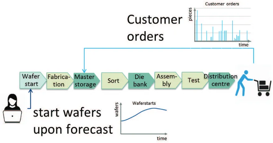
The stocking strategy concerns the decision where to place inventory and which amount to be stored. The production release approach examines the question how to quantify the amount of wafers (release quantity) to be started in production in advance. Usually, the pro-duction of wafers, which are thin slices of semiconductor material and serve as basis for many products, is started on forecast due to long processing times. This enables faster response to customer demand. A clever chosen approach of estimating the needed quantity helps cutting costs as stock levels can be reduced at the same α-service level.

Methodology

(4)

the total area between the cumulative distributions of the two demand series. The iterations are stopped when the total area is < 10% of the area below the cumulative distribution of the observed demand. To check the consistency of the chosen demand series we further apply the Chi-Square test.

Analysis of current situation

Infineons supply chain has three stock points (up- to downstream): the master storage, die bank, and distribution centre. The amount of products stored at these stock points is determ-ined by the target reach. The target reach is defdeterm-ined as the safety stock in number of weeks. Currently, CCS has a target reach of 13 weeks at the master storage, and no stocks at the die bank nor the distribution centre since the customer order decoupling point (CODP) lies at the master storage and thus products become customer specific in the downstream man-ufacturing steps. Storing at the master storage employs the risk pooling effect. The stocks are managed periodically (per week). The production up to the master storage is done on forecast by using a four monthmoving average (MA)over the historical data. The remaining manufacturing steps are continued when a customer order arrives. The overall performance can be given by the α-service level. The α-service level becomes either 100% when all orders are satisfied by the on-hand inventory during period t, or it becomes 0% when demand is not satisfied completely from stock. Currently, the α-service level is 98%.

Conclusion

• Both new production release approaches: a simpleMA over five weeks as well as single exponential smoothing (SES) outperform the current approach that uses a simple four months MA since they allow faster reaction in production as fluctuations are not as smoothed out as with a large time horizon of four months.

• Applying either of these new approaches costs can be cut by 40% since the target reach can be reduced from 13 to five weeks while keeping an α-service level of 98%.

• Comparing the simpleMAover five weeks andSES, the moving average performs slightly better. In addition, as it is easy to understand and to apply, we recommend to use the simple MA with a five week time window. That is, reducing the current time window from 16 to five weeks.

• When keeping the current production release approach, the target reach at the master storage can be reduced from 13 to about eight weeks while having only a marginal drop by around 0.5% in the α-service level of currently 98%.

Recommendations

• Enhance the demand generation method of the simulation model such that it is able to create intermittent and autocorrelated demand which is currently not supported by the simulation model. Note, the products we are considering do not show autocorrelation nor are classified as intermittent, however there are autocorrelated and intermittent products at Infineon.

• In addition, implement machine capacity and idle costs as currently capacity is unlim-ited and costs are solely evaluate according to the WIP and stock levels. However, in reality capacity is restricted and idle costs play an important role as machines are very expensive.

(5)

(6)

(7)

Preface

I hereby proudly present you my master’s thesis. This marks the end of a wonderful, exciting, and instructive chapter of my life - my studies in Industrial Engineering at the University of Twente - but it also marks the beginning of a new chapter - starting my first real job at Infineon and eventually being a grown up. Staying at this point I want to thank a few people who guided me during this research and supported me throughout my studies.

First of all, I want to thank Frank Federmann, my company supervisor, for the enormous support he gave me. He patiently guided me through this research and always found time to discuss issues that came up, helped me with problems I struggled with, and provided me with valuable ideas. Also, I am very grateful for the support of the whole scenario & econometrics team and my initiation into their team. Not only the digestive walks after lunch refreshed my mind, but I also enjoyed our after work activities like go karting and ‘escaping the room’. I am sure this will continue.

My special thanks goes also to Ahmad Al Hanbali, my university supervisor, without whom I would not have ended up at Infineon as he provided me with the contact when I told him that I want to go to the southern part of Germany, closer to the Alps. He contributed to this research by giving very useful advice and detailed reviewed the thesis. Thanks also to Matthieu v.d. Heijden for providing me with feedback and remarks.

Last but not least I want to say ‘thank you’ from the bottom of my heart to my beloved family (my mum Jutta & her partner Werner, my brother Yannick, and my sister Lara), relatives, and friends (sorry for not mentioning you by name, but that list would be quite long) who paved my way throughout my studies and went along this sometimes easy and fun but also sometimes rough and steep path. Without my mum, Jutta, I would not be where I am now as she always found the right words to encourage and motivate me during my whole studies and research whenever I felt lost. Also, she took care of the financial resources that are necessary when enjoying the student life, thanks also to my grandparents, Helga and Walter, as well as my godparents, Heidi and Eckhard. In addition, I am so grateful to have my twinsister, Lara. We do not need many words or emojis to understand each other and I can always rely on her. Together, we spent our weekends in the library cheering up one another and supporting each other. Finally, even though our path partly split up, I want to thank Julian who supported my decision to do my master studies in the Netherlands and came along. He was never tired of cheering me up and motivating me to another triathlon training session.

I certainly could fill some more pages with friends who I would like to thank, so to every-one I did not mentievery-oned explicitly, but who I studied, did sport, lived, and worked with: ‘THANK YOU VERY MUCH’ !

(8)

(9)

Acronyms

ADI average inter-demand interval. 36

asp average selling price. 33

ASSY assembly. 33

ATV Automotive. 1,17

BE back end. 28,33

CCS Chip Card & Security. 1,8,15,52

CI confidence interval. 70

CODP customer order decoupling point. 61,62,64

CT cycle time. 14,15,28,33,Glossary: cycle time

CV coefficient of variation. 20

CV2 squared coefficient of variation. 36

DB die bank. 28

DC distribution centre. 14,28

DES discrete event simulation. 1

DMOP data mart order processing. 19

DR delivery reliability. 16,17

DTW dynamic time warping. 42

FAB fabrication. 13,33

FE front end. 28,33

FF freeze fence. 30,Glossary: freeze fence

(14)

Acronyms

IPC Industrial Power Control. 1

KPI key performance indicator. 16,32

MA moving average. 37,38

MAE mean absolute error. 39

MS master storage. 28

MSE mean squared error. 38

PMM Power Management & Multimarket. 2

POD proof of delivery. 16

RMSE root mean squared error. 39

SCOR Supply Chain Operations Reference Model. 11

SES single exponential smoothing. 38,62

SP sales product. 20,Glossary: sales product

TC total costs. 32–34

wacc weighted average cost of capital. 33,34

WIP work in process. 8,33

WS wafer start. 28

(15)

Glossary

basic type Basis product that receives customer specific information in the sort, thereby splitting up into a variety of sales products. 13,15

customer order Order by customers. They contain the required quantity and delivery date for the needed sales products, which is binding. 4

freeze fence The number of periods from now onwards into the future where demand does not get modified. That is, if the freeze fence is three weeks, we know the orders for sure that arrive in the following three weeks. 30

marketing forecast Forecast made by marketing. They use a four month moving average over the observed demand to determine the needed quantity for the two basic types. 4, 29

production release approach It is the approach of quantifying the amount of wafers to be released to production in advance. 3,61

release quantity The number of wafers (thin slices of semiconductor material which are the basis for producing microchips) or pre-processed products to be started in production. For the front end production this is usually done on forecast. 27,28,37

sales product Customer specific product. 13,15

simulation forecast Forecast created in the simulation model. Demand is generated for a period of 26 weeks, where demand for the period from the freeze fence to the end of the 26 weeks horizon is determined as forecast. This forecast is subject to changes. 29,30, 50

stocking strategy It considers the two decisions at which stock points to place inventory as well as setting the inventory level. 3,61

(16)

(17)

List of Figures

1.1 Production start according to forecast and further processing on basis of

cus-tomer orders . . . 4

1.2 Example of actual versus generated demand data . . . 5

1.3 Plan of Approach . . . 9

2.1 SCOR model linked to Infineon’s supply chain [19] . . . 12

2.2 Plan processes at Infineon [55] . . . 12

2.3 Make process at Infineon [55] . . . 14

2.4 Delivery reliability at Infineon. . . 16

2.5 Delivered orders of BT1 in pieces (millions) per week from January 2014 to December 2015 . . . 20

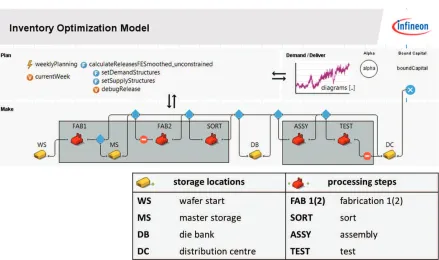
3.1 Snippet of the graphical user interface of the simulation model built with anylogic 28 3.2 Weekly planning of release quantities at the stock points in the simulation model 29 3.3 Illustration of the demand generation in the simulation model . . . 30

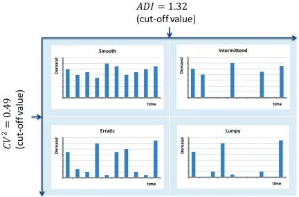
3.4 Illustration of the increasing uncertainty range over the simulation forecast . 31 4.1 Categorization of demand patterns according to Syntetos&Boylan [59] . . . . 36

4.2 Kolmogorov-Smirnov test . . . 45

5.1 Interaction between input, simulation model, and output. . . 49

5.2 biasSigma linear . . . 50

5.3 biasSigma concave . . . 50

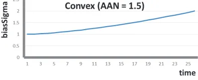
5.4 biasSigma convex . . . 51

5.5 Approach of finding the best demand parameter setting . . . 53

5.6 Kolmogorov-Smirnov approach . . . 55

5.7 Modified Kolmogorov-Smirnov approach for sales product 1 of basic type BT1 55 5.8 Relevant characteristics to be considered when improving the demand genera-tion method . . . 57

6.1 Customer order decoupling points at Infineon based on the illustration of [6]. 62 6.2 Time horizon of the production release approaches . . . 63

6.3 Various existing combinations for storing items at the stocking points in Infin-eon’s supply chain . . . 64

(18)

LIST OF FIGURES

6.5 α-service level versus total costs of the three production release approaches and

considered stocking strategies for basic type BT2 . . . 67

6.6 Change in the α-service level when decreasing the target reach at the master storage for each of the production release approaches of basic type BT1 . . . 69

6.7 Reduction in costs compared to the current costs when decreasing the target reach at the master storage for basic type BT1 . . . 69

6.8 Sensitivity analysis for BT1 . . . 72

6.9 Sensitivity analysis for BT1 . . . 72

B.1 Additive decomposition of time series data for product BT1 . . . 88

C.1 Autocorrelation for lags 1 to 20 of product 1 . . . 90

F.1 Graphical method of Welch for determining the warmup period on the example of the basic type BT1 . . . 100

H.1 Change in the α-service level when decreasing the target reach at the master storage for basic type BT2. . . 102

H.2 Reduction in costs compared to the current costs when decreasing the target reach at the master storage for basic type BT2 . . . 103

(19)

List of Tables

2.1 Plan cycle time for production steps of BT1 and its sales products . . . 15 2.2 Plan cycle time for production steps of BT2 and its sales products . . . 15 2.3 Summary statistics of delivered orders per week for basic type BT1 and its

three largest sales products . . . 21 5.1 Input parameters to demand generating function . . . 51 5.2 Relevant parameters for describing the demand behaviour, explanations are

based on [41] . . . 59 6.1 Experimental design for the simulation study of two exemplary basic types . 65 6.2 95% confidence intervals for theα-service level for basic Type BT1 . . . 70 6.3 95% confidence intervals for the costs andα-service level comparing the ‘Hist&Order’

with the ‘SES’ approach for basic type BT1 . . . 71 6.4 Example of production release in front end and incoming orders at the master

storage. . . 73 A.1 Correlation matrix for the six biggest sales products of the basic type BT1 . 87 C.1 Autocorrelation of first four legs for non autocorrelated and autocorrelated

demand . . . 91 C.2 One example of the first 30 periods out of 1040 periods for non autocorrelated

demand . . . 92 C.3 One example of the first 30 periods out of 1040 periods for autocorrelated demand 93 E.1 Chi-square statistic and critical value for the sales products of basic type BT1 96 E.2 Chi-square statistic and critical value for the sales products of basic type BT2 96 F.1 Number of replications according to the Replication/Deletion Approach for

(20)

(21)

Chapter 1

Introduction

Semiconductors are part of everyone’s daily life. When it comes to electronics such as smart-phones, power tools, medical systems, automobiles, robots and many more, semiconductor devices are an indispensable component of it. And still, the number of applications for mi-crochips is continuously growing since the transistor was invented in 1948. The competition among semiconductor manufacturers goes hand in hand with the increasing demand. Making it necessary for companies to not only offer their products at favourable prices but also to deliver on time [29]. Thus, companies strive for a competitive advantage through their supply chain management.

Infineon Technologies AG (Infineon), a German semiconductor manufacturer, usesdiscrete event simulation (DES) to continuously improve its supply chain and to remain competitive. Simulation depicts a system in a software based model with the purpose of understanding its behaviour or evaluating different strategies [56]. Hence, one aim is to reveal bottlenecks and deficiencies. By altering input parameters one tries then to remedy these weaknesses. As a result improved system settings are proposed.

A crucial factor of a simulation is its validity. Meaning that the simulation model has to reflect reality appropriately. This includes that the input data to the simulation model is accurate. Commonly, one generates input data which reflects observed values. This research supports Infineon to find a method that assesses the fit between observed and generated data such that the simulation input can be verified to reflect reality sufficiently. After evaluating the accuracy of the input data we further conduct a simulation study to improve the stocking strategies as well as the method of controlling the production start for two exemplary products of the Chip Card & Security division.

We start with briefly introducing Infineon insection 1.1 and continue by motivating the research topic insection 1.2. Then, insection 1.3andsection 1.4, we define the core problem and formulate the research questions which contribute to solving the problem. Last, sec-tion 1.5 describes the scope and limitations of our research and section 1.6 concludes the chapter with the Plan of Approach.

1.1 Company Introduction

(22)

CHAPTER 1. INTRODUCTION

and Power Management & Multimarket (PMM), where it holds leading positions. It strives for excellence by making life easier, safer and greener.

Main applications for Infineon’s products in CCS are microcontrollers for payment sys-tems, governmental identification documents, and sim cards to Gemalto, Oberthur, and G&D. ATV offers among others driver assistance and security systems such as airbags and ABS as well as general electronics like lighting and windowlifts. Customers include Bosch, Contin-ental, and Tesla. IPC focuses on electric engines, renewable energy as well as energy trans-mission and conversion for machines, locomotives, wind turbines, and solar collectors sold among others to Siemens and ABB. The PMM division provides chips for consumer goods for instance mobile devices, televisions, and computers, and sells these to large OEM’s and various large semiconductor distributors.

Infineon’s microelectronic revenues are about $6.5 billion with around 35,400 employees worldwide in the fiscal year 2016. This is allotted to 41% of Automotive, 17% of Indus-trial Power Control, 32% of Power Management & Multimarket, and 10% of Chip Card & Security [36].

The master’s thesis is conducted with the scenario & econometrics team of the corporate supply chain department at Infineon in Neubiberg. The team contributes to the success of Infineon by providing analyses and support services to the business divisions. This includes analysing trends and innovations over all four main markets and proposing interventions in the supply chain planning.

1.2 Research motivation

The key challenges faced by semiconductor supply chain management such as of Infineon include product variability (also refered to as product mix), demand fluctuations, long lead times, and a 24x7 production. These challenging issues influence the manufacturing efficiency, delivery performance, and volume elasticity considerably [9].

Product variability emerges due to the mere fact that product details are often customer specific. These may solely be slight changes or enhanced versions, however they alter the product noticeably. A reason for the rapid development of products is Moore’s law, which states that the number of transistors on an integrated circuit is doubling every two years [45]. Also, the wide spectrum of applications for semiconductors leads to a variety of products. Applications range from chips for smart cards, over microcontrollers for automobiles, to large power supplies in industry. Hence, semiconductor companies manufacture an immense range of products simultaneously. This product variability issue is aggravated by unpredictable demand, long lead times, and a 24x7 production at Infineon. Semiconductor companies are plagued by demand fluctuations due to their upstream position in the end-to-end supply chain. Before a semiconductor device reaches the end customer it moves along the supply chain, in our case from Infineon to distributor to customer. This fosters the Bullwhip effect that distorts demand information as it is transmitted up the chain. More precisly, demand variability increases when travelling upstream [43]. Due to the Bullwhip effect, firms in upstream positions cope with high demand fluctuations that impair controlling inventory, forecasting demand and scheduling production. Long lead times and a 24x7 production add up to this difficulty. The manufacturing process of integrated circuits takes up to three to four month. The process from the silicon raw material to the finished good comprises four main processes: Wafer fabrication, sort, assembly or packaging, and final test, some of these

(23)

including several hundred steps [29]. However, many costumers do not order three month in advance. Thus, to hedge against uncertainties semiconductor companies need to hold comparably large inventories [9]. These problems are strengthened by a 24x7 production at Infineon. A 24x7 production does not allow for volume flexibility, meaning that a high demand cannot be fulfilled by increasing production hours since production runs already continuously. Hence, incorrect volume planning cannot be remedied by working extra hours, but instead leads to delayed deliveries, which in turn reflect a poor delivery performance.

To hedge against manufacturing inefficiency, demand uncertainty, and missing volume elasticity Infineon places stocks at various stocking points in its supply chain. To help the divisions improve their stocking strategies Infineon’s flexibility & econometrics team uses discrete event simulation. Usually, the different strategies are evaluated according to the trade off between the α-service level and the costs.

1.3 Problem definition

In a former project Infineon’s flexibility & econometrics team performed a simulation study for a group of products of CCS which showed that stocks can be reduced drastically. In this project we continue the successful collaboration with the CCS division. They are interested in analysing various stocking strategies and production release approaches for two particular products. That is, we try to answer the following questions:

stocking strategy:

1. At which stocking locations to place inventory in the supply chain? 2. How high should the inventory be at these locations?

production release approach:

3. How to quantify the amount of wafers to be released to production in advance? The two products are of relevance for CCS due to their high production volume and revenue share of more than 25% of CCS’s total revenue. To provide CCS with answers to these questions, we use the existing simulation model. It was built by the scenario & econometrics team and further enhanced as part of a master’s project such that it allows for flexible product structures [13]. It is described in more detail in chapter 3. With the simulation model we are able to run various experiments where we alter the stocking strategy and the production release approach.

A key part of a simulation study is to have accurate input data. That is, the generated data should be similar to the observed data. Otherwise, results are misleading and proposed solutions do not show the same behaviour in reality as they do in simulation. Currently, there is no established method at Infineon to validate the generated input data according to the observed input data. As part of this project, we require to find a method that assesses the fit between the generated and observed data.

(24)

[image:24.595.85.524.110.340.2]

Figure 1.1: Production start according to forecast and further processing on basis of customer orders

differ since the forecast represents a moving average and the demand refers to the actual orders customers place. Figure 1.1presents where in the supply chain the marketing forecast and the customer orders are employed. For the products we are considering, the marketing forecast is used to start the production of unprocessed wafers up to the diversification point (master storage). Hence, the current production release approach is based on the marketing forecast. Whereas the customer orders are used to start the production of the pre-processed wafers from the diversification point onwards. The chips become customer specific and are waiting at the distribution centre for delivery to the customers.

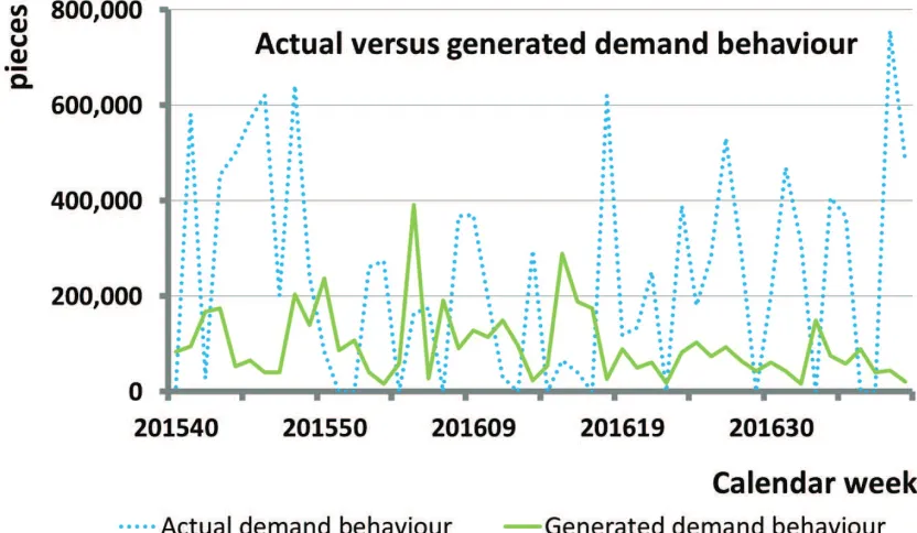
The simulation model generates the customer orders. To receive valid simulation results, we require that the generated data resembles actual customer order data such that their characteristics are similar.Figure 1.2shows an example of actual and generated demand data. There exists various techniques in the literature to compare two time series and assess their fit. For example, we can use forecast accuracy measures such as the MAE (Mean Absolute Error), the MAPE (Mean Absolute Percentage Error) and the SMAPE (Symmetric Mean Absolute Percentage Error). These measures compare a forecasted value at time t with the observed value at timet. The difficulty with these measures is that they compare two points with one another and do not consider the overall behaviour of the time series. However, we are rather interested in a statistical equivalent behaviour than in the exact values. The advantage of having a statistical equivalent behaviour is that we can generate various realisations of this demand behaviour and use it for several simulation runs. This ensures that the output is not only based on one realisation but on many and thus reduces the effect of outliers. Hence, we want to find a method with which we can assess the fit between two time series regarding their statistical behaviour.

Our procedure is as follows. We parametrize the arrival processes in the given simulation model such that the generated data represents observed data according to our defined method.

(25)

[image:25.595.86.502.117.359.2]

Figure 1.2: Example of actual versus generated demand data

Next, we use the adjusted simulation model to study the two products of CCS. This regards various stocking strategies and production release approaches which are evaluated according to the service level as well as respective costs. We aim to find the set up that improves the supply chain planning of CCS.

In summary, we can formulate the core problem in the following statement:

Improve the supply chain planning process according to the service level and respective costs at CCS for two particular products considering the stocking strategies as well as the approach of quantifying the amount of wafers to be released to production.

To be able to solve this core problem we need to solve the two subproblems below which are strongly interconnected with the core problem and thus are highly emphasized. These are:

Parametrize the order arrival process in the existing simulation model such that the generated demand data correctly describes the observed data to make the simulation results more representative.

Define a method to assess the fit between generated and observed values according to their statistical behaviour.

(26)

1.4 Research problem

1.4.1 Research goal

Currently Infineon does not have an established method that assesses the fit between the historical demand and generated demand data. In order to receive valid simulation results the input to the simulation model has to reflect observed values correctly. A key prerequisite of the method is its ease of use. Consequently, the goal of this research is, firstly, to parametrize the arrival process such that it models the true behaviour of representative products, secondly, to construct a method which assesses the fit between generated and observed data, and thirdly, to conduct a simulation study for two exemplary products of CCS. This simulation study aims to consider various stocking strategies as well as approaches to quantify the amount of wafers to start in production in order to give alternatives to the current practice.

1.4.2 Problem statement

The problem statement is formulated to generate the needed knowledge.

‘How can Infineon assess the fit between the generated and observed demand data for representative products of the CCS division and para-metrize the simulation’s arrival process to obtain valid results?’

We want to exploit existing techniques to evaluate the fit between two time series. Values at time t of the generated data do not need to match values of the observed data at time t

exactly, but we aim to assess whether the overall behaviour of the series is statistically similar.

1.4.3 Question formulation

To tackle the problem statement, we formulate several research questions. Each research question including its sub questions corresponds to a chapter of this thesis. These research questions will be answered by interviews with employees of Infineon, reviewing available liter-ature, performing an elaborative data analysis, developing a method to evaluate the behaviour qualitatively and conducting a simulation study.

Current situation.

First, we obtain in-depth knowledge of the current situation. For this purpose we look at two domains, the broader context and the data of the considered products. The context involves gathering information about how supply chain planners at CCS define production volume, which data sources are used and how orders influence the production start. In addition, we look closer at the data of the representative products and conduct an analysis to identify patterns.

1.1) How is the supply chain planning carried out? a) How is the supply chain set up?

b) Which products are representative and appropriate to consider? c) Which data sources are used for storing the demand data at CCS? d) How do orders and forecasts influence production start?

1.2) How does the demand data of the representative products from Chip Card & Security behave?

(27)

a) What patterns can be identified in the data?

b) Which statistical measures are important to consider? Simulation model.

We use discrete event simulation to analyse various system settings. Thus, we explain the methods, inputs, and outputs of the existing simulation model.

2) How is the simulation model set up?

a) What is the purpose of the simulation model?

b) What is the structure of the model, e.g. logic, input and output parameters? c) How does the simulation model work?

d) What are the input and output parameters of the simulation model? Literature review.

We continue with a literature review to study existing approaches concerning how data series can be compared. Several approaches exits in literature which concern among others forecast accuracy measures, time series similarity measures, and hypothesis tests. This lays a foundation to assess our arrival process which should model observed demand behaviour appropriately.

3) What solution approaches exist in literature to assess the fit between generated and observed demand data?

a) How can two time series be compared?

b) What are the advantages and disadvantages of these measures and methods? Parametrization and fit between time series.

The next step is to parametrize the arrival process of the simulation model to generate demand data which represents the behaviour of the observed data. Moreover, we apply a suitable method to assess the fit between two time series based on the findings of the literature review.

4) How do we need to parametrize the simulation model to create accurate demand data?

a) What input parameters are relevant?

b) How accurately does the generated data fit to the observed data?

c) How can we improve the fit between the historical data and the generated data?

Simulation study and Evaluation.

The simulation study is performed in order to assess several stocking strategies and pro-duction release approaches for the analysed products of CCS. To compare the various ap-proaches we need to define key performance indicators (KPIs). The results of the simulation study serve as an indication how CCS can improve their supply chain planning process. We conclude the thesis with recommendations and an outlook.

5) How can the planning process of CCS be improved? a) Which strategies can be used to start production? b) Which stocking locations should be used to store items?

(28)

1.5 Research Scope and Limitations

Due to time constraints of this research project and some limiting factors we narrow down the scope and mention simplifying assumptions.

As introduced earlier, Infineon is structured in four divisions, all of which provide a wide range of products. Since time constraints do not allow considering all products, we will focus on two exemplary products from Chip Card & Security (CCS). We restrict our selection to products of CCS for the reason that these products show a volatile behaviour, whereas products from for example ATV are rather stable in their demand patterns. Furthermore, the existing simulation model is built on the supply chain specifics of products from CCS. Hence, major modifications of the simulation model will not be required.

We can omit the validation of the simulation model since it was validated by a previous master’s thesis that enhanced the used model [13]. By valid we mean that the physical supply chain is mapped well enough in the simulation. The focus solely lies on adjusting the existing model with an accurate parametrized demand and forecast signal, however, we do not focus on the process steps in the simulation to accurately represent the supply chain.

In addition, we differentiate this master’s project from a previous project which was also done with Infineon’s flexibility & econometrics team in cooperation with the Faculty of Behavioural, Management and Social scienes of the University of Twente [1]. The previous project considered the trade off between the utilisation of machines and the resulting costs of storing inventory. A higher utilisation of machines leads to a higher cycle time due to a higher work in process (WIP). The focus lied on improving the accuracy of the simulation model. In contrary, in this project we concentrate on the trade off between the service level (associated with high stocks) and the respective costs without considering machine capacity. Moreover, we focus on adapting the simulation model according to two particular products to improve their planning process.

1.6 Plan of Approach

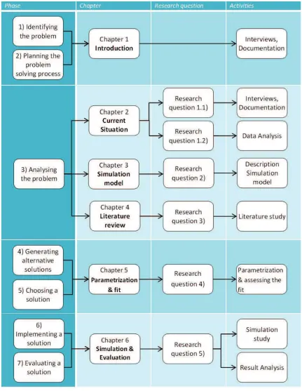
A well-known approach of structuring and solving research is the Managerial Problem Solving Method (MPSM). The method intends to solve an action problem as identified insection 1.3, which states to improve the supply chain planning process of Infineon and thereby modelling demand behaviour according to observed values. The MPSM is composed of various phases.

1. Identifying the problem

2. Planning the problem-solving process 3. Analysing the problem

4. Generating alternative solutions 5. Choosing a solution

6. Implementing the solution 7. Evaluating the solution

Figure 1.3below maps these phases to the chapters of the thesis to give a brief overview of the structure and determine the activities for each step.

(29)

[image:29.595.80.511.133.690.2]

(30)

(31)

Chapter 2

Current situation

To start with, section 2.1introduces the supply chain process of Infineon and goes into more detail regarding the planning of CCS and its products which we simulate later in this project to improve their stocking levels. In section 2.2, we continue with a data analysis that serves as a basis for modelling the arrival process of the demand and forecast in the simulation. The focus of the data analysis lies on two high runner products.

2.1 Current Situation

2.1.1 General description of Infineon’s supply chain and its planning

In order to manage its supply chain processes Infineon implemented the Supply Chain Oper-ations Reference Model (SCOR), which is a management tool recommended by the APICS Supply-Chain Council. It describes the business activities associated with five distinct phases to satisfy customer demand [19]. The phases are: Plan, Source, Make, Deliver, and Re-turn. Figure 2.1 shows how these five phases of the SCOR model link to Infineon’s supply chain.

We focus on the activities of theplan and make process which are relevant for our simu-lation study and only give a brief description of the other three phases. The discussion in the remainder of this section refers to the internal documents [19,55] of Infineon. Theplanprocess is responsible for balancing the available resources with the given requirements. The source process takes care of the deliveries from internal and external suppliers, including purchasing activities as well as sourcing logistics. The make process includes the main production steps of the supply chain, namely fabrication, sort, assembly and final test. The deliver process concerns all sorts of deliveries to internal and external customers and thereby taking care of order management, and invoicing customers. Last, the return process deals with products that are either returned by Infineon to its suppliers or by customers to Infineon [19].

The Plan process.

(32)

[image:32.595.82.518.113.280.2]

CHAPTER 2. CURRENT SITUATION

Figure 2.1: SCOR model linked to Infineon’s supply chain [19]

Figure 2.2: Plan processes at Infineon [55]

management and a constrained forecasts, that is, the amount Infineon can sell considering available machine resources, for order management. Last, 4) the production management as well as 5) the order management establish and communicate plans for production and customer deliveries, respectively.

There are two major activities in the demand planning process on the operational level regarding our simulation study. First, the generation of a forecast of what Infineon could sell into the market in number of pieces per week. We aim to model this weekly forecast data in the simulation model to increase the model’s validity. Second major activity is the definition of the target reach for the stocking points. The target reach is defined as the safety stock in number of weeks. That is, the supply chain planner determines how much to store at the various stocking locations for each product. Stocks are needed for three main reasons:

1. Uncertainty in demand and production 2. Long cycle times

3. Strategic decisions

Demand uncertainty occurs due to varying orders of customers and production uncertainty occurs due to machine downtime which varies the cycle time. Stocks are built to hedge against

(33)

these uncertainties. In addition, cycle times are quite long due to a complex manufacturing process. To be able to respond quickly to customer demand, stocks are needed to reduce the lead time. Moreover, stocks are necessary when production gets transferred to another production location. E.g., production may be transferred from location 1 to location 2, however, customers may require to further receive their products from location 1 since they solely certified location 1. Thus, we need to build up stocks for these customers with products of location 1.

We intend to improve stocking levels and the approach of quantifying the amount to start in production by conducting the simulation study because it is important that stocks are neither too low nor too high. If stocks are too low, master storage and diebank products are missing and customer orders cannot be confirmed. As a result Infineon loses revenue and dissatisfies its customers who may move to competitors. On the other hand, if stocks are too high, Infineon invests in unnecessary products and hence raises the bind capital. Moreover, it increases the risk of scrapping master storage products, die bank goods and fin-ished products [55]. This situation can be described by the trade off between the service level and costs. A high service level indicates comparably high stocks and thus also high costs, whereas low stocks are associated with a lower service level and also lower costs. The aim is to balance this trade off.

The Make process.

The main result of the make process is the finished product, namely the silicon chip or microchip. Making silicon chips is one of the most complex manufacturing tasks. It is grouped into front end and back end, taking between 40 and 100 days (6-15 weeks), and up to 20 days (3 weeks), respectively. In the front end chips are produced onto the silicon wafers. In the back end wafers are diced into single chips. These single chips are equipped with an outer package containing pins or a conductive surface to connect with other electronic components. Both processes are separated by the die bank. Figure 2.3 gives a schematic overview of the process and possible stocking points, similarly to the existing simulation model.

Wafers are produced from raw silicon, which builds the basis for microchips. Silicon is used due to its properties as a semiconductor. Depending on the treatment it either conducts or blocks the flow of electricity making it ideal to function as a transistor.

(34)

[image:34.595.96.509.107.396.2]

Figure 2.3: Make process at Infineon [55]

capacities more products than requested may be produced. At the assembly wafers are cut into individual chips and in the die bonding a package is attached to the chips. It is followed by the wire bonding, where interconnections between the integrated circuit and its package are made. Finally, the chips are moulded, trimmed and formed. Now they are ready for the last quality check, the Burn-in testing. It stresses the component under supervision to detect defective chips. Chips which fail this test are sorted out. The last part of Infineon’s supply chain forms the distribution centre (DC). At this stocking point finished products are stored before they are transferred to the customers [19]. Typically, there is no stock at the distribution centre for make-to-order products. However, customers may request to have finished products at the distribution centre or products may be stored temporarily before delivery [37].

Thecycle time (CT), defined as the length of time spent by a product unit in the system from the release of the wafer into the fabrication until finishing the last step in the test takes up to four month without considering storage time in the master storage or die bank. Two to three months are allotted to the front end and roughly one month is allotted to the back end. These long cycle times especially in the front end indicate that it is necessary to use forecasts up to the master storage and die bank such that customer orders can be fulfilled quickly in order to stay competitive.

Infineon’s supply chain process is spanned over a global network, meaning that there are various production and stocking locations spread all over the world. Front end facilities are among others in Dresden (Germany), Regensburg (Germany), Villach (Austria) and Kulim (Malaysia) and external suppliers include the Taiwan Semiconductor Manufacturing Company

(35)

Table 2.1: Plan cycle time for production steps of BT1 and its sales products

Basic type BT1 Front End BackEnd

Productionstep FAB SORT ASSEMBLY TEST

Facility: CT in day Dresden: 91 Dresden: 18 Regensburg: 7 Regensburg: 0 TSMC: 91 ADT: 7 Wuxi: 7 Wuxi: 0 Table 2.2: Plan cycle time for production steps of BT2 and its sales products

Basic type BT2 Front End BackEnd

Productionstep FAB SORT ASSEMBLY TEST

Facility: CT in day Dresden: 70 Dresden: 14 Amkor: 9 Amkor: 7 TSMC: 70 ADT: 4.5 Regensburg: 7 Regensburg: 0

Wuxi: 7 Wuxi: 0

(TSMC, Taiwan) and Ardentec (ADT, Taiwan). Back end facilities are located among others in Regensburg (Germany), Warstein (Germany), Malacca (Malaysia) and Wuxi (China). Ex-ternal partner is for instance Amkor Technology (United States of America). The die bank locations are either based at the front end or the back end facilities [19].

2.1.2 CCS’s high runner products

Chip Card & Security (CCS) focuses on products in three main areas: payment systems, governmental identification documents and mobile communication [36]. The two products we are considering, BT1 and BT2, belong both to payment systems. Product BT1 is a chip for contactbased payment integrated in credit and debit cards and BT2 is a chip for contactless payment also integrated in credit and debit cards. Other payment systems are mobile payment and NFC-based contactless payment. Products BT1 and BT2 are of main interest, since they contribute to CCS’s yearly total revenue by >25% and have a high production volume. [31]. As we introduced Infineon’s supply chain in the previous section, we give here some further information of the two products.Table 2.1andTable 2.2summarize the specificCTsin days per production step and also depict the facility locations where the treatment takes place. When production is started at the fabrication we speak ofbasic types. BT1 and bp are both basic types. In the sort step these two basic types receive customer specific information and are then identified as sales products. A basic type can serve as a basis for several hundreds sales products. In our case, 95 different sales products are made from basic type BT1 and about 180 sales products are made from basic type BT2. Later, we solely consider the largest sales products of each basic type which account for _≥ 85% of the total volume. These are six sales products for BT1 and ten sales products for BT2. Customers order on sales product level [37].

(36)

Figure 2.4: Delivery reliability at Infineon

time sums up to roughly four months, where a large part of about three and a half months is allotted to the front end and only a small part of about two weeks is allotted to the back end. Hence, it is significant to plan the right amount of stocks in the front end stocking points, master storage and die bank, to decrease the lead time and fulfil demand quickly. Otherwise, if production is started when orders arrive, lead times are too long for a highly competitive market. Basic type BT2 is processed at the same locations in front end and back end with similar cycle times. Next to the back end locations, there is also a facility of Amkor with a slightly higher cycle time which is due to their internal production process.

Clearly, the amount of produced products is dependent on the customer demand. As mentioned earlier, we distinguish between actual customer orders and marketing forecast. A customer order is a request by a customer for a certain amount of one or more customer specific products containing a delivery wish date. Customer orders are produced up to the distribution centre. A marketing forecast, on the other hand, is an approximation of what and how much a customer may order in the future and is done by marketing using a four month moving average over the historical orders. Marketing forecasts are produced up to master storage. This is done in order to decrease the lead time as the cycle time at the frontend can be omitted when orders are produced from master storage. There are no products produced on forecast to the die bank or the distribution centre, since die bank and DC products are customer specific and the risk of scrapping products is too high [31,37]. Currently, the amount of wafers at the master storage cover atarget reach of 13 weeks.

The performance of the current approach, which defines the release quantity in front end by a four months moving average with a target reach at the master storage of 13 weeks is measured at Infineon by thedelivery reliability (DR). TheDRis an internalkey performance indicator (KPI)which is calculated for each product. A delivery is considered to be reliable if theproof of delivery (POD)is a date between the customer’s wish date minus some delivery window and the first confirmed delivery date by the supply chain planner plus some delivery window as shown in Figure 2.4.

The current delivery reliability for the products BT1 and BT2 is 93%. Note that, the current simulation model does not include a method which captures the interaction between the supply chain planner and the customers such that theDRcan be measured since it would

(37)

introduce a higher level of complexity and may reduce the runtime of the simulation model. Instead, in order to prevent unnecessary high complexity the α-service level is implemented in the simulation model. It is chosen since it captures the idea of theDRwithout introducing further complexity. Similarly to the DR, the α-service level becomes either 0% when not all demand is met by on-hand inventory or it becomes 100% when all demand is met by on-hand inventory explained in detail in section 3.3.2. Note that, backorders are not taken into account. Since we have given the delivery reliability but not the α-service level, we need to find the α-service level that corresponds to the DR of 93%. This is done by using the current simulation model. The simulation model was verified by [13], thus we can determine the current α-service level by running the simulation for both basic types with a target reach of 13 weeks at the master storage and a four months moving average over historical data to determine the release quantity. This results in an α-service level of 98%.

2.1.3 Stocking policy approaches at Infineon

Infineon uses various approaches to plan stocking levels at the master storage, die bank, and distribution centre ranging from basic approximations to advanced simulation-based methods thereby increasing the quality of the proposed solution along with the effort. The following discussion based on [21] shows how we classify our project.

A basic approach on a high aggregation level is using a rule of thumb. The supply chain planner estimates the target reach according to his experience and uses the estimated value for all products. Thus, there is no differentiation between products nor fluctuations over time are considered. Nevertheless, it is easy to apply.

To add more detail,ATVintroduced the ‘Enhanced Inventory Planning’ for some of their products. At this level of detail, products are considered separately and the target reach is calculated for the various stocking points by using an echelon stock policy. An echelon stock policy is characterized by central control and the visbility of customer demand in the entire network. An installation stock policy, on the other hand, is characterized by local control and the demand at each stocking point is based on the demand from the downstream stockpoints [6]. For the calculation general inventory models such as the (R, S) policy are used, where every R periods (weekly) an order is placed to rise the inventory position to the order-up-to level S. In order to apply these inventory models, usually the assumptions of a normal distributed demand as well as the independence of succeeding time periods are made, where demand of one period has no influence on demand of a subsequent period [6]. A normal distributed demand facilitates computations and gives a good approximation when demand is high enough [61]. Note that, there exist extensions in the literature in case of non-normal demand and dependent time periods. Fortuin examines five different probability density functions for the demand (Gaussian, logistic, gamma, log-normal, Weibull) [25]. He finds that except for the logistic distribution expressions are much more complex. Burgin further investigates on the Gamma distribution and devotes considerable effort to develop approximations [10]. In addition, other distributions such as Poisson [57], Laplace [51], and Negative binomial [20] have been studied. For a further listing and according references we refer to [57]. A short discussion is also provided in section 5.3. The described approaches are analytical methods to define the order-up-to level S for the stockpoints in multi-echelon in-ventory systems. It is advisable to use analytical methods when computations are comparably easy and assumptions such as a stable average demand rate are met [41,57].

(38)

com-CHAPTER 2. CURRENT SITUATION

plex relationships and detailed structures are modelled as well as when time depending events occur. Simulation allows to explicitly model the relation between products, machines, and operators. That is, different products may have different processing times and different routes through the system. These may further be influenced by various operators. Simulation also allows to include variability in processing times due to machine downtime. In addition, the product structure (basis product splits up into several specific products) can be included in a simulation model with the according demand for the specific sales products. Moreover, even though discrete event simulation implies with its name that events occur at discrete time steps, we can easily vary at which time steps to execute an action, e.g. every time step, every second time step or make it dependent on some conditions. Furthermore, another advantage is that actions can be triggered depending on certain conditions, which may be varying itself. Last, a practical upside of simulation is that processes and changes over time can be shown in graphs and moving figures. This facilitates the understanding of the system behaviour and the communication with management. Thus, using simulation allows for higher flexibility than analytical methods. However, it also requires a higher amount of effort and detail.

Since the manufacturing process of Infineon is highly complex with interactions between various processing steps, variability in the demand and processing times as well as a complex product structure and on the other hand, there is already an existing simulation model for the process of products from CCS, we decide to use discrete event simulation. Specifying the approach of simulation, our aim is to parametrize the demand generation method in the existing simulation model such that it reproduces the behaviour of observed demand precisely. Hence, we require to assess the fit between the generated and observed demand by a suitable method. With the enhanced simulation model we aim to improve the target reach, that is the stocking strategies as well as the production release approach, which is currently based on a four months moving average. The used key performance indicators (KPI) to measure the performance of the strategies are the service level and the costs, which we explain in section 3.3.2.

2.2 Data Analysis

We choose simulation to improve the supply chain process of CCS. To receive valid simulation results, the input to the simulation model has to reflect reality well enough. Thus, we conduct a comprehensive data analysis using Excel and the statistical software R to learn about the data’s behaviour. R is used in addition to Excel since it has the advantage of various build in functions such as statistical tests and is able of coping with large data sets. To start with, we gather several data sources and select one based on its completeness and validity. Next, we give a numerical and graphical summary of the data. In addition, we attempt to decompose the time series into a trend, seasonality, and error term. As this fails to recognize a suitable trend or seasonality, we further consider the autocorrelation of the time series to detect whether there are succeeding periods of increasing/decreasing demand. Having several periods with an continuously high demand rises the probability of stock outs. Thus, we conclude that autocorrelated data behaves differently to non autocorrelated data. That is, if the generated data is autocorrelated, but the historical data is not or vice versa, wrong conclusions from the simulation results may be drawn.

(39)

2.2.1 Demand patterns

We gather and consolidate several data sources in order to have a complete and valid repres-entation of customer orders. The below mentioned requirements ensure that the data source is representative:

1. Data should be on a weekly basis.

2. Data should contain data points over a minimum of 52 weeks. 3. Data should contain the requested quantities per sales product. 4. Requested quantities by customers should be represented in pieces. 5. Data should contain the due week of the order.

Since planning of customer shipments occurs on a weekly basis we require the level of data to be weekly as well. Further, we opt for a time span of minimally 52 weeks to have a data set that has enough data points to draw conclusions and represents patterns sufficient. Next, customers order the sales products in number of pieces. Last, we require the due week of the orders that customers request such that we can represent how demand occurs over time and to identify dependencies between time periods.

For the validation of the data sources we compare the revenue figures ine_{with the annual}

report for the fourth quarter of the fiscal year 2015 and the first three quarters of 2016. We assume that comparing the revenue figures of the available data sources with the annual report is suitable to determine whether the data is complete and contains all sales. This comparison shows that one out of three potential data sources is sufficient for further analysis as it differs only by 2%, whereas the other data sources differed by more than 15% due to missing and incomplete data. The sufficient data source is called data mart order processing (DMOP).

The maximum difference between the data of DMOP and the annual report on a quarterly basis is 3% and the minimum is roughly 0%. Aggregating the numbers on a yearly basis res-ults in a difference of about 2%. The difference may be due to returned orders or when actual payments fall into another quarter. We assume that this represents the demand well enough. Regarding the above defined requirements, the DMOP data fulfils conditions 1 to 4. However, it does not fulfil condition 5, that is, the due week as requested by the customer is not contained in the data. Nevertheless, it contains the week the order was delivered at the customer site. We assume that this is sufficient to represent the demand for a certain week and hence neglect the case that orders are delivered deviating from the due week.

Demand behaviour on the example of basic type BT1.

On the example of basic type BT1 we present the results of our data analysis which aims to provide us with a better understanding of the data and its behaviour. The data analysis was done using Excel as well as the statistical software R. The graphical summary of basic type BT1 is plotted in Figure 2.5. It represents the orders in pieces per week over two years, from January 2014 to December 2015. One can see that the deliveries increase over time and that they are fluctuating. The increase over time is due to the product life cycle which suggests that demand grows until it matures and eventually levels off [31].

(40)

[image:40.595.86.511.112.324.2]

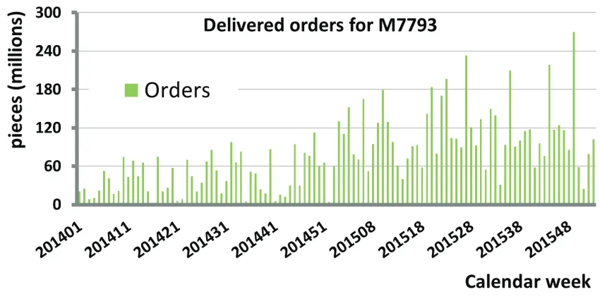
Figure 2.5: Delivered orders of BT1 in pieces (millions) per week from January 2014 to December 2015

which make up _≥ 85% of the total volume. The mean demand of the basic type over the two years is about 10 million pieces per week with a standard deviation of around 6 million pieces. When calculating the coefficient of variation (CV), which indicates the dispersion of data points, we receive a value of 0.61. It means that the deliveries are fluctuating since theCV is>0, however these fluctuations are not very large. Moreover, the median lies with about 8 million pieces comparable close to the mean demand and therefore suggests that the distribution of the values is not skewed to the right or to the left but rather symmetric. Last, we classify the demand pattern by the scheme of Syntetos & Boylan [59] described in subsec-tion 4.1.1. We choose this categorization since it can be applied independent of the empirical data set. The basic type is classified as smooth meaning that it has moderate fluctuations and constantly occurring demand. This implies for the planning that the production release in front end can be rather stable.

Looking closer at the data, we consider the largest sales products of the basic type BT1. In total 95 sales product (SP) are manufactured on basis of this basic type. The largest three sales products, SP1, SP2 and SP3, account for 39%, 24% and 9% over the two years, respectively. When looking at the data of 2015 only, the amount of the three sales products even increases to a total of 91%. SP1 has a mean of about 4 million pieces per week over the two years per week , SP2 has a mean of about 2 million pieces and SP3 has a mean of about 1 million pieces. The median for SP1 lies close to the mean suggesting that there are no big outliers and that the distribution is rather symmetric. However, the median of SP2 and SP3 is zero, meaning that over the two years in 50% of the weeks there are no orders delivered. This also implies that the distribution is skewed to the left. Furthermore, the coefficient of variation for all three products shows that SP1 has a smaller relative variability compared to SP2 and SP3, where SP3 has the largest relative variability. However, the variability of all three sales products is still noticeably. This is in accordance with the classification in erratic for SP1, and lumpy for SP2 as well as SP3. The erratic and lumpy demand patterns are both

(41)

Table 2.3: Summary statistics of delivered orders per week for basic type BT1 and its three largest sales products

BT1 SP1 SP2 SP3

Mean 9,916,641 3,876,597 2,388,385 897,302

Median 8,501,889 3,791,629 0 0

Standard Deviation 6,090,168 3,362,978 3,747,042 1,513,485

Minimum 1,020,868 0 0 0

Maximum 28,130,769 11,338,889 14,961,713 9,795,001

CV 0.61 0.87 1.57 1.69

Classification of

Syntetos & Boylan smooth erratic lumpy lumpy

characterised by fluctuating demand, while demand occurs frequently in the case of an erratic classification but rather seldom in case of a lumpy classification. Erratic demand patterns imply for the planning that forecasts of demand should not be based solely on one demand point as this may lead to large over- and underestimates. On the other hand, for the planning of lumpy demand Croston [14] suggests to analyse the volume of the non-zero demand and the interval between successive non-zero orders separately. Thus, two forecasts are made, one for the volume of the order and one for when the next order will occur.

Last, we consider the correlation among the sales products to check whether there are any dependencies among them. The Pearson correlation coefficient for two samples X and Y is defined by [64]

rX,Y =

Pn

t=1(xt−x¯)(yt−y¯) pPn

t=1(xt−x¯)2pPnt=1(yt−y¯)2

(2.1)

The analysis shows that the sales products are not correlated among each other. Results can be found in Appendix A.

Times series decomposition for BT1.

Time series decomposition is a classical method of time series analysis. It tries to discover patterns in the historical data and extrapolates these into the future. In contrast, regression analysis aims to reveal an explanatory relationship between one or more independent variable and the output [22]. We focus on time series decomposition as we are interested in the patterns and not in an explanatory relationship. Time series decomposition breaks down a time series into subpatterns that identify separate components. This gives the analyst a better understanding of the series, and improves accuracy in forecasting since suited forecasting models can be chosen on the obtained information. Thereby, it assumes that the data is a function of a trend-cycle, seasonality and an error term [22,33]:

(42)

1. Estimating the trend-cycle.

2. Removing the trend-cycle component. 3. Estimating the seasonal component. 4. Estimating the error term.

Time series data is often described by a non-stationary process. For a non-stationary process the mean and/or the variance change over time whereas a stationary process has the property that the mean and variance are constant and do not change over time [8]. Clearly, if there is a trend in the data the series is non-stationary as the mean changes over time. However, many models assume stationarity. Stabilizing the mean can be achieved by either differencing or de-trending the series, stabilizing the variance can be achieved by log-transformation of the data [33]. To detect non-stationarity various statistical tests such as the Dicker-Fuller tests exist in literature.

As we found that the variance does not change significantly over time, we do not need to stabilize it. A stabilization of the mean beforehand is also not necessary as it is part of the decomposition to remove the trend of the data. The trend-cycle is estimated by calculating an appropriate moving average. For instance, when data is monthly a 12th _{order centred} moving average can be used to represent how the data develops over a year. Similarly with daily data, we calculate a 7th order moving average to show the trend over a week. Since our data is weekly we would assume to calculate a 4th _{order centred moving average to} ag-gregate the data over a month. However, this results in a random pattern that cannot be described as a trend. Therefore, we increase the order of the moving average such that more data points are aggregated and thereby smoothing the trendline. This results in a 26th _order moving average of our weekly data meaning that we aggregate data points over six months in order to detect a smoothed trend. It is reasonable to use a 26th order moving average since the planning horizon is also 26 weeks. Next, we detrend the data by subtracting the trend from the time series. This leaves us with the seasonality and an error term. The seasonal component is estimated by calculating a seasonal index per week over the two years since the data is weekly. From the plot shown in Appendix B, one can see that there is no seasonality recognizable. Hence, we can conclude to detect a trend the data needs to be smoothed by aggregating it over at least six months otherwise a random pattern is drawn and there is no recognizable seasonality in the data.

2.2.2 Autocorrelated demand data

Erkip et al. [23] find that autocorrelation is important to detect consecutive periods of in-creased demand. In case of positive autocorrelated demand safety stock needs to be higher to attain the same stock out probability than in case of non autocorrelated demand. Thus, we are interested in investigating whether the observed demand shows autocorrelation.

Autocorrelation of basic type BT1.

The autocorrelation measures the internal dependency of a time series between two time periods [8]. Similarly to the correlation coefficient, which measures the dependency between two variables, the autocorrelation gives a value between -1 and 1 for highly negative and highly positive correlated values, respectively. In contrast, values close to 0 indicate that there is no correlation, that is, time periods are independent.