Numerical Simulation on Interface Instability under Reshock

U

NIVERSITY OF

SCIENCE AND

TECHNOLOGY OF

C

HINA

& UNIVERSITY OF

TWENTE

I

FINALREPORT

Numerical Simulation on Interface Instability

under Reshock

Author

C.F.C.VANWIJK

Supervisors

Prof. Harry HOEIJMAKERS Prof. Xisheng LUO Dr. Juchun DING

Contents

Abstract 3

1 preface 3

2 Introduction 3

3 Problem Analysis 5

3.1 Assignment description . . . 5

3.2 Theory and analysis . . . 5

3.2.1 Richtmyer-Meshkov Instability . . . 5

3.2.2 Single-mode RMI . . . 8

3.2.3 RMI under reshock . . . 9

3.2.4 Dimensionless RMI . . . 10

3.2.5 Multi-mode RMI . . . 11

3.2.6 Current research into reshocked RMI . . . 11

3.3 Goal and Hypothesis . . . 12

4 Approach & Method 13 4.1 Research cases . . . 13

4.1.1 Recreating the simulation research by Latini et al. . . 13

4.1.2 Single-mode RMI simulation comparison to experiments . . . 14

4.2 Verifying mesh size . . . 15

4.3 Effects of various parameters . . . 15

4.3.1 Reshock time . . . 16

4.3.2 Wavelength . . . 17

4.3.3 Initial amplitude . . . 17

4.4 Mach number . . . 17

4.5 Research method . . . 18

4.5.1 MZ amplitude . . . 18

4.5.2 Bubble and spike amplitude plots . . . 18

4.5.3 Schlieren images . . . 19

4.5.4 Fourier mode analysis . . . 19

4.6 HOWD simulation tool . . . 19

5 Results & Discussion 23 5.1 Recreating the two research cases . . . 23

5.1.1 Simulation by Latini et al. . . 23

5.2 Comparison to physical experiments and base case selection . . . 25

5.3 Mesh size verification . . . 27

5.4 Varying parameters . . . 28

5.4.1 Reshock time . . . 28

5.4.2 Wavelength . . . 30

5.4.3 Initial amplitude . . . 32

5.4.4 Mach number . . . 34

5.5 Results of FFT analysis . . . 36

6 Conclusions & Recommendations 41

7 Acknowledgements 43

Appendices 45

A Paper reviews 45

A.1 Growth rate predictions of single- and multi-mode

Richtmyer–Meshkov instability with reshock . . . 45 A.2 Experimental and numerical investigation of the Richtmyer–

Meshkov instability under re-shock conditions . . . 47 A.3 Reshocked Richtmyer-Meshkov instability: Numerical study and modeling of

random multi-mode experiments . . . 49 A.4 Physics of reshock and mixing in single-mode

Richtmyer-Meshkov instability . . . 53 A.5 High-resolution simulations and modeling of reshocked

single-mode Richtmyer-Meshkov instability: Comparison to experimental data and to amplitude

growth model predictions . . . 53 A.6 High-order WENO simulations of three-dimensional reshocked

Richtmyer-Meshkov instability to late times: Dynamics, dependence on intitial condi-tions, and comparisons to experimental data . . . 57

B Schlieren images of the SM RMI experiments by Liu et al. and HOWD simulation 61

C Schlieren images of different mesh size cases 66

D Schlieren images for different reshock times 68

E Amplitude plots for different reshock times 70

F Schlieren images for different wavelength cases 72

G Amplitude plots for different wavelength cases 73

H Schlieren images for different initial amplitude cases 75

I Amplitude plots for different initial amplitude cases 77

J Schlieren images for different initial Mach number cases 79

K Amplitude plots for different initial Mach number cases 80

Abstract

In this research the phenomenon of Richtmyer-Meshkov Instability(RMI) under reshock is discussed. Numerical simulations are performed to simulate 2D single-mode per-turbed interfaces under supersonic acceleration resulting in the RMI. A reflected shock (reshock) is introduced to the accelerated single-mode interface. The goal of the research is to examine the growth rate of the width of the amplitude of the sinusoidally perturbed interface (mixing zone, MZ) from the moment of reshock. First the application of the applied simulation tool is verified using some practical examples that are recreated. The effect of different parameters is tested: time of reshock impact (reshock time), wavelength and initial amplitude of the initial perturbed interface and shock strength (Mach num-ber). Simulations are performed and the results indicate a dependence on wavelength and initial amplitude, however the reshock time does not seem to impact post-reshock growth rate. The wavelength is found to have no effect on the used dimensionless pa-rameters, while the effect of the initial amplitude can not be predicted using the dimen-sionless parameters. Other effects present in the reshocked RMI process are discussed and available models are tested against the simulation results, however the research is not able to find a definitive correct model for all cases.

1

preface

This report has been written for the internship assignment at the University of Twente(UT). The internship is a part of the second year of the master of Mechanical Engineering at the University of Twente and is supposed to be 3 months of work at the facilitating establish-ment. The internship contains a research assignment provided and facilitated by the Univer-sity of Science and Technology of China(USTC) in Hefei, China, and was conducted there over the course of three months. Supervision was provided by professors of both univer-sities, Prof. Harry Hoeijmakers for the UT and Prof. Xisheng Luo and Dr. Juchun Ding at USTC.

2

Introduction

3

Problem Analysis

3.1 Assignment description

The assignment was provided by Prof. Luo of USTC. The subject of the assignment is "Nu-merical simulation on interface instability under reshock". The provided assignment de-scription is as follows:

An interface of fluids with different densities will become unstable when it is subjected to a shock due to the baroclinic vorticity deposition and wave disturbances on the interface. This kind of instability is termed as Richtmyer-Meshkov instability (RMI), and plays a central role in many scientific areas such as inertial confinement fusion, supernova explosion, and super-sonic combustion. The interface perturbations first experience a linear growth, and then a nonlinear, with the appearance of a bubble (lighter gas into heavier gas) and a spike (heav-ier gas into the lighter one), and finally a turbulent mixing. This subject is very important for understanding vortex dynamics and turbulent mixing. So far, the instability caused by a single shock has been comprehensively studied, but very little work is done on a multi-shock situation. The proposed topic considers a single-mode interface under twice impact, i.e., reshock, with different shock strengths, different reshock times, and also different initial conditions of the interface (amplitude, wavelength, etc.). The numerical tool of VAS2D or HOWD will be used. It is expected to obtain a deep understanding of the interface evolution under reshock by comparing numerical results with some theoretical models.

3.2 Theory and analysis

In this section the theory behind the assignment will be analysed. Starting with the most important terms in the assignment, followed by an analysis of research that has already been done, and problems that are known to occur during the research into reshocked RMI.

3.2.1 Richtmyer-Meshkov Instability

The Richtmyer-Meshkov instability is an instability that occurs on an interface between two gases of different density under impulsive acceleration, as occurs in the case of a shock wave. First theoretically proven by Richtmyer and later experimentally verified by Meshkov.[2] As mentioned in Section 3.1, RMI plays an important part in small, medium and large scale pro-cesses, like inertial confinement fusion, supersonic combustion and supernova explosions, respectively. During the RMI process, perturbations that are present on the initial interface are amplified following the shock. The reasons for this amplification are pressure pertur-bations along the interface that arise due to the distorted transferred shock and baroclinic vorticity generation as a result of the misalignment of the pressure and density gradients in the vorticity equation:[3]

Dω#»

Dt =

#»

∇p×∇#»ρ ρ2

| {z } baroclinic vorticity

+ ω#»·∇#»#»u

| {z } vortex stretching

− ω#»(∇ ·#» #»u)

| {z } vortex dilation

(1)

Where: ω = ∇ ×#» #»u = Vorticity, ρ is the density, p is the pressure, #»u is velocity and

The basic RMI problem only contains one shock. The standard situation can be seen below in Figure 1. In the case that the interface over which the density changes is infinitely thin, this is called a discontinuous interface. If the density changes over a finite thickness, this is called a continuous interface. The problem can be analyised in a 2D situation or in a 3D situation. in the 2D case the initial interface corrugation only varies over the lateral direction. In the 3D case, the initial perturbation corrugation varies over 2 lateral directions, for a rectangular or a cylindrical case. Generally, the initial perturbation is described with one or more sine functions. In the case the initial perturbation can be described by a single frequency and usually can be expressed by a single sine function of known wavelength and amplitude, the interface is said to have a single-mode perturbation. It can also be defined by superposition of two or more of these perturbations, in that case the perturbation is called a multi-mode perturbation.[3]

Figure 1: Basic configuration of the RMI in the rectangular geometry[3]

In the figure the shock starts on one end, in fluid 1 and is refracted by the interface and a distorted shock is transmitted into fluid 2. Also a distorted, or rarefaction (depending on the properties of fluid 2) wave is reflected back into fluid 1. As a result of this, the interface is impulsively accelerated and starts moving in the direction of the transferred distorted shock at a constant velocity. It is possible for the distorted shock to bounce back at a later time and hit the interface again, this is calledreshockand will be discussed later. During the transmission of the shock, the misalignment of the density and pressure gradient generates baroclinic vorticity along the interface. This vorticity generation for a single-mode sinusoidal perturbation is displayed in Figure 2.

Figure 2: Vorticity deposition at a light/heavy interface, initial configuration, circulation de-position and intensity of vortex sheet, subsequent deformation of the interface deformation of the interface[3]

It is interesting to look at the degree of mixing of the two fluids during the development of the instability. One measure of mixing is to look at the development of the mixing zone(MZ). The mixing zone is defined as the distance between the spike tip and the bubble tip. It can be defined as the sum of the bubble and spike amplitudes:

h(t) =as(t) +ab(t) (2)

Where: h = 2ais the MZ width, as is the spike amplitude and ab is the bubble amplitude.

The bubble and spike amplitudes are defined as the distance from the bubble and spike tips to the line of the unperturbed surface, this line can be found by accelerating an unperturbed surface using the same shock wave and following its movement. A physical interpretation of the mentioned parameters can be seen in Figure 4.

Figure 4: Typical RMI evolution, with a spike and bubble. Includes definitions of distances ab,asandh. the horizontal line in the middle is the unperturbed interface line.[2]

In the case that the shock wave is propagating from the light gas side. It deposits vorticity and can amplify the original perturbation. If the shock is propagating from the heavy gas side, the vorticity causes the perturbation to reduce and the spike and bubbles are inverted and grow in opposite direction.[2]

3.2.2 Single-mode RMI

A lot of of research has already been done into single-mode RMI, like the experiments by Liu et al.[4] and Long et al.[5]. The term ’single-mode RMI’ refers to the initial interface that is accelerated to generate the instability. in case of a single-mode RMI, the initial perturbed interface is single-mode, meaning it only contains a single frequency. In most research cases, this is a sinusoidal interface. In this research a sinusoidal interface is used as well. Using a single-mode interface has several advantages. For instance, the behaviour on a single-mode interface is easier to simulate and in general, mechanisms like ’bubble competition’ do not have a role in the early-time development of single-mode RMI, which again simplifies the problem.[6]

As mentioned, the development of single-mode RMI has been extensively researched al-ready. In the case of the single-mode RMI, a sinusoidal interface is accelerated impulsively. The amplitude of the interface will start to develop and increase. This linear increase of the amplitude was researched in the linear theory of Taylor(1950) and Richtmyer(1960). When surface tension and viscosity are neglected and the interface experiences an impulsive ac-celeration in the form of a Dirac-Delta function times the velocity jump (∆V), the impulsive solution for the amplitude increase∂a

∂t

∂a

∂t =kA∆Va

+

0 =v0 (3)

with:k= 2π/λandA= ρ_ρ2−ρ1

2+ρ1

Wherekis the wavenumber (λis the wavelength), A is the Atwood number,ρis the density

of either fluid anda+₀ is the post-shock initial amplitude. (which can be found empirically or usinga+₀ = a0 1− ∆_aMV

) This definition is also known as the Richtmyer velocity, v0. How-ever, this expression is only valid for(a/λ<<1).[7]

For later times, whenα/λ∼1, the instability growth becomes nonlinear, due to the

introduc-tion of harmonics of higher order. In the second order, these harmonics develop asymmetries between the bubbles and spikes and in the third order to velocity reduction due to inertial forces. The development of bubbles and spikes is dependent on a sufficiently large Atwood number. For late times, Layzer(1955) described the bubble behaviour using a simple po-tential flow model, where the bubble velocity reaches an asymptotic behaviour, evolving as

λ/t.[7]

3.2.3 RMI under reshock

The presented case for this assignment is the situation where the transmitted shock is re-flected back at the interface experiencing the RMI. In an experimental set-up, the shock is usually reflected by the end wall of a shock tube. In other practical cases like in the case of inertial confinement fusion(ICF), the imploding shock wave converges to a deuterium-tritium shell core and reflects outwards, resulting in a reshock.[1] The situation of reshocked RMI has already been investigated in several researches like the one by Latini et al.[6] and Leinov et al.[7] Therefore, the general behaviour of a gaseous interface under reshock is al-ready known.

The most important effect of the introduction of a reshock is the increased mixing (i.e. in-creased MZ growth rate) after reshock. However, little is known about the effects of dif-ferent initial conditions on the MZ development. According to Leinov et al.[7] The single-mode reshock process can be defined into three stages. Firstly the pre-shock stage, where the reshock has not yet hit the interface and the MZ growth follows the Richtmyer-Model. Sec-ondly the phase reversal, which only occurs in the case of a light/heavy setup (meaning the initial shock passes from the light to the heavy gas). During this phase, the bubbles collapse and turn into spikes and the spikes turn into bubbles. In the case of a single-mode interface upon reshock, the amplitude reduces to zero during this process of compression, after which the new bubbles and spikes are formed, after this a linear growth of the amplitude follows, right after phase reversal reaches its lowest point and finally in the third stage where the MZ growth reverts to nonlinear growth where the growth rate returns toλ/t asymptotic

behaviour.[8] In this research the three phases that are recognised and used are: (1) phase reversal until the amplitude becomes zero, (2) linear growth after minimal(zero)-amplitude and (3) late-time nonlinear growth.

Mikaelian’s reshock model:

dh2

dt = C∆V2A

+

(4)

Withh2the MZ width after reshock,Can empirically determined constant whereC = 0.28, ∆V2the velocity jump caused by the reshock andA+the post-reshock Atwood number.

And Charakhch’yan’s model:

dh2

dt = β∆V2− dh1

dt (5)

where β is a constant determined asβ = 1.25 and dh_dt1 is the MZ growth rate right before

reshock. Where Mikaelian’s reshock model is developed for a multi-mode 3D RMI and Charakhch’yan’s model was developed for single-mode 2D RMI [2] These models are in-vestigated further in the research, to determine their validity to single-mode reshocked RMI.

3.2.4 Dimensionless RMI

In order to find predictable behaviour for different initial conditions, all results can be put in dimensionless form. To do this, the same method is used in this report as was used by Liu et al.[4] These dimensionless parameters are used in an attempt to remove the potential influence of the parameters used to non-dimensionalise on the plotted results, and create a more general solution based only on the dimensionless parameters. The parameters used are dimensionless amplitude,αand the dimensionless timeτ. These parameters are generated

as follows:

α= k(a−are f) (6)

withkthe wave number,athe amplitude andare f a reference amplitude.

and:

τ=kv0(t−tre f) (7)

withv0the Richtmyer velocity,tthe time andtre f a reference time.

The reference time and amplitude that are used, are used to remove the effect of the so-called start-up time, that occurs right after the initial shock interaction with the interface. This start-up time is the time required for the amplitude growth to reach the linear phase after interaction with the initial shock. After the initial shock passes, the amplitude first decreases, then increases exponentially for a very short time, after which it reaches the linear phase, this start-up period is not considered or examined in the current research. The reference time in this case, is the time at which the start-up phase has finished and the linear phase begins, the reference amplitude is the corresponding amplitude at this time. These reference values are refered to aststartupandastartup, respectively and can be found by examining the dimensional

results(amplitude plot) of a simulation or experiment.

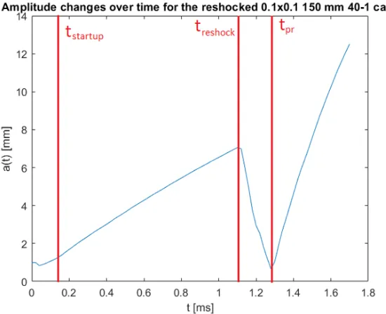
Another reference value that is used to consider the effects of the reshock, is the moment the phase reversal after reshock has completed. To compare the results of the amplitude growth after reshock, the growth after phase reversal is considered and compared, because for some cases the phase reversal takes more or less time than for others and only the growth rate after phase reversal completion is of interest. Therefore a reference timetpr is defined (where pr

RMI case. A correspondingapris defined as the amplitude attprand both can be found from

the dimensional analysis of the experiment or simulation. These moments are highlighted in an example amplitude plot, as well as the moment of reshock and can be seen in Figure 5. The growth of the amplitude, after the moment phase reversal reaches approximately 0 mm amplitude (or its lowest value), will be referred to as the post-reshock growth rate.

Figure 5: Moments of start-up completion, reshock and phase reversal completion in an amplitude plot for a reshocked RMI case

3.2.5 Multi-mode RMI

The main topic of this research is single-mode RMI. However, the implications of a multi-mode interface are also shortly discussed.

In the case of a multi-mode initial interface, non-linear processes such as mode-coupling and bubble competition, start to play a role. In the bubble competition process large bubbles are dominant over smaller bubbles, overtaking them and taking in their space. This results in a slowly growing wavelength over time. This also results in a generally faster growing MZ width. At a late time, the perturbation becomes self-similar and grows in a decaying fashion. in the self-similar stage, there is no effect of the initial conditions present, meaning this stage is independent on initial conditions.[7]

3.2.6 Current research into reshocked RMI

3.3 Goal and Hypothesis

The goal of this research is define the relationship between the initial conditions of a per-turbed interface subjected to reshock and the development of the mixing zone width after reshock. The aim is to determine if a relationship exists, and if so, to find what this relation-ship is. This is done by performing a numerical simulation of the reshocked RMI. The type of interface that will be examined is the single-mode sinusoidal perturbed interface. During the simulation process, the gaseous interface of interest must be single-mode and non-turbulent during both interaction with the initial shock, as well as interaction with the reshock. This is because the applied simulation tool, HOWD, is not suitable for examining turbulent flows, due to lack of a turbulent model.

Based on the work by Leinov et al.[8] a hypothesis is defined and stated as:

Post-reshock MZ growth is weakly dependent on the initial conditions, such as initial wavelength and amplitude.

4

Approach & Method

4.1 Research cases

In this report the research into the effects of varying reshock time and initial conditions on the growth rate of the mixing zone in reshocked RMI are examined. Several research cases are examined. They are: Recreating the simulation result by Latini et al.[6], comparing sim-ulation results to experimental data, varying the reshock time, varying initial amplitude, varying initial wave length and varying shock strength. These research cases are explained in more detail below.

4.1.1 Recreating the simulation research by Latini et al.

In order to obtain useful results the simulation method needs to be mastered before de-pendable simulations can be made. In this case it was suggested to learn to use the HOWD simulation tool by recreating the simulation results of another research. In this case the re-search by Latini et al.[6] was chosen, because it uses a 5th-order WENO method, similar to the HOWD simulation tool. The paper also clearly specifies the used simulation parameters, which makes recreating its simulation results relatively easy.

The case contains an air(acetone)/SF6shock tube situation. The simulation includes an ini-tial shock and a reshock that is reflected by the end wall of the simulated shock tube. The initial perturbance is of sinusoidal form with givena0 andk. The simulation is performed at Mach numberM = 1.21. In the paper, the results of a 5th- and a 9th-order WENO simu-lation are shown, as well as PLIF images of a comparable physical experiment.[6] The goal is to recreate the results of the 5th-order WENO simulation. In Section 5.1.1 the density im-ages are used to compare the results of the simulation. The initial conditions and simulation properties of this simulation can be found below in Table 1. In the simulation done by Latini et al. only one adiabatic exponent(gamma) is used. Although HOWD is capable of using two gamma values for air(acetone) andSF6, in the simulation also one gamma value is used, to more accurately recreate the example simulation results by Latini et al. Using one gamma instead of two can have effects on the reshock time, compared to the experimental results

Table 1: Simulation parameters as specified by Latini et al.[6]

Mach number M 1.21 [-]

Computational domain x-direction [0,Lx] [0, 780] [mm]

Computational domain y-direction [0,Ly] [0, 89] [mm]

Shock starting position x_0,shock 10 [mm]

Interface starting position x0,inter f ace 30 [mm]

Grid resolution ∆x=∆y 0.232 [mm]

Initial amplitude a0 2 [mm]

Wave length λ 59.3333 [mm]

Courant–Friedrichs–Lewy condition CFL 0.45 [-] Adiabatic exponent air(acetone) &SF6 γaa= γSF6 1.276 [-]

Molar mass air/acetone Maa 34.76 [g/mol]

The initial perturbed interface is defined as:

η(y) =a0cos(ky) (8)

where:k=2π/λis the wave number

4.1.2 Single-mode RMI simulation comparison to experiments

To validate the model, the simulation data will be compared to experimental data. To do this, a case of single-mode RMI is compared to the experimental data by Liu et al. [4]. In this paper several different amplitudes and wavelength combinations are tested. The experiment initial interface can be considered as a single-mode interface. It is created using a novel soap film technique. The results of the experiment will be compared to simulations that will be performed using the same initial conditions.

The experiment involves the impulsive accelerations of an air/SF6interface in a shock tube. As mentioned, the interface is created using a soap film technique and has a sinusoidal shape. The single-mode RMI without reshock is researched. The aim is to recreate the results of the experiment to determine the applicability of the HOWD simulation method to single-mode RMI. Four simulations were done for four differenta0/λratios. These ratios are 20/1,

40/1, 60/1 and 60/4, these different research cases will be referred to as the 20-1 case, 40-1 case, 60-40-1 case and 60-4 case, respectively. If the simulation results are found to match the experimental values, the applicability of the HOWD simulation tool is determined to be valid. Finally, if a match is found, one of the experimental cases is chosen as the base for the next experiments, from which the selected parameters will be varied.

To compare the results of the experiment to the simulation, the Schlieren density pictures will be recreated using the information of the density in the simulation. Furthermore, the amplitude of the mixing zone is measured and compared to that of the experiment.

Table 2: Simulation parameters for the simulation of the single mode RMI experiment[4]

Mach number M 1.22 [-]

Computational domain x-direction [0,Lx] [0, 200] [mm]

Computational domain y-direction [0,Ly] [0, 2λ] [mm]

Shock starting position x0,shock 10 [mm]

Interface starting position x_{0,inter f ace} 20 [mm]

Grid resolution ∆x=∆y 0.1 [mm]

Initial amplitude a0 1, 4 [mm]

Wave length λ 20, 40, 60, 80 [mm]

Courant–Friedrichs–Lewy condition CFL 0.5 [-]

Adiabatic exponent air γa 1.4 [-]

Adiabatic exponentSF6 γSF6 1.093 [-]

Molar mass air Ma 28.97 [g/mol]

4.2 Verifying mesh size

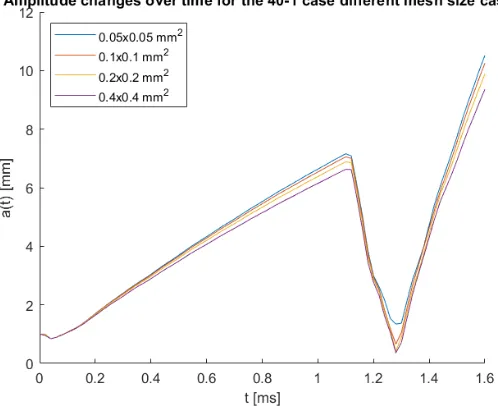
To verify that the chosen mesh size is sufficiently small and that changing the mesh size will not cause significant changes in the simulation result, several mesh sizes are compared. The results of increasingly smaller mesh size simulations are expected to show converging be-haviour for small mesh sizes. If the bebe-haviour is found to be converging and the differences with smaller mesh sizes are acceptably small, the mesh size is determined to be accurate enough.

To find a suitable mesh size, a basic reshock case (based on the single mode RMI experiments by Liu et al.[4], but introducing the reshock) is performed with different mesh sizes. the 40-1 case is examined. First off, based on the Latini et al[6]. experiment, a comparable mesh size is chosen. In this case, first an 0.1x0.1 mm mesh size is tried. After this, larger and smaller mesh sizes will be applied to the same case, to find the converging behaviour and to find the suitable mesh size. The (square) mesh sizes 0.05, 0.1, 0.2 and 0.4 mm are used. To reduce the computational time and create a suitable reshock time (so the interface is still single-mode upon reshock), the domain height is reduced to 1.5λ = 60 mm and the end wall is placed

atLx = 150 mm The resulting Schlieren images and mixing zone amplitude are examined.

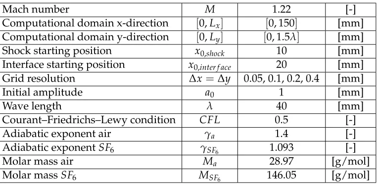
The chosen mesh size is determined by analysing the accuracy of the simulation, but also be judged depending on the time that is required to perform the simulation. A computational time that is too high can cause the project to take much longer than necessary. The exact simulation parameters are shown below in Table 3:

Table 3: Simulation parameters for the simulation of the 40-1 case with different mesh sizes

Mach number M 1.22 [-]

Computational domain x-direction [0,Lx] [0, 150] [mm]

Computational domain y-direction [0,Ly] [0, 1.5λ] [mm]

Shock starting position x0,shock 10 [mm]

Interface starting position x0,inter f ace 20 [mm]

Grid resolution ∆x =∆y 0.05, 0.1, 0.2, 0.4 [mm]

Initial amplitude a0 1 [mm]

Wave length λ 40 [mm]

Courant–Friedrichs–Lewy condition CFL 0.5 [-]

Adiabatic exponent air γa 1.4 [-]

Adiabatic exponentSF6 γSF6 1.093 [-]

Molar mass air Ma 28.97 [g/mol]

Molar massSF6 MSF6 146.05 [g/mol]

4.3 Effects of various parameters

will be the same as in Table 4. According to the results and discussion that can be found in Section 5, the 40-1 case is used as a base and a 0.1x0.1 mm2 mesh is used. The conditions of the base case can be seen below in Table 4, these values are valid for all cases mentioned below, unless a variation in parameters is mentioned in the sections below. All results are examined in both dimensional and dimensionless parameters.

Table 4: Simulation parameters for the simulation of base case

Mach number M 1.22 [-]

Computational domain x-direction [0,Lx] [0, 150] [mm]

Interface starting position x0,inter f ace 20 [mm]

Grid resolution ∆x=∆y 0.1 [mm]

Initial amplitude a0 1 [mm]

Wave length λ 40 [mm]

Courant–Friedrichs–Lewy condition CFL 0.5 [-] Adiabatic exponent air γa 1.4 [-]

Adiabatic exponentSF6 γSF6 1.093 [-]

Molar mass air Ma 28.97 [g/mol]

Molar massSF6 MSF6 146.05 [g/mol]

4.3.1 Reshock time

The first parameter that is to be examined is the reshock time (treshock). In this research, the

reshock time is defined as: the moment when the reflected shock, interacts with the per-turbed interface. This means the second time a shock interacts with the perper-turbed interface. At the moment the reshock interacts with the interface, the interface is already moving and deforming due to the initial shock interaction. At the moment of reshock interaction, the interface is in the process of developing RMI. depending on the reshock time, the interface can be single-mode or multi-mode. If the reshock time is quite late, the interface will have formed the bubbles and spikes and turbulent behaviour can be observed in the roll-up vor-tices at the edges. Since the HOWD simulation tool is not suited for observing turbulent flow, the results will be most reliable when the interface is still single-mode. With this assumption, the values of the reshock time that will be applied in the simulation, will be chosen such that the interface will show no or little turbulent behaviour at the moment of reshock.

Since reshock time is not a parameter that can be set in the simulation parameters, the reshock time is varied by varying the end wall distance. Through varying the end wall distance the moment the shock is reflected is changed and the moment the reshock interacts with the interface is also changed. Putting the end wall of the simulation area too far away can result in a multi-mode interface with turbulent mixing, which is undesirable. Therefore it is chosen to mostly focus on shorter end wall distances, keeping the interface single mode at the moment of reshock interaction. The chosen end wall distances are:Ly =175 mm, 150

mm, 100 mm and 50 mm. The exact resulting corresponding reshock times can be found after the simulation is performed.

in a different amplitude upon reshock), however in the case of the varied reshock time, the in-terface will also have developed for a different time after the initial shock. Which means that there is a variation in vorticity and pressure perturbations along the interface upon reshock. This is different from when just the initial amplitude is varied, as these cases will always have the same time to develop.

4.3.2 Wavelength

Secondly, the initial wavelength(λ) is examined and varied. Varying the initial wavelength

has a similar effect to varying the initial amplitude, as it is the ratio between these two pa-rameters that (partly) determines the development of the flow. During the simulation it is again important not to choose aλthat is too small, as it can again create the problem of

tur-bulent flow or turtur-bulent mixing occurring, which has a negative influence on the accuracy of the simulation.

For the wavelength variation, values are chosen that prevent the interface from developing into a multi-mode, turbulent interface before the reshock interacts with it. The chosen values for the experiment are: λ = 20 mm, 40 mm, 60 mm and 80 mm, while keeping the initial

amplitude ata0 =1 mm. Since the computational domain in y-direction is defined as 1.5λ,

this means that the computational domain in y-direction has to be changed for each case, to meet this requirement.

4.3.3 Initial amplitude

The case of varying initial amplitude (a0) is considered. In this case the wavelength is kept constant atλ=40 mm. The chosen values for initial amplitudes are: a0 =0.5 mm, 0.67 mm, 1 mm and 2 mm. Choosing an initial amplitude that is too large will result in the before mentioned undesirable behaviour, hence this choice of initial amplitudes.

4.4 Mach number

Finally, a research is done into varying the Mach number of the shock that is used to interact with the interface. Doing this can increase the movement speed of the interface after the intitial shock (and reshock) and this increases the development of the multi-mode turbulent interface, which is to be prevented. Therefore, a Mach number that is too high is not to be used.

each Mach number case. These things need to be determined and taken into account when processing the data after the simulation.

4.5 Research method

For this research, the mixing zone behaviour after reshock is of interest, this means that this is the moment in time that will be examined. Primarily, the growth rate of the mixing zone after reshock is examined. This is done through several methods, which are shortly discussed in this section. These are the tools that are applied to examine the interface behaviour after reshock: MZ amplitude plots, bubble and spike amplitude plots, Schlieren density pictures and videos and plots of the Fourier modes. An explanation of these tools is provided below, as well as information on how they are created.

4.5.1 MZ amplitude

The first thing to be examined are the created plots of the amplitude development of the interface. The definition of the MZ amplitude (a) was given in Section 3.2.1. To generate these plots several software tools are used. First of all, the HOWD simulation tool is used to simulate the development of the interface. Since the simulated interface contains a diffu-sive layer, the interface location is defined as:The line along the interface with the mass fraction (Mf rac) value of 0.5. The HOWD simulation results are generally displayed using Tecplot 360,

Tecplot 360 is a suite of CFD visualization and analysis tools that can handle large data sets, automate workflows, and visualize parametric results.[9] In this case, Tecplot can be used to find theMf rac = 0.5 line and export its coordinates into Matlab. A Matlab script is written

that can process the data output by Tecplot and find the amplitude of the interface.

Using Matlab, the x- and y-coordinates of the interface are analysed. The amplitude is de-fined as the difference between the maximum and minimum x-coordinate, divided by 2. The Matlab script can quickly process the files for all moments in time for which there are simula-tion results available (every 20µsa results file is created). Finally the amplitudes are plotted

against time, both in dimensional and non-dimensional form. The resulting plots can be ob-served and examined to find and investigate the MZ amplitude behaviour after reshock (and throughout the process).

4.5.2 Bubble and spike amplitude plots

The bubble (ab) and spike (as) amplitudes are found in a similar way to finding the MZ

am-plitude, however it requires more information. The bubble and spike amplitudes are defined as the distance between the edge of the bubble or spike to the neutral line of the perturbance as defined in Section 3.2.1. This neutral line is not yet known. To find it, a second simulation is carried out, using an unperturbed surface. Using Tecplot and Matlab the average(over y) location of the x-coordinate of the M_{f rac} = 0.5-line is used to determine the position of the unperturbed interface.

interface from the unperturbed interface location. When these are found, a plot can be cre-ated using Matlab, showing the development of the bubbles and spikes, after reshock, over (dimensionless) time.

4.5.3 Schlieren images

Schlieren imaging is a form of flow visualisation technique that is used to visualize flow us-ing changes in density. In experiments this is used to display the flow of gasses. it is based on the fact that rays of light bend whenever they encounter a change of density. In a Schlieren image, darkened lines occur where the density gradients are present. The Schlieren images provide information on shock waves, as well as on the interface between the two gasses.[10]

Since Schlieren imaging is a method used to display shockwaves and density changes in physical experiments, the Schlieren images are not part of the simulation results, however using the density information that the simulation provides and using Tecplot, Schlieren im-ages can be created from the simulation data. These imim-ages provide a good way to study the development of the flow and of the shockwave(s). For every recorded moment in time of the simulation cases, a Schlieren image is generated. By combining all these images, a video can be created, showing the development of the flow.

These Schlieren images are a good way to study the behaviour of the flow and its develop-ment over time. They can also be compared to the Schlieren images in the physical single-mode RMI experiments by Liu et al.[4]

4.5.4 Fourier mode analysis

Although the simulation is started with a single-mode interface, in late times, a multi-mode interface can develop as the consequence of deposited vorticity and pressure perturbations on the interface. To see the development of higher order harmonics after reshock a Fourier mode analysis is performed to view the appearance and dominance of different modes on the interface.

The Fourier mode analysis is done by performing a Fast Fourier Transform (FFT) on the known interface. The interface coordinates are once again extracted using Tecplot and Mat-lab. Afterwards a second Matlab script is used to perform the FFT. The results are plots on the different occurring Fourier modes, These plots show the different active harmonics and their development over time. Observing the higher order harmonics after reshock provides with information about the forming of a multi-mode interface after reshock and the effect of different parameters on this process. However, the interface that is researched is required not to be in a turbulent state, as this might influence the analysis of the Fourier modes. Therefore, only a short time after reshock can be analysed using this method.

4.6 HOWD simulation tool

solve the Euler equations. The high-order weighted essentially non-oscillatory (WENO) con-struction (Jiang & Shu 1996) and the double-flux algorithm are combined to ensure capturing material interfaces with high resolution and high-order accuracy.[11] The WENO method is a modern high-resolution reconstruction-evolution shock-capturing method[6]. The dis-cretization of the Euler equations is the base of the numerical algorithm, therefore the trun-cations are considered as an ’implicit nonlinear high-order numerical dissipation’, Which means that no artificial viscosity or filtering is to suppress Gibbs oscillations is required.[6]. (Gibbs oscillations occur in numerical simulations where a Fourier series is used to estimate and replicate a function. The result is an incorrectly oscillating interface/function, with os-cillations that do not die out.)

The HOWD simulation does not include a turbulent model, which means it is not suitable for modelling turbulent flows. Traditionally, turbulent flows are modelled using a simulation tool including a turbulent model like Direct Numerical Simulation(DNS) or with numer-ically dissipative shock-capturing schemes like, Monotone-Integrated Large-Eddy Simula-tions(MILES) or Implicit Large-Eddy Simulation(ILES).[6] The HOWD model can approach the DNS model by using a very fine grid, however this is very computationally inefficient and results in an extremely long computational time. Furthermore a DNS model is not suit-able for modelling shock-induced turbulent flows.

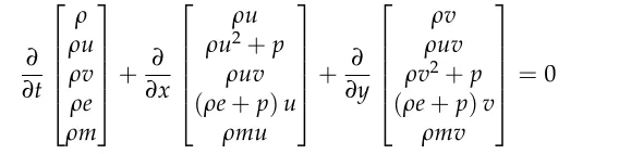
In this simulation method the Euler equations augmented by the dynamics of one fluid com-position, are adopted to model the compressible multi-component flow. This can be written as: ∂ ∂t       ρ ρu ρv ρe ρm       + ∂ ∂x       ρu ρu2+p

ρuv

(ρe+p)u ρmu       + ∂ ∂y       ρv ρuv ρv2+p

(ρe+p)v ρmv      

=0 (9)

Whereρis the density,u= #»u = (u,v)is the velocity, pis the pressure,e= (u2+v2)/2+U

is the total(kinetic+internal) energyp = ρRTis the ideal gamma law gas pressure, (Ris the

universal gas constant) andmis the mass fraction (in this case ofSF6).[6][11] The governing equations are fully conservative and hyperbolic, however straightforward employment of shock capturing schemes for multi-component flows governed by Equation 9 will generate spurious pressure oscillations at the material interface, this is why the WENO and double-flux methods are applied to prevent these oscillations.[11] Double-double-flux is a kind of method to calculate the flux at a cell edge. For two neighbouring cells with different gamma(adiabatic exponent) values, a normal flux calculation will produce nonphysical oscillation. Double-flux is a special technique to eliminate or suppress this kind of oscillation.

right, being reflected at the end and continuing its path right to left. The flow ahead of the shock is set to be stationary and the flow variables behind the incident shock are computed by the Rankine-Hugoniot relations. The boundary conditions of the upper and lower walls

Figure 6: setup of the simulation att=0 for the base case

are symmetric, while the boundary condition of the right wall is reflective (except for the case of no reshock in Sections 4.1.2 and 5.2, where an outfow condition is used) and the boundary condition of the left wall is inflow. The mesh size is set at 0.1×0.1 mm2 and is confirmed and validated in Section 5.3. Because using a Cartesian grid produces small steps along the boundary, this would cause spurious oscillations when a high-order numerical scheme (Like a 5th order WENO scheme) is applied. To correct for this issue, a technique is used to gen-erate a numerically diffusing layer. In this layer the gas concentration gradually varies from 0 to 1. In a study by Ding et al. it was varified that the employment of a diffusing layer of 3 cells can achieve high-resolution numerical solutions.[11] The initial temperatureT0 is 298.15Kand the initial pressure is 101.325 kPa. In the simulation, gas concentration factors are assumed to be 100%. Gas properties can be found in Table 5.

Table 5: Gas properties used in the simulation

Gas Molecular weight Density sound speed γ

5

Results & Discussion

In this part, the results of the research are shown and discussed. Firstly, the validation of the simulation model by recreating two research cases is discussed, this is done through compar-ison to the 5th-order WENO simulation by Latini et al.[6] and by comparcompar-ison to experiments by Liu et al.[4] Afterwards, the chosen mesh size is validated. Then the results of the main research are discussed. Schlieren images and amplitude plots are discussed for each research case. The research cases are variation in: reshock time, wave length, initial amplitude and Mach number. And the discussed results are Schlieren images, Amplitude plots of the MZ width for the whole process, as well as the process after reshock and amplitude plots for the bubble and spike amplitude. For each of these plots a dimensional and dimensionless graph is created. After this, the results of the FFT research is discussed for all cases. Finally, a comparison is made with the models mentioned in Section 3.2.3.

To prevent discussing irrelevant results and displaying too much information, the results of the simulations are displayed in appendices. Only the most relevant and interesting results are displayed in the main report.

5.1 Recreating the two research cases

Here the recreation of the simulation by Latini et al.[6] and the experiments by Liu et al.[4] is discussed. The goal is to proof the simulation tool is applied correctly and the results are applicable to a real life experiment.

5.1.1 Simulation by Latini et al.

To prove the simulation tool is applied correctly the simulation results by Latini et al.[6] are recreated. All initial conditions for this research can be found in Section 4.1.1. The paper by Latini et al. shows a physical representation of the simulation results on the form of the density plots at several points in time, as well as the amplitude plot for the process. To make a correct comparison, these figures are recreated using the HOWD simulation tool and com-pared. The results can be seen below in Figure 7.

The first thing to note (which can not be seen in this figure, but is found from the simula-tion results) is that the reshock time (i.e. the moment the reflected shock interacts with the interface) is slightly different for both cases. In the Latini et al. case the reshock occurs after 6.36 ms after initiation of the simulation, whereas the HOWD simulation shows a reshock time at 6.50 ms after simulation initiation. This difference is quite small, both reshocks occur slightly earlier than the experimental reshock time, due to the use of only one gamma value in the simulation. The difference in reshock time is the reason that the right side of Figure 7 is taken at a time corresponding to the same time after reshock, instead of the same time after simulation initiation. The second thing of note is that the HOWD simulation contains a much thicker diffusion layer along the interface. This is due to the workings of the HOWD simulation tool, which manually adds a 3 cell (see Section 4.6) diffusion layer, which might be different from the diffusion layer settings for the Latini et al. simulation. Lastly, a slight difference can be seen in the development of the interfaces. It can be concluded that the ’mushroom’ shape is more pronounced in the Latini et al. simulation. This can partly be ascribed to the thicker diffusion layer, which prevents the fine shapes that occur in the Latini et al. simulation to form.

Next, the amplitude plots for the development of the MZ amplitude are compared. The pa-per by Latini et al. only provides the dimensional plot, so this is compared to the plot created byMatlabusing the simulation results. The two plots can be found below in Figures 8.

Figure 8: Amplitude plots for the Latini et al. simulation[6](black) and the same simulation performed by the HOWD simulation tool(blue)

later and finally, during the phase reversal that occurs, the HOWD simulation shows a lower minimal amplitude than the Latini et al. simulation. This is probably caused by the way the amplitudes are determined for this plot. All with all the amplitude plots show very similar behaviour. One final thing to note is that this setup for the RMI includes multi-mode and turbulent mixing behaviour upon reshock. As mentioned in Section 4.6 the HOWD simulation tool does not include a turbulent model and is not fit for examining turbulent flows, however, the results are still very similar to this situation (and quite similar to the Latini et al. physical experiment, although both simulations show some differences with the experiment[6]). This conclusion will not be used to assume the correctness of turbulent flow simulations by HOWD.

The comparison to the Latini et al. simulation can be used to conclude that the HOWD simulation tool shows similar results to other 5th-order WENO simulations. It can also be concluded that the HOWD tool was applied correctly and is applicable to reshocked RMI situation.

5.2 Comparison to physical experiments and base case selection

Next, simulations are performed to validate the HOWD simulation tool using physical ex-periments. For this, the experiments by Liu et al.[4] were used and simulated using the in Section 4.1.2 defined conditions. The aim is to conclude that the simulation results are com-parable to physical RMI, as examined through experiments. To verify the tool, the Schlieren images from the paper by Liu et al.[4] and the recreated Schlieren images from the HOWD simulation are compared. The results of these comparisons can be found in Appendix B. These comparisons do not contain the same amount of wavelengths that are displayed, due to computational time restrictions.

In Appendix B it can be seen that the simulation results agree wel with the experimental results, with the exception of the 40-1 case, which is shown again in figure 9.

In Figure 9 it can be seen that around 1184 and 1344 ms, the experimental results have reached the phase where bubbles and spikes are created already, whereas the HOWD simu-lation result show a mostly single-mode interface for these moments in time. When observed closely, however, it is can be seen that the interface in the HOWD Schlieren image, shows the beginnings of developing the ’mushroom’ shape, especially when the edges of the spikes are observed closely. It is possible that this difference is a result of the diffusion layer that is in-serted into the initial interface. It can also be a consequence of a mesh size that is too coarse. To verify if this difference between simulation and experiment is significant, the amplitude plots are compared. Since the research mostly focuses on MZ amplitude development, it is most important that this aspect is correct for both cases. The possibility of a too coarse mesh size will be examined in Section 5.3.

Next the amplitude plots for all cases are compared. In the paper by Liu et al. a single plot is supplied that shows all dimensionless amplitude cases (as well as the cases for some mod-els) in one graph. these are compared to the created dimensionless amplitude plot for the HOWD simulation cases. These are displayed below in Figure 10.

Figure 9: Comparison of the 40-1 case of by Liu et al.[4] and the HOWD simulation

(a)

(b)

well. All experiments show approximately the same initial growth, which is reflected in the simulation results. The early time results of the simulations are nearly identical to the ones from the Liu et al. experiments. Only for the 20-1 case, it can be found that the late time behaviour differs slightly from the experimental results. The simulation data shows a higher value for the dimensionless amplitude for lateτ. This is explained by the fact that the

20-1 case reaches turbulent mixing behaviour in this late dimensional time area. Since the HOWD simulation tool does not include a turbulent model, this could explain the difference in the results. However, since the research focuses on the examination of single mode non-turbulent interfaces, this effect should not influence the research.

This leads to conclusion that the HOWD simulation tool is suitable for recreating the results of single-mode RMI experiments with decent accuracy. Noting that the tool is most suitable for examining early time behaviour that does not include turbulent mixing. Finally, from these experiments a ’base case’ is chosen in which the other parameters will be individually varied. The 40-1 case is chosen, because it has the smallest computational size with an ac-ceptably long single-mode stage, before starting to exhibit turbulent mixing behaviour. To create the base case, a reflective boundary condition is added to the end wall and the end wall position is set to 150 mm, to ensure a reshock time within the single-mode stage. Also, the computational domain height is set to 60 mm (1.5λ) to reduce computation time. For this

base case a mesh size verification is done in the next section.

5.3 Mesh size verification

Having decided on a base case, the mesh size will be verified. The goal is to determine if the behaviour of the simulation changes significantly for higher or lower mesh sizes, also if a (much) higher accuracy can be reached by using a more fine mesh size. The resulting Schlieren images of the simulation can be found in Appendix C. Here the images are shown for the time of reshock, the moment the phase reversal reaches lowest(≈0) amplitude, early time behaviour and late time behaviour. From the results in Appendix C, it can be seen that the higher mesh sizes show more perturbations along the interface for later times. This is to be expected, because a smaller mesh size allows for smaller structures to develop and these turn into turbulent vortices along the interface for later times. Another thing of note is the moment the finest (0.05x0.05) mesh size still shows perturbations along the interface for the moment the phase reversal should reach zero, this is reflected in the amplitude plot in Figure 11, where the 0.05 case does not go down as close to zero during phase reversal compared to the other cases.

Figure 11: Amplitude growth for simulations with different mesh sizes

5.4 Varying parameters

In the following section, the results of the main research are discussed. In this research, the base case is used with the simulation conditions as mentioned in Section 4.3, as well as the varied parameters mentioned in the same section. The results are displayed in in the appendices and the most important results are displayed in the main report and discussed more elaborately. The varied parameters are: reshock time, wave length, initial amplitude and initial Mach number and they are discussed in this order. The analysis includes Schlieren image analysis, MZ amplitude plots and bubble and spike amplitude plots. Each section is concluded by a short conclusion on the effect of each parameter on MZ development.

5.4.1 Reshock time

The first parameter to be tested is the reshock time. This is done through varying the end wall distance. Four cases are examined: wall distances at 50, 75, 100, 150 and 175 mm. The cor-responding reshock times for each case are 260, 480 680, 1100 and 1320 µs respectively. The Schlieren images resulting from this can be seen in Appendix D. These images show that for all cases the interface upon reshock is still single-mode which is the preferred behaviour. All different reshock times seem to show similar behaviour for the interface development after reshock. However the 50 mm case develops differently from the rest, showing no real development of spikes and bubbles or any turbulent mixing along the interface. The reason for this is, most likely, that due to the small computational domain, the boundary conditions influence the interface development through wall effect. Another explanation is that the rarefaction waves that follow the reshock very quickly for this case, influence the interface development and prevent it from developing in the same manner as the other cases. This theory is further strengthened by the amplitude plots. The Dimensionless amplitude for the whole process is shown in Figure 12.

sig-Figure 12: Dimensionless amplitude changes over time for different reshock time cases

Figure 13: MZ, spike and bubble amplitude plots

nificantly slower post-reshock growth than the other cases. Therefore it is assumed that the 50 mm case is affected by other parameters and is not taken into account for the reshock time variation comparison. Furthermore, the dimensional and dimensionless graphs (which can be found in Appendix E show no significant difference, so for further examination, the dimensionless plots are considered. The graphs for development after reshock, normalised so that all graphs start after the lowest value during phase reversal are displayed in Figure 13.

These figures show clearly that a different reshock time does not influence the early-time MZ growth rate after reshock. All amplitude growth rates, the MZ amplitude, bubble and spike amplitude show the same early-time growth rate. For late times, it can be seen that smaller reshock times result in earlier development into de non-linear stage. Finally the spike am-plitude grows much faster than the bubble amam-plitude, The bubble amam-plitude also shows oscillations for late time development, this is most likely due to the arrival of rarefaction waves to the interface.

5.4.2 Wavelength

Next, the different initial wavelength cases are considered, the tested wavelengths are: 20, 40, 60 and 80 mm. The corresponding Schlieren images for these tests can be found in Appendix F. In these Schlieren images it can be noted that the 20 mm case has already formed spikes and bubbles upon reshock and is not single-mode anymore. Furthermore, turbulent mixing is occuring along the edges of the spikes and bubbles. This means the HOWD simulation tool results are not considered reliable and the 20 mm case does not meet the single-mode requirement set in Section 4. Therefore, the 20 mm case will not be considered. Reshock occurs at the same moment for all cases (1100 µs), however not all cases go through the zero amplitude point at the same time, with the bigger amplitudes taking more time to reach the zero amplitude. Finally, the Schlieren images show that the smaller wavelengths show more and earlier development of turbulent mixing along the interface, as well as earlier develop-ment of the spikes and bubble structures. This can be seen in Figure 14 below.

Figure 14: Late time behaviour for the 80, 60 and 40 mm initial wavelength case

All amplitude plots for the different wavelength cases can be found in Appendix G. When the dimensional amplitude plots for the whole process are considered, again the reshock occurs at the same time and for the larger wavelength the phase reversal takes longer to complete. Another thing to notice is that the larger wavelengths have a slower amplitude growth after reshock than the smaller wavelengths. To verify, the post-reshock behaviour is considered and shown in Figure 15.

(a) (b)

In this figure, the difference in early time post-reshock growth rate can be quite clearly seen. The 80 mm case shows a slower growth after reshock than the other cases. However, when the dimensionless graph is considered, there is no clear difference in growth rate (except for the 20 mm case, which is multi-mode upon reshock and is therefore not considered). This means that the difference in growth rate is dependent onλand can be predicted using the

currently applied dimensionless parameters. Sincekis one of the parameters used for non-dimensionalisation andk ∼ λ, it can be concluded that a linear relationship exists between λ and post-reshock growth rate. If this assumption is correct, this means that the growth

rate can be predicted for any (single-mode upon reshock)λsituation. so from this result it

is found that thedimensionlesspost-reshock growth rate is independent of the initial wave-length parameter, for all single-mode cases. This is highly possible, because after reshock flow instability is enhanced greatly so that the flow enters a turbulent mixing state, which loses its memory of initial conditions.

To find the reason that the dimensional post-reshock growth rate is different for the different wavelength cases, the bubble and spike amplitude plots are considered. Since, the dimen-sionless amplitudes for both bubble and spike show consistent behaviour with the MZ am-plitude plot (approximately the same growth rate for all wavelength cases), the dimensional bubble and spike amplitudes are considered in Figure 16.

(a) (b)

Figure 16: (a) Spike and (b) bubble amplitude plots for different initial wavelength cases

In these results it is seen that difference in spike and bubble amplitude growth rate, for the larger amplitudes, is not as big as in the results for the 40-1 different reshock times case. Moreover, the difference in MZ amplitude growth rate is mainly created by a difference in growth rate of the spike amplitude. The spike amplitude growth rate is lower for higher ini-tial wavelengths. However for the largest iniini-tial wavelength, 80 mm, it is seen that the bubble amplitude also shows a slower development, while the other values all have the same initial growth rate. To find if this development continues for larger wavelengths, further research is required.

post-reshock MZ growth rates. This is mainly caused by a slower development of the spike amplitude, with a slower growing bubble amplitude growth rate only contributing for the largest wavelength case(80 mm). Further research into larger initial wavelengths is required to verify if this bubble amplitude behaviour is consistent for larger wavelengths. Finally, the difference in amplitude growth does not exist for the dimensionless parameters, meaning that the growth rate can be predicted for different wavelength cases in single-mode reshock scenarios.

5.4.3 Initial amplitude

The result of variation of initial amplitude on post-reshock growth rate is discussed in this section. Four different amplitudes are tested: 0.5, 0.6667, 1 and 2 mm. The Schlieren images resulting from the simulation are shown in Appendix H. These images show the devel-opment of the interface for different amplitude cases. It can be noted that the 2 mm case interface is multi-mode upon reshock and exhibits turbulent mixing behaviour. Therefore, this result is not considered for the further study. As with the different wavelength cases, the late time results show a difference in turbulence for the late time behaviour, this can be seen in Figure 17. With larger initial amplitudes contributing to more turbulent mixing occurring and earlier development into the ’mushroom’ shaped bubbles and spikes. For all cases, reshock occurs at approximately the same time and the phase reversal reaches the zero amplitude around the same time.

Figure 17: Late time behaviour for different initial amplitudes: 0.5, 0.67, 1 mm, from left to right

Next the amplitude plots are considered. These plots (among others) are shown in Appendix I. Here, it can again be seen that reshock occurs at the same time, however post-reshock growth rates differ shortly after reshock and disperse further for later times. Comparing all cases, differences in pre-reshock behaviour are noted, such as different initial amplitude growth rate(non-existent in the dimensionless amplitude plot), however the post-reshock be-haviour is considered for this research. The image shows that for smaller initial amplitudes, the post-reshock MZ growth rate is slightly smaller than for larger amplitudes.These plots give an unclear image of the dimensionless amplitude growth rate, as they are far apart. To get a clearer image of the post-reshock development, the plots are normalised to only show the post-reshock behaviour. The result can be seen in Figure 18.

(a) (b)

Figure 18: (a) Dimensional and (b) dimensionless amplitude plots for different initial ampli-tude cases, post-reshock

parameters. The dimensionless time τ is linearly dependable on the initial amplitude as,

v0 ∼ a0. This means that the effect of the variation of initial amplitude is non-linear. The effect on the post-reshock growth rate seems smaller than the effect of the wavelength. To find the reason for the slower development for smaller initial amplitudes, the bubble and spike amplitude plots are considered. the spike amplitude plots can be found in Appendix I. These show similar behaviour as the general MZ amplitude plots. The bubble amplitude plots are shown below in Figure 19.

(a) (b)

Figure 19: (a) Dimensional and (b) Dimensionless bubble amplitude plots for different initial amplitude cases, post-reshock

MZ amplitude development in the dimensional parameters is almost solely dependable on the difference in spike amplitude development, the dimensionless case shows a dependence on both bubble and spike dimensionless amplitude development.

In conclusion, a weak dependence exists between the initial amplitude and the post-reshock growth rate. Smaller initial amplitudes result in a slower post-reshock growth rate. The slower growth rate is mainly caused by a decrease in spike amplitude growth after reshock. It is also found that the effects of initial amplitude variation are also present in the system of dimensionless parameters.

5.4.4 Mach number

The final parameter to be tested is the initial Mach number of the simulation. The Mach numbers 1.1, 1.22, 1.5 and 2 were tested. The resulting Schlieren images can be found in Appendix J. unfortunately, for two of the four cases, the amplitude upon reshock is already exhibiting turbulent mixing behaviour, as can be seen below in Figure 20.

Figure 20: Schlieren images of different Mach number cases at reshock interaction with the interface, note that the pictures have been deformed to fit the page

In these pictures it can be seen that for the Mach 1.5 and Mach 2 case the interface is multi-mode and exhibits turbulent mixing behaviour, therefore the results of these simulations are not considered accurate. Furthermore, the Mach 2 case experiences reshock very close to the end wall, resulting in unwanted effects of the wall on the interface in the form of rarefaction waves and interfering boundary conditions. This can be seen more clearly in Appendix J. One other thing to note is that the attempt to keep the reshock time the same for all situa-tions is fairly successful, with only the Mach 2 case having a significant deviation.

In the following part a look is taken at the amplitude plots for the Mach 1.1 and 1.22 case. For the amplitude plots for all Mach number cases, refer to Appendix K. Although 2 results are not considered to be enough to define the any general behaviour, the results are discussed shortly nonetheless. Firstly the amplitude plots for the whole process are displayed in figure 21.

In these figures it can be seen that the initial growth rate before reshock is different. Again the figures show that reshock occurs at (approximately) the same time, however, phase reversal takes longer to complete for the lower Mach number case. This is not visible in the dimen-sionless graph, where the initial dimendimen-sionless growth rate is the same for both cases and can most likely be predicted for all single-mode cases, using the dimensionless parameters. Phase reversal takes approximately the same amount of dimensionless timeτto complete.

(a) (b)

Figure 21: (a) Dimensional and (b) dimensionless amplitude plots for different initial Mach number cases

(a) (b)

From these figures it appears that a higher initial Mach number results in a higher post-reshock growth rate. These differences are less apparent in the dimensionless plot. However, the lack of usable simulation results means it is impossible to say if the dimensionless post-reshock growth rate can is consistent in the dimensionless parameters or not.

A definite conclusion on the effect of initial Mach number on post-reshock growth rates can not be made, due to the lack of usable simulation results. However, the few usable results seem to suggest that a higher initial Mach number will result in a larger post-reshock growth rate and therefore, increased rate of mixing after reshock. It is unclear if the post-reshock growth rate is constant for the dimensionless parameters.

5.5 Results of FFT analysis

In this section, the results of the performed Fast Fourier Transfrom(FFT) on the interfaces over time are discussed. Since the FFT method only works for non-turbulent interfaces, only the early time behaviour after reshock is discussed and all cases involving a multi-mode, turbulent interface upon reshock are not considered. Also, due to a lack of usable cases, the results of the Mach number variation analysis are not considered. The goal of the FFT analysis, is to find the development of the higher order harmonics after reshock and if their behaviour is constant for the different parameters, or if certain parameters effect the higher order harmonics more than others.

The results of the FFT can be seen in large in Appendix L and also displayed below. Firstly the results of the base case are examined. The resulting figure including the first 4 harmonics is displayed in Figure 23.

Figure 23: Amplitudes of the first 4 harmonics of the interface of the 40-1 case over time

the interface, which is the same as the MZ amplitude examined in the earlier sections of the report. When Figure 23 is compared to (0.1x0.1 mm2) 40-1 case in Figure 11 almost an exact match is found, meaning the interface analysis used by the FFT Matlab program is correct and comparable to the interface analysis that has been used by the (different) Matlab script that was used so far. For the current research, only the amplitude development after reshock is considered. In Figure 23 it can be noted that after reshock, all different modes reduce to zero. After this, all modes increase slightly with the biggest increase in the second harmonic and the smallest increase in the 3rd harmonic. To see if this behaviour is consistent for the parameter variations, similar plots are created for the different (non-turbulent, single-mode) cases, shown in Figure 24.

Figure 24: Amplitudes of the first 4 harmonics of the interface for different parameter varia-tion cases over time

Most FFT results show comparable behaviour to that of the base case for the 2nd harmonic (noting the differences of the x- and y-axes), except for theλ = 80 mm case, where the 2nd

harmonic reduces to zero near the end of the plot. However, the 2nd harmonic experiences a ’hop’ in all graphs, before increasing. It is most likely that this reduction to zero is the end of the ’hop’ in the graph and that the 2nd harmonic will increase afterwards. Looking at the different wavelength cases, it can be observed that the length of this ’hop’ in the 2nd harmonic line increases for larger wavelengths, which further proves this theory. For all cases the 3rd and 4th harmonic increase only slightly after reshock. Finally, from the different amplitude cases it can be deducted that a larger initial amplitude results in a faster growth of the 2nd harmonic.