University of Warwick institutional repository: http://go.warwick.ac.uk/wrap
This paper is made available online in accordance with
publisher policies. Please scroll down to view the document
itself. Please refer to the repository record for this item and our
policy information available from the repository home page for
further information.
To see the final version of this paper please visit the publisher’s website.
Access to the published version may require a subscription.
Author(s): Yvo Pokern, Andrew M. Stuart, Eric Vanden Eijnden
Article Title: Remarks on Drift Estimation for Diffusion Processes
Year of publication: 2009
Link to published version:
http://dx.doi.org/
10.1137/070694806
REMARKS ON DRIFT ESTIMATION FOR DIFFUSION PROCESSES
YVO POKERN∗, ANDREW M. STUART†, AND ERIC VANDEN-EIJNDEN‡
Abstract. In applications such as molecular dynamics it is of interest to fit Smoluchowski and Langevin equations to data. Practitioners often achieve this by a variety of seeminglyad hoc
procedures such as fitting to the empirical measure generated by the data, and fitting to properties of auto-correlation functions. Statisticians, on the other hand, often use estimation procedures which fit diffusion processes to data by applying the maximum likelihood principle to the path-space density of the desired model equations, and through knowledge of the properties of quadratic variation. In this note we show that these procedures used by practitioners and statisticians to fit drift functions are, in fact, closely related and can be thought of as two alternative ways to regularize the (singular) likelihood function for the drift. We also present the results of numerical experiments which probe the relative efficacy of the two approaches to model identification and compare them with other methods such as the minimum distance estimator.
Key words. parameter estimation, diffusion process, nonparametric estimation, maximum likelihood principle, minimum distance estimator, reversible diffusion process, molecular dynamics, Langevin equation.
AMS subject classifications. 62M05 Markov processes: estimation 65C30 Stochastic differ-ential and integral equations
1. Introduction. In many applications (such as molecular dynamics, econo-metrics, atmospheric sciences and signal processing) it is of interest to fit a diffusion process to a time-series. The data may come from experiments, or from the numeri-cal simulation of larger and more complex models, either deterministic or stochastic. The objective of the present paper is to discuss some issues that arise when apply-ing a maximum likelihood inference method to this problem. In so doapply-ing, we will highlight some connections between this approach, favored by statisticians, and other approaches used in the physics and chemistry literature.
To introduce the maximum likelihood inference framework and some of the issues that we will discuss, it is useful to consider first the specific case when it is known that the data is consistent with an Itˆo stochastic differential equation of the form:
˙
Xt=−∇V0(Xt) +
p
2β−1W˙
t (1.1)
This equation is often referred to as the Smoluchowski or overdamped Langevin equa-tion in the chemical-physics literature. Precise statements of the observaequa-tions about this problem given here will be provided in Section 2.1. In Section 2.2 we consider gen-eral reversible diffusions and in Section 3 the (non-reversible) second order Langevin equation.
In equation (1.1),Wtis a standardd-dimensional Brownian motion inRd,β >0 is
a constant playing the role of the inverse temperature, andV0:Rd→Ris a potential which we assumeC2, bounded from below and with a growth condition at infinity to guarantee thate−βV0 is integrable. In this case, the process defined by (1.1) is ergodic with respect to the Boltzmann-Gibbs measure associated withV0 whose density is
ρ0(x) =Z−1e−βV0(x) where Z =
Z
Rd
e−βV0(x)dx. (1.2)
∗Department of Statistics, University of Warwick, Coventry CV4 7AL, England. †Mathematics Institute, University of Warwick, Coventry CV4 7AL, England. ‡Courant Institute, New York University, New York, USA.
We assume that β is known and that we wish to estimate the potential V from the data, i.e. from a sample path {Xt}t∈[0,T] for some T > 0. For the time being we assume that a continuous sample of the path is available; later on in the paper, we will also discuss the problem when Xt is sampled at discrete times. To see how the
problem of estimating V given β can be cast into a maximum likelihood inference problem, letZtsolve (1.1) forV0≡0 so that
˙
Zt=
p
2β−1W˙
t, (1.3)
and let P and Qbe the path-space measures generated on [0, T] by (1.1) and (1.3) respectively. Then these measures are absolutely continuous with Radon-Nikodym derivative
dP
dQ= exp(−T IT(X)) (1.4)
where
IT(X) = β
4T
Z T
0 |∇
V0(Xt)|2dt+ 2h∇V0(Xt), dXti, (1.5)
and h·,·i denotes the Euclidean inner product on Rd and | · | the Euclidean norm,
and the integral with respect to dXt is to be understood in the Itˆo sense. The
functionalIT(X) given by equation (1.5) is proportional to the negative logarithm of
the probability density of the path{Xt}t∈[0,T] with respect to the measure on path-space generated by (1.3). When a single path{Xt}t∈[0,T] is given, if we evaluate (1.5) with potentialV rather thanV0, this object becomes a functional ofV. This functional is the negative of the log likelihood function forV:
IT(V) = β
4T
Z T
0 |∇
V(Xt)|2dt+ 2h∇V(Xt), dXti (1.6)
Thus, it is natural to try to minimize (1.6) overV to obtain the maximum likelihood estimator (MLE) for this function. Indeed, using (1.1), (1.6) can be written as
IT(V) = β
4T
Z T
0 |∇
V(Xt)|2−2h∇V(Xt),∇V0(Xt)idt
+
√
2β
2T
Z T
0 h∇
V(Xt), dWti
(1.7)
Letting T → ∞, the stochastic integral in this expression tends to 0 almost surely (a.s.), whereas the time integral converges a.s. toward an expectation with respect to the equilibrium measure with density (1.2). In other words, as T → ∞, IT(V)
converges a.s. to the functionalI∞(V) given by
I∞(V) = β
4
Z
Rd |∇ V(x)|2
−2h∇V(x),∇V0(x)i
ρ0(x)dx (1.8)
This functional is quadratic and convex in ∇V and, by completing the square, it is clearly minimized when ∇V =∇V0, i.e. when V =V0+C where C is an arbitrary (and irrelevant) constant. Thus the MLE for−∇V0given by maximizing the limiting functional (1.8) is indeed the actual drift in (1.1).
The problem, however, is that the the data{Xt}t∈[0,T] is finite, T <∞, i.e. we are obliged to work with (1.6) and have no access to its infinite time limit (1.8). To see what problems this creates, let us first put (1.6) in a more convenient form by converting the Itˆo stochastic integral h∇V(Xt), dXti into the Stratonovich integral
using
h∇V(Xt),◦dXti=h∇V(Xt), dXti+β−1∆V(Xt)dt.
Sinceh∇V(Xt),◦dXti=dV(Xt) this gives
IT(V) = β
2T V(XT)−V(X0)
+ β 4T
Z T
0 |∇
V(Xt)|2−2β−1∆V(Xt)dt (1.9)
The time integral in (1.9) can be transformed into a configuration integral using the occupation measureµT defined such that, for any Borel setB ⊂Rd, one has
µT(B) =
1
T
Z T
0
1B(Xt)dt (1.10)
where 1B(x) is the indicator function of the set B. The measure µT is the finite
time equivalent of the equilibrium measureρ0(x)dx entering (1.8). UsingµT, we can
write (1.9) as
IT(V) = β
2T V(XT)−V(X0)
+β 4
Z
Rd |∇ V(x)|2
−2β−1∆V(x)
µT(dx). (1.11)
This expression (1.11) makes it apparent why an attempt to directly minimize this functional overV is a bad idea. When d = 1, the occupation measureµT has the
scaled local timeLx
T/T of the process{Xt}t∈[0,T] as a density, butLxT is only H¨older
continuous up to C0,1
2(R). Indeed, Lx
T has the fine-scale properties of a diffusion
process (cf. the Ray-Knight description of Brownian local times). In the appendix, we show that (1.11) evaluated withµT(dx) =w(x)dxwherew(x) is a one dimensional
Brownian motion, is not bounded from below. Whend >1,µT is singular with respect
to the Lesbegue measure since it is supported on {Xt}t∈[0,T]. ThusIT(V) must be
regularized in some way to become useful. There are at least three obvious ways to perform such a regularization.
1. The first way, which we will not discuss in this paper, is to adopt a Bayesian non-parametric approach in which a prior measure on V is introduced that is sup-ported on sufficiently regular functions only. By sampling from this measure and using the exponential of the negative of (1.6) or, equivalently, (1.11) as reweighting density, it is possible to sample the posterior distribution ofV given the data{Xt}t∈[0,T]. This
approach is discussed in [16] and we refer the reader to that paper for details.
2. A second way to regularize (1.11) is to assume a parametric form forV, e.g. as a linear combination of smooth basis functionsfi(x),
V(x, θ) =
N
X
j=1
θifi(x). (1.12)
where θ1, . . . , θN are weights. By substituting (1.12) into (1.6), one is left with a
quadratic function ofθ= (θ1, . . . , θN)∈RN
IT(θ) = β
4T
Z T
0
N
X
i=1
θi∇fi(Xt)
2
dt+ 2
N
X
i=1
θih∇fi(Xt), dXti
!
. (1.13)
For appropriate choice offi(x), this quadratic function of θ is convex and therefore
has a unique minimum ˆθwhich can be found by solving a linear algebraic system. This approach is the one often adopted in the statistics literature to identify a parametric approximation to the MLE ofV. We will refer to it as theparametric approach. Notice that it is crucial for this approach to work that the sum in (1.12) be finite, since it is this which regularizes the functional (1.6); the actual (non-parametric) MLE for
V will not exist in general.
3. A third way to regularize (1.11) is to regularize the measureµT(dx) and replace
it by ρT(x)dx, whereρT(x)>0 is a smooth probability density function. With this
substitution, (1.11) becomes
IT(V) = β
2T V(XT)−V(X0)
+ ˜IT(V) (1.14)
where
˜
IT(V) = β
4
Z
Rd |∇ V(x)|2
−2β−1∆V(x)
ρT(x)dx (1.15)
IfT is large enough, it is reasonable to neglect the first term on the right-hand side of (1.14), i.e. approximate IT(V) by ˜IT(V). To identify the minimizer of ˜IT(V),
note that ifρT(x)>0 and for potentials V such that limx→∞∇V(x)ρT(x) = 0, an
integration by parts yields
˜
IT(V) = β
4
Z
Rd |∇
V(x)|2+ 2β−1
h∇V(x),∇logρT(x)iρT(x)dx
= β 4
Z
Rd |∇
V(x) +β−1∇logρT(x)|2−β−2|∇logρT(x)|2ρT(x)dx.
(1.16)
This last expression shows that the minimizer of ˜IT(V) is unique up to a constant
and given by
ˆ
V(x) =−β−1logρ
T(x) +C′ (1.17)
where C′ is an arbitrary constant. This expression forV is the one usually adopted in the physics and chemistry literature and we will refer to it as thenon-parametric approachsince (1.16) and, hence, (1.17) involve no direct parametrization ofV. No-tice however that this approach leaves as an auxiliary problem the issue of determining
ρT(x). Thus, rather than removing the issue of parameterisation, it merely displaces
it toρT(x). This density can itself be obtained by minimization of some appropriate
functional (see (4.10) in the section on Numerics).
The calculations above show some of the issues that arise when a maximum likeli-hood inference method is applied to estimate the drift (here−∇V0(Xt)) in a diffusion
(here (1.1)). They also uncover a connection between the maximum likelihood infer-ence method often adopted by statisticians and the procedure of fitting V to some empirical equilibrium density which is used by chemists and physicists. In the re-mainder of this paper we will generalize this connection. Specifically:
1. In Section 2, we will clean up the calculations above and prove the facts that we just listed. We will also outline how these calculations could be generalised to a generic time-reversible diffusion and indicate that a connection between the maximum
likelihood inference and the procedure of fitting the drift to some empirical equilibrium density may exist in this case as well.
2. In section 3, we will generalize these conclusions to a specific non-reversible diffusion of great practical importance, namely the Langevin equation, a hypo-elliptic diffusion process found by coupling a Hamiltonian system to a heat bath via white noise and damping.
3. In section 4, we will perform a series of numerical experiments to illustrate our results and discuss a series of remaining issues: What is the influence of neglecting the boundary terms in (1.14)? What happens when the data is sampled at discrete times (in this case (1.6) and (1.9), and hence (1.6) and (1.11) are no longer equivalent)? What are the options to estimateρT(x) in (1.14)?
2. Drift inference for time-reversible processes.
2.1. Smoluchowski equation. In this section we make precise the results in the Introduction.
First we analyze some properties of the log likelihood function IT(V), written
either as in (1.6) or (1.11). We start by stating a theorem which indicates that attempting to minimize (1.11) directly may be ill-advised. We do this in the special cased= 1 and where the domain of integration is restricted to [0,1] and boundary terms are neglected, i.e. we consider the funtional:
IB(b) =
Z 1
0
b2(x)−b′(x)
µ(dx) (2.1)
forb∈H1(0,1).
Theorem 2.1. Ifµ(dx)in (2.1)is absolutely continuous with respect to Lebesgue measure with density given by a realisation of the Brownian bridge, then the functional IB(b)is almost surely not bounded below forb∈H1(0,1).
Proof. See the appendix.
While singular in the sense above whenT <∞, the log likelihood functionIT(V)
has a nice limit asT → ∞, as shown by the following:
Theorem 2.2. Assume that there exist C1, C2>0 such that for all x∈Rd
C1+hx,∇V0(x)i ≥C2|x|2
and that both V0(x)andV(x)are polynomially bounded. Then asT → ∞, the func-tionalIT(V)in (1.6) converges a.s. to the functionalI∞(V)defined in (1.8).
This theorem is a consequence of the following lemma:
Lemma 2.3. Under the assumptions of Theorem 2.2, equation (1.1) is ergodic with respect to the equilibrium measure with the density (1.2) and
lim sup
t→∞
√2β
2T
Z T
0 h∇
V(Xt), dWti= 0 a.s. (2.2)
Proof. The ergodicity follows from [14]. Theorem 5.5 of Chapter 2 in [13] implies that
lim sup
t→∞
|Xt| √logt ≤
r
2e
C2β a.s. (2.3)
LetLdenote the generator of the process (1.1). By the Itˆo formula we have
V(Xt)−V(X0) =
Z T
0
(LV)(Xt)dt+
Z T
0 h∇
V(Xt), dWti a.s. (2.4)
Now divide (2.4) byT.
1
T (V(Xt)−V(X0)) =
1
T
Z T
0
(LV)(Xt)dt+
1
T
Z T
0 h∇
V(Xt), dWti.
The bound (2.3) shows that the term 1
T(V(Xt)−V(X0)) tends to zero. Also, by
ergodicity
1
T
Z T
0
(LV) (Xt)dt→
Z
RdL
V(x)ρ0(x)dx= 0
sinceL∗ρ
0= 0. Thus, (2.2) follows.
Next we analyze the parametric log likelihood function (1.13) used in the para-metric approach. We have
Theorem 2.4. Let F ={fij} be the matrix with entries
fij =
1
T
Z T
0 h∇
fi(Xt),∇fj(Xt)idt, i, j= 1, . . . , N (2.5)
and assume that F is positive definite. Then (1.13) has a unique minimizer. In addition, this minimizer is then given by
ˆ
θ=F−1h (2.6)
wherehis the vector with components
hi=−
1
T
Z T
0 h∇
fi(Xt), dXtidt, i= 1, . . . , N. (2.7)
Furthermore, if the∇fi are polynomially bounded thenlimT→∞F exists and is almost surely invertible.
Proof. Immediate.
Finally, we analyze the properties of the approximate log likelihood function ˜
IT(V) in (1.14) used in thenon-parametric approach. An immediate consequence
of (2.3) is that the boundary term in (1.14) is negligible.
Theorem 2.5. Under the assumptions of Theorem 2.2, we have, for any ε >0, that
lim sup
t→∞
V(Xt)
tε = 0 a.s. (2.8)
The next theorem shows that the minimization problem associated with (1.15) has a unique solution as long as the density ρT in this functional satisfies some
re-quirements. To be able to state it more neatly, we introduce the spaceV as follows. For any open and bounded subsetU ⊂Rd define
V(U) =
V ∈H1(U) :
Z
U
V(x)dx= 0
Theorem 2.6. Let ρT :Rd →Rbe smooth, ρT ∈C∞(Rd). Furthermore, let U be a bounded open subset of Rd and letρT be bounded below onU: ∃ε >0,∀x∈U : ρT(x)> ε. Then the minimizer of
inf
V∈V(U)
β
4
Z
U
|∇V(x)|2−2β−1∆V(x)ρT(x)dx (2.9)
is unique and given by
ˆ
V(x) =−β−1logρT(x) +C where C=β−1
Z
U
ρ(x)dx (2.10)
The theorem can be proved using results from [4] but the proof can also be carried out by directly completing the square. The basic idea was given in the developments made in (1.16).
2.2. The generic time-reversible diffusion process. In this section, we as-sume that the data {Xt}t∈[0,T] has been generated by the following Itˆo stochastic differential equation:
˙
Xt=b0(Xt) +σ0(Xt)dWt (2.11)
where b0 : Rd → Rd is the drift coefficient, σ0 : Rd×Rd → Rd is the diffusion coefficient, and Wt is a standard d-dimensional Brownian motion. We assume that
the diffusion coefficientσ0(x) is known and satisfies
∃C >0 : hη, σ0σ0T(x)ηi ≥C|η|2 ∀x, η∈Rd (2.12) and that we wish to estimate the driftb0(x). We also assume that the process gener-ated by (2.11) is ergodic with respect to the equilibrium measure with densityρ0(x) (which we do not know a priori) and that this process is time-reversible. This last assumption means that
{Xt−T /2}t∈[−T /2,T /2] and{XT /2−t}t∈[−T /2,T /2] are equivalent in law
in the limit as T → ∞. (2.13)
The time-reversibility also implies thatb0(x),a0(x) =σ0σ0T(x) andρ0(x) are related as
0 =b0ρ0−12div(a0ρ0) (2.14)
which expresses that a time-reversible process has no probability current at equilib-rium. Note that sinceρ0is unknown to us (onlyσ0and hencea0=σ0σ0T are assumed to be available), (2.14) cannot be used a priori to determine b0. Nevertheless, the non-parametric approach would be to simply approximate ρ0 in (2.14) by some empirical density ρT and thereby obtain an estimate for b. Next we show that this
approach is closely related to the parametric approach in that both approaches correspond to minimizing a different regularization of the likelihood functional forb0. Proceeding as in the Introduction, we can derive the negative of the log likelihood functional for the unknown drift b given the data {Xt}t∈[0.t]. Up to an irrelevant
constant, this functional is
IT(b) =
1
T
Z T
0
|b(Xt)|2a0(Xt)dt−2hb(Xt), dXtia0(Xt)
(2.15)
where we introduced the following inner product and norm on the tangent space at
x∈Rd:
hη, ξia0(x)=hη, a0−1(x)ξi ∀η, ξ∈Rd,
|η|2
a0(x)=hη, ηia0(x) ∀η∈R
d. (2.16)
This inner product and the norm are well defined since a0(x) is invertible at every
x∈Rd by assumption (2.12).
As in (1.6), the log likelihood function (2.15) forbis unbounded below in general if the data is finite, T < ∞. We can however proceed as for the Smoluchowski equation (1.1) along the following lines:
1. If we letT → ∞, (2.15) tends to a functional whose unique minimizer isb0. 2. If we parametrizebby the following form suggested by (2.14)
b(x) = 12diva0(x)−1
2a0(x)∇V(x, θ) (2.17) with V(x, θ) as in (1.12) (thus V(x, θ) is approximating−logρ0), (2.15) becomes a quadratic and convex function for θ = (θ1, . . . , θN) whose unique minimizer can be
determined by solving a linear algebraic problem. This is theparametric approach.
3. There is an alternative way to regularize (2.15) which involves transform-ing the time integral in (2.15) into an expectation with respect to the occupation measure (1.10), and approximatingµT(dx) byρT(x)dx whereρT(x) is some smooth
density. Then the minimizer of this regularized log likelihood function is unique and related to ρT in the same way as b0 is related to ρ0 in (2.14). This is the non-parametric approach.
Let us analyze in more detail the statements made in these three points. The statement made in point 1 is a simple consequence of using (2.11) to re-write (2.15) as
IT(b) =
1
T
Z T
0
|b(Xt)|2a0(Xt)−2hb(Xt), b0(Xt)ia0(Xt)
dt
−T2
Z T
0 h
b(Xt), σ0(Xt)dWtia0(Xt)
(2.18)
In the limit as T → ∞, we would expect, by exploiting time-reversibility, that the stochastic integral converges a.s. to zero; this is exactly what happens for the Smolu-chowski equation (see Lemma 2.3). By ergodicity, the first integral converges a.s. towards an expectation with respect to the equilibrium distribution with densityρ0. Thus,IT(b) is expected to converge almost surely towards the functionalI∞(b) given by
I∞(b) =
Z
Rd
|b(x)|2a0(x)−2hb(x), b0(x)ia0(x)
ρ0(x)dx (2.19)
If ρ0(x) > 0, completing the square shows that the minimizer of this functional is unique and given by b(x) = b0(x), as needed. Of course, (2.19) is unavailable in practice since the data is finite.
Consider now the statement made in point 2. If we insert (2.17) into (2.15) and neglect all the irrelevant terms independent of θ, as well as an overall multiplicative constant, we arrive at
where ¯F ={f¯ij}is the matrix with entries
¯
fij =
1
T
Z T
0 h∇
fi(Xt), a0(Xt)∇fj(Xt)idt, i, j= 1, . . . , N (2.21)
and ¯his the vector with components
¯
hi= 1 T
Z T
0
(h∇fi(Xt),diva0(Xt)idt−2h∇fi(Xt), dXti), i= 1, . . . , N (2.22)
This is a quadratic function inθwhich is strictly convexiff the matrixF is positive definite. If this is the case, (2.20) has a unique minimizer given by
θ= ¯F−1¯h (2.23)
These results are the equivalent for (2.11) of Theorem 2.4 for the Smoluchowski equa-tion (1.1). Note that these results remain true even if the process defined by (2.11) is not time-reversible, since (2.20) remains the parametric approximation via (2.17) of the negative log likelihood function for b irrespective of whether the process is time-reversible or not.
To establish the statements made in point 3 above, we will use the following relation between the Itˆo integral in (2.15) and the corresponding Stratonovich integral
Z T
0 h
b(Xt), dXtia0(Xt)=
Z T
0 h
b(Xt),◦dXtia0(Xt)
+1 2
Z T
0 h
b(Xt),diva0(Xt)ia0(Xt)−divb(Xt)
dt
(2.24)
Using this relation as well as the occupation measureµT of the process{Xt}t∈[0,T],
(2.15) can be written at
IT(b) =
Z
Rd
|b(x)|2
a0(x)+ divb(x)− hb(x),diva0(x)ia0(x)
µT(dx)
−T2
Z T
0 h
b(Xt),◦dXtia0(Xt)
(2.25)
The stochastic integral in this expression is a correction term which we expect to vanish in the limit asT → ∞, i.e. we would expect We have
lim sup
T→∞ 1
T
Z T
0 h
b(Xt),◦dXtia0(Xt)= 0 a.s. (2.26)
Thus, if we assume that T is large enough so that we can neglect the stochastic integral term in (2.25) and we approximate the occupation measureµT(x) byρT(x)dx
whereρT(x) is a smooth density with bounded support, we can approximate the log
likelihood function (2.25) by
˜
IT(b) =
Z
Rd
|b(x)|2
a0(x)+ divb(x)− hb(x),diva0(x)ia0(x)
ρT(x)dx (2.27)
This functional is the equivalent for (2.11) of the expression (1.15) for the Smolu-chowski equation (1.1). Given the smoothness of the density we can perform the following partial integration:
˜
IT(b) =
Z
Rd
|b(x)|2a0(x)ρT(x)−b(x)· ∇ρT(x)− hb(x),diva0(x)ia0(x)ρT(x)
dx,
(2.28) where the boundary terms vanish since ρT(·) has bounded support. This functional
has much nicer properties than the originalIT(b) in (2.15) as shown by the following
result:
Theorem 2.7. Let U be a bounded open subset of Rd and assume that ρT ∈ C∞(U) is bounded below on U:
∃ε > 0 : ρT(x) > ε ∀x ∈U. Furthermore, assume that a0(·) ∈ C∞(U) is positive definite symmetric everywhere on U and its lowest eigenvalue is bounded below: infx∈Uλmin(a0(x))>0. Then for the functional
˜ ˜
IT(b) =
Z
U
|b(x)|2
a0(x)ρT(x)−b(x)· ∇ρT(x)− hb(x),diva0(x)ia0(x)ρT(x)
dx
(2.29)
the minimizer of
inf
b∈L2(U) ˜ ˜
IT(b)
is unique and given by
˜
b=1
2div(a0ρT)/ρT (x∈U) (2.30)
Proof. Rewrite the functional ˜I˜ introducing an extra factor ofρT and a0 in the middle term to recognise it as a quadratic form inb:
˜˜
I(b) =
Z
U
|b(x)|2a0(x)− hb(x), a0(x)∇ρT(x)
ρT(x) ia0(x)− h
b(x),diva0(x)ia0(x)
ρT(x)dx.
Now complete the square to obtain
˜˜
I(b) =
Z
U
b(x)−a0(x) 2
∇ρT(x) ρT(x) −
1
2diva0(x)
2
a0(x)
−
a0(x) 2
∇ρT(x) ρT(x) −
1
2diva0(x)
2
a0(x)
ρT(x)dx
SinceρT(·) is strictly positive onU, this functional is minimised when
0 =b−a0(2x)∇ρρT
T −
1
2diva0. (x∈U) (2.31)
This is an algebraic equation forbwhose solution is (2.30).
Relation (2.30) is the equivalent of (1.17) for a generic time-reversible process and shows how thenon-parametric approachof deducing the drift coefficient from the equilibrium density and the diffusion coefficient can be generalized to this case.
An interesting consequence of the calculations above is that the time-ordering of the data is not very relevant for time-reversible processes. This is clear for the non-parametric approach based on (2.27) and leading to (2.30) in which only the empirical density ρT(x) plays a role. Similarly, we expect that time-ordering plays
only a small role in the parametric approach based on regularizing the maximum likelihood function leading to (2.20) via parametrization of the driftb. This conjecture will be verified in the numerical experiments of section 4.
3. Non-reversible processes: the Langevin equation. The calculations in section 2 rely heavily on the property that the process is time-reversible. In particular, for a non-reversible process, we would not expect 2.26 to hold in general, hence we will not be able to approximate the log likelihood function by (2.27) (the contribution from the stochastic integral term in (2.25) is missing). Another way to look at the problem is to realize that, for a non-reversible process, relation (2.14) is replaced by
j0(x) =b0ρ0−12div(a0ρ0) (3.1)
where j0(x) is a divergence-free vector field accounting for the non-zero equilibrium probability current of the non-reversible process. Equation (3.1) implies that it is not straightforward to generalize thenon-parametric approach to non-reversible processes since, on top of the diffusion tensor a0 and the equilibrium densityρ0 (or some approximations thereof), we need an approximation of the currentj0 to deduce the drift b0. This approximation of j0 will not be available in general. Despite all this, in this section we show that thenon-parametric approachcan be generalized to a specific type of non-reversible processes which frequently arises in applications, and that this approach is again closely connected to theparametric approach for these processes. The specific type of non-reversible processes are those governed by the Langevin equation:
¨
Qt+β0D0Q˙t+∇V0(Qt) =
p
2D0W˙t (3.2)
whereβ0is the inverse temperature,D0is the diffusivity andWtis a standard
Brow-nian motion. (Thus the friction coefficientγ is related toβ0 andD0 via the Einstein relation: D0=γ/β0.) We assume thatD0is known and we wish to find the potential
V0and the inverse temperatureβ0.
If we setPt= ˙Qt(Qtis referred to as position,Ptas momentum) then from (3.2)
we obtain the following system of equations:
(
˙
Qt=Pt,
˙
Pt=−β0D0Pt− ∇V0(Qt) +√2D0W˙t.
(3.3)
Note that since the noise only enters the equation for Pt, (3.3) does not define an
elliptic diffusion; it is, however, hypo-elliptic, see [14]. If one assumes thatV0satisfies the assumptions in Theorem 2.2, the process generated by (3.3) is ergodic with respect to the equilibrium distribution with density
̺0(q, p) =ρ0(q)g0(p) (3.4)
where
ρ0(q) =Z−1e−β0V0(q), g0(q) = (2πβ0)−d/2e− 1 2β0|p|
2
(3.5)
Note in particular that the equilibrium distribution is Gaussian in the momentum coordinate.
The Radon-Nikodym derivative of the measure on path-space for (3.3) with re-spect to the measure generated by
˙
Pt=
p
2D0W˙t. (3.6)
is given by
exp− T 2D0
IT(Q, P)
(3.7)
Here
IT(Q, P) =
1 2T
Z T
0 |
β0D0Pt+∇V0(Qt)|2dt+ 2hβ0D0Pt+∇V0(Qt), dPti
(3.8)
where it is understood that Qt andPt are related as ˙Qt=Ptas in (3.3). For fixed
data{Qt, Pt}t∈[0,T], we may evaluate (3.8) atV andβ different fromV0andβ0. The resulting functional is then the negative of the log likelihood function forV andβ:
IT(V, β) =
1 2T
Z T
0 |
βD0Pt+∇V(Qt)|2dt+ 2hβD0Pt+∇V(Qt), dPti (3.9)
As in the Smoluchowski case, the log likelihood function (3.9) must be regularized to be useful. The simplest way is to parametrizeV(q) as in (1.12), in which case (3.9) reduces to a function ofβandθ= (θ1, . . . , θN) which can then be minimized over these
parameters. This is theparametric approach. Next we investigate another type of regularization of (3.9) leading to the equivalent of thenon-parametric approach.
We begin by making a few transformations on (3.9). First, notice that an inte-gration by parts using the Itˆo formula and ˙Qt=Ptshows that
Z T
0 h∇
V(Qt), dPti=−
Z T
0 h
Pt,∇∇V(Qt)Ptidt+h∇V(Qt), Pti T
0
Z T
0 h
Pt, dPti=
1 2
|Pt|2 T
0 −dD0T.
Thus
IT(V, β) =
1
T
h
βD0|Pt|2+h∇V(Qt), Pti
iT
0
−dD02β+ 1 2T
Z T
0 |
βD0Pt+∇V(Qt)|2−2hPt,∇∇V(q)Ptidt
(3.10)
Under suitable conditions on the potentials V0 and V, the boundary contributions from the two integrations by parts converge almost surely to zero asT → ∞as made precise in the following lemma:
Lemma 3.1. Assume that ∃Ci>0i= 1, . . . ,5, where C1<1 andm∈Z+ such
that:
• 1
2h∇V0(q), qi ≥C1V0(q) +C2|q| 2
−C3 ∀q∈Rd;
• 0≤ |∇V(q)| ≤C4
1 +|q|2m−1
∀q∈Rd • 0≤ |∇V0(q)| ≤C51 +|q|2m−1 ∀q∈Rd.
Then there is aC >0 such that:
lim sup
t→∞
|Pt|2+|Qt|2
logt ≤C a.s.
and
lim sup
t→∞
|h∇V(Qt), Pti|+|Pt|2
t = 0 a.s.
Proof. LetH(q, p) denote the following perturbed Hamiltonian:
H(q, p) = 1 2|p|
2+V(q) +D
0β0hp, qi+D02β02|q|2+ 1.
Then
H(q, p)≥1 + 1 8|p|
2+D02β20 3 |q|
2.
The arguments in Section 3 of [14] show that there existξ6, ξ7, ξ8, ξ9>0 such that:
LH ≤ξ6−ξ7H
and
∇H,
0
√ D0
2
≤ξ8[|p|+|q|]2≤ξ9H(q, p).
Thus, applying the Itˆo formula toeξ7tH(q(t), p(t)) and use of arguments similar to those in Theorem 5.5 of Chapter 2 in [13], but applied toH(q, p) instead of|p|2+
|q|2, give the first result. The second result follows since∇V(q) is assumed polynomially bounded.
The ergodicity of the process together with the lemma imply that as T → ∞ IT(V, β) converges a.s. to the functionalI∞(V, β) given by
I∞(V, β) =−dD02β+1 2
Z
Rd×Rd
|βD0p+∇V(q)|2−2hp,∇∇V(q)pi̺0(q, p)dqdp
(3.11) Using the fact that̺0(q, p) is a product of two densities, ̺0(q, p) =ρ0(q)g0(p), and that g0(p) is Gaussian, the integral over the momentum in (3.11) can be performed explicitly. The result can be written as
I∞(V, β) = 1 2
Z
Rd
|∇V(q))|2
−2β0−1∆V(q)
ρ0(q)dq+dD02 12β2/β0−β (3.12)
The integral on the right-hand side is, up to an irrelevant constant, the same as the one in (1.15) and it is the only term involvingV. As a result, the minimum of (3.12) overV is reached whenV =V0+C, whereC is an arbitrary constant. Similarly, the last term in (3.12) is minimized whenβ =β0. Thus we conclude that, in the limit as T → ∞, the log likelihood function forV0 andβ0 has these parameters as unique maximizers.
WhenT is finite, however, we need to proceed differently. First, we can replace the time integral in (3.10) by an expectation with respect to the occupation measure of the process{Qt, Pt}t∈[0,T]:
IT(V, β) = 1 T
h
βD0|Pt|2+h∇V(Qt), Pti
iT
0
−dD02β+ 1 2
Z
Rd×Rd |
βD0p+∇V(q)|2−2hp,∇∇V(q)piµT(dq, dp)
(3.13)
Assuming thatT is large enough so that we can neglect the boundary terms in (3.10) we are left with the terms on the second line in (3.13). To regularize them, we must regularizeµT(dq, dp) by some̺T(q, p)dqdp. Consistent with (3.4), we assume that the
empirical density̺T(q, p) factorizes as̺T(q, p) =ρT(q)gT(p), whereρT(q) andgT(p)
are densities which can be estimated separately by splitting the data into{Qt}t∈[0,T] and{Pt}t∈[0,T]. Consistent with (3.5), we can further assume thatgT(p) is a Gaussian
density of the form
gT(p) = (2πβT)−d/2e−
1 2βT|p|
2
(3.14)
whereβT >0 is a parameter which can be estimated from the data as
βT−1= 1
dT
Z T
0 |
Pt|2dt. (3.15)
Substituting̺T(q, p)dqdpforµT(dq, dp) in the integral term in (3.13) and using (3.14),
the integral over the momentum can be performed explicitly. This gives the following approximation for the terms on the second line in (3.13):
1 2
Z
Rd
|∇V(q))|2
−2βT−1∆V(q)ρT(q)dq+dD02 12β2/βT −β (3.16)
This functional is similar to (3.11), except that it involves the empiricalρT and βT
instead of the actualρ0 andβ0. The following theorem is thus analogous to Theorem 2.6.
Theorem 3.2. Let U ⊂Rd be open and bounded. Suppose that ρT is bounded below onU, i.e. ∃ε >0∀x∈U : ρT(x)> εholds. Assume furthermore thatβT >0. Then the functional
˜˜
Ih(V, β) =1
2
Z
U |∇ V(q)|2
−2βT−1∆V(q)
ρT(q)dq+dD2o
1 2β
2/β
T −β
(3.17)
has a unique minizer(V, β)in H¯1(U)
×R, where the bar denotes functions of mean zero. This minimizer is given by
ˆ
V =−βT−1logρT(x) +C, βˆ=βT, (3.18)
where the constant C is such as to ensure that Vˆ has mean zero.
Proof. First establish that ˆβ =βT which is straightforward as β only occurs in
the second term. The rest of the proof proceeds analogously to Theorem 2.6. Thus, thenon-parametric approachcan be generalized to the Langevin equa-tion and leads to the fitting ofV to the empirical measure, similarly to what we found in the case of the Smoluchowski equation. Furthermore, the inverse temperatureβ is estimated from the variance of the momentum in the empirical measure.
4. Numerical Experiments.
4.1. Setup. In this section we perform a series of numerical experiments on a simple model system to illustrate the results obtained in the previous sections, in particular the relationship between the practitioners’ and statisticians’ approach to drift estimation. These experiments will also allow us to investigate two issues that we have left open so far. The first is what is the impact in theparametric approach of having a data set sampled at discrete points in time rather than continuously? The second issue is how to obtain the approximate densityρT(x) needed in the
non-parametric approach. The model system we will investigate is the one-dimensional diffusion
˙
Xt=−Xt3+
3 2Xt+
3
2W˙t, X0= 0. (4.1)
This equation is a special case of the Smoluchowski equation (1.1) with
V0(x) = 1 4x
4
−34x2 (4.2)
and β = 8/9. To generate the data, we integrate (4.1) using the Euler-Maruyama scheme with time-step ∆t forNT =⌊T /∆t⌋steps, i.e. using
X(j+1)∆t=Xj∆t−Xj3∆t∆t+
3
2Xj∆t∆t+ 3 2
√
∆t ξj, j= 0, . . . , NT−1, (4.3)
with X0 = 0 and where {ξj}j=0,...,NT−1 are independent Gaussian variables with
mean 0 and variance 1. The value of ∆tandT will be varied to measure the impact of these parameters. The Euler-Maruyama scheme produces a discrete time sample
{Xj∆t}j=0,...,NT which we will use as data. For simplicity, we will denote this data
set as{Xj}j=0,...,NT in the sequel.
In theparametric approachwe use the following polynomial representation of the forceb0(x) =−V′
0(x) =−x3+32x:
b(x, θ) = 3
X
i=0
θixi. (4.4)
Equivalently, this means that we parametrize the potentialV0(x) as
V(x, θ) = 3
X
i=0
θixi+1
i+ 1 . (4.5)
Based on this parametrization, and consistent with the time-discretization used in (4.3), we adopt the following discretized version of the log likelihood function (1.13)
IT(θ) =
1
T N
X
j=0
|b(Xj, θ)|2∆t−2b(Xj, θ) (Xj+1−Xj)
. (4.6)
The minimization of (4.6) gives rise to a linear algebraic system forθ = (θ0, . . . , θ3) which is easy to solve (the solution is similar to (2.23) in the continuously-sampled case). We refer to this solution as the MLE ˆθ.
In thenon-parametric approachthe main issue is the evaluation of the empir-ical densityρT(x) in (1.15) and (1.17). To obtain results that can be easily compared
with those of theparametric approach we will parametrizeρT as
ρT(x, θ) =Z−1(θ)e−βV(x,θ) where Z(θ) =
Z
R
e−βV(x,θ)dx (4.7)
andβ = 8/9 is given. To then determineρT(x, θ), we test and compare three different
methods. The first method is based on estimating a discretization of the empirical density obtained by a standard histogram method using an even number K of bins centered at ck = 8k/K for k =−K/2, . . . , K/2. The bins are spaced equidistantly
and the small number of samples outside [−4,4] are discarded. Denoting by ˆρk this
empirical density, we then obtainθ= (θ0, . . . , θ3) by minimizing
K/2
X
k=−K/2
|log ˆρk+βV(ck, θ)|2 (4.8)
This objective function is the discrete analog of theL2norm of the difference between
−βV(x, θ) and the log of a (putative) continuous approximation of the empirical density ρk. Note that this is a straightforward least squares problem of dimension K, so this is easily solved by standard methods. We refer to optimising (4.8) as the practitioners’ method, and call ˆθ optimising (4.8) the PME.
For the second method, note that in one-dimension, the occupation measureµT
has the scaled local timeLT(x)/T as density, so one can search the minimizer of
Z
R|
ρT(x, θ)−LT(x)/T|2dx (4.9)
which measures theL2distance betweenρ
T(x, θ) and the scaled local timeLT(x)/T.
To adapt this to time-discrete observations, it is possible to expand the square and then approximate the local time as
LT = T NT
NT
X
j=0
δXj.
This results in estimation via minimizing the following objective function overθ:
Z
R
ρ2
T(x, θ)dx−
2
T NT
X
j=0
ρT(Xj, θ) (4.10)
The third method is based on a coarsened version of (4.10) in which we use ˆρk to
replace (4.10) by
K
X
k=−K
ρ2T(ck, θ)−2ρT(ck, θ)ˆρk (4.11)
Minimizing (4.11) is slightly less accurate than minimizing (4.10), but it is computa-tionally less expensive if the number of bins is significantly smaller than the number of data points in the time-series,K≪NT. The computational cost involved in
mini-mizing (4.10) compells us to use (4.11), but we study its behaviour for several choices
of K, the number of bins in the histogram. To optimise (4.11) we use steepest de-scent together with a line search strategy and refer to the optimal ˆθas the minimum distance estimator (MDE).
More generally, using a histogram as a means of summarising the data not only smoothes the empirical density but also makes optimisation easier. In the case of the estimator (4.8), it is even unclear how this estimator could be used with the unsmoothed discrete time empirical density. Various alternative ways of obtaining a smoothed empirical density ˆρfrom the discrete time observations Xj are
conceiv-able. Established methods include kernel density estimators and even nonparametric density estimation.
4.2. Connections via Correlation. In order to establish that the link between the MLE (obtained from (4.6)) and the PME (obtained form (4.8) persists for dis-cretely observed data, we wish to study the stochastic dependency between the PME and the MLE understood as random variables.
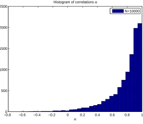
Having verified that asymptotic unbiasedness and a suitable decay of variance are indeed observed for our implementation of these estimators, we consider that these results are standard at least for the MLE, so that we do not show them here in detail. Since applied interest resides in the invariant density and the empirical measure, it seems interesting to first compare MLE and density-based estimators at the level of densities. To do this, we perform numerical simulations usingK= 50 bins for a final time ofT = 100 (and ∆t = 0.01) and compute the invariant densityρ(ˆθ,·) induced by MLE estimates ˆθ of{θi}3i=0. A typical case is shown in Figure 4.1 and repeated experiments computing the bin-wise correlation of deviations from the true invariant densityρ(whose evaluation atck we denote byρk=ρ(ck)), namely
α=
PK/2
k=−K/2(ˆρk−ρk)·
ρ(ˆθ, ck)−ρk
q
PK/2
k=−K/2(ˆρk−ρk) 2
·
r
PK/2
k=−K/2
ρ(ˆθ, ck)−ρk
2
,
show high correlations as visible in the histogram in Figure 4.2. An MDE or PME that now attempts to fit the empirical density ˆρ or its logarithm using some least squares method would hence be expected to yield drift parameter estimates ˆθwhose deviations fromθ are correlated with the MLE estimates’ deviations.
To investigate whether this is so, it is useful to note the experimental observation that all three estimators display an approximately Gaussian distribution. We use the final time T = 160 and the timestep ∆t = 0.002 and MDE and PME each use K = 50 bins throughout. We evaluate N = 1000 realisations each of MDE, MLE and PME to produce estimates of{θ(3k)}N
k=1 ofθ3. We then standardise these estimates subtracting the mean and dividing by the standard error. Histograms and Quantile-Quantile-Plots of these parameter estimates are given in Figures 4.5, 4.3 and 4.4 respectively. Furthermore, we apply a Kolmogorov-Smirnov test of normality and report the obtained p-values in these Figures. In all three cases, the observed p-value is above p= 0.88 so that the observed evidence against normality using the Kolmogorov-Smirnov test statistic is considered very weak. It should be pointed out that for smaller final times, the distribution of parameter estimates does not approximate a Gaussian as closely as this; theorems on (local) asymptotic normality that can be found for the MLE and MDE in continuous time e.g. in [11] only suggest normality for large final times.
−40 −3 −2 −1 0 1 2 3 4 0.05
0.1 0.15 0.2 0.25 0.3 0.35
x
ρ
(x)
Probability Density Functions for one Samplepath
True density
[image:19.595.109.393.110.344.2]Empirically observed density MLE induced density
Fig. 4.1.Densities from one Particular Samplepath
−0.80 −0.6 −0.4 −0.2 0 0.2 0.4 0.6 0.8 1 500
1000 1500 2000 2500
Histogram of correlations α
α
N=10000
Fig. 4.2. Correlation coefficientsαfor deviations of MLE-induced and empirical densities from the invariant density
[image:19.595.108.403.395.651.2]−30 −2 −1 0 1 2 3 4 10
20 30 40 50 60 70
Standardised MLE
Frequency
Histogram of Standardised MLE
−4 −3 −2 −1 0 1 2 3 4
−4 −3 −2 −1 0 1 2 3 4
Standard Normal Quantiles
Quantiles of standardised MLE
QQ Plot of standardised MLE versus Standard Normal
[image:20.595.114.409.105.263.2]N=1000, KS test: p−value=0.94725
Fig. 4.3.Test of Normality for the MLE
−4 −3 −2 −1 0 1 2 3 4
0 10 20 30 40 50 60 70
Standardised PM
Frequency
Histogram of Standardised PM
−4 −3 −2 −1 0 1 2 3 4
−4 −3 −2 −1 0 1 2 3 4
Standard Normal Quantiles
Quantiles of standardised PM
QQ Plot of standardised PM versus Standard Normal
[image:20.595.112.410.304.464.2]N=1000, KS test: p−value=0.9881
Fig. 4.4.Test of Normality for the PME
−4 −3 −2 −1 0 1 2 3 4
0 10 20 30 40 50 60 70
Standardised MDE
Frequency
Histogram of Standardised MDE
−4 −3 −2 −1 0 1 2 3 4
−4 −3 −2 −1 0 1 2 3 4
Standard Normal Quantiles
Quantiles of standardised MDE
QQ Plot of standardised MDE versus Standard Normal
N=1000, KS test: p−value=0.88232
Fig. 4.5.Test of Normality for the MDE
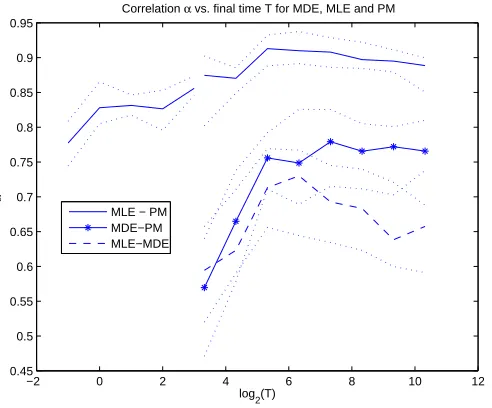
[image:20.595.112.410.507.664.2]−2 0 2 4 6 8 10 12 0.45
0.5 0.55 0.6 0.65 0.7 0.75 0.8 0.85 0.9 0.95
log 2(T)
α
Correlation α vs. final time T for MDE, MLE and PM
[image:21.595.133.379.101.305.2]MLE − PM MDE−PM MLE−MDE
Fig. 4.6.Correlations of drift parameter deviations for MDE, PME and MLE
The dotted lines indicate 33% quantile bands.
It is now appropriate to study correlations as a measure of independence, so we consider the deviations of the three estimators ofθ3from their respective means as a function of final time. Plotting their averaged correlations over at leastNav = 1000
realisations each as a function of final timeT yields the plot in Figure 4.6. It seems that the maximal obtainable correlation coefficient for is around 0.9 for the MLE-PM pair. As would be expected from the analytical link of these estimators, a decline of correlation is observed as the final timeT is decreased.
Consulting Figure 4.7, it can be seen that the number of bins has only a small influence on the observed correlation of the correlation between MLE and PME es-timates. We view this as an indication that other smoothing methods to arrive at ˆρ
would not yield significantly lower correlations.
4.3. Influence of Boundary Conditions at FiniteT. The approximation of ignoring boundary terms in going from (1.14) to (1.15) is good in the limit of large final times, as was shown in Theorem 2.5. In this subsection, we will briefly sketch the influence of ignoring these boundary terms for finite, even small final times. To do this most easily, we introduce a variant of the maximum likelihood estimator (abbreviated to MLE2) obtained by minimizing the following objective function:
IT(2)[θ] = N
X
j=0
|b(Xj, θ)|2∆t+σ2b′(Xj, θ)∆t
. (4.12)
Note that this is similar to a discretisation of (2.22) but after having performed a partial integration in the spirit of (2.24) to remove the stochastic integral and neglecting the boundary terms arising from integrating up the resulting Stratonovich integral (whereas the MLE would have been attained by discretising straight away, not performing any partial integrations). It should be compared withIT[θ] in (4.6).
In fact, the deviation of the correlation between MLE2 and MLE from 1 should indicate the influence of the initial-condition (and final value) related term on the
2 3 4 5 6 7 8 9 0.7
0.75 0.8 0.85 0.9 0.95
log 2(T)
α
PM−MLE correlations versus final time
[image:22.595.131.376.101.304.2]K=25 Bins K=50 Bins K=100 Bins
Fig. 4.7.Correlations of drift parameter deviations for MLE and PME
The dotted lines indicate 33% quantile bands.
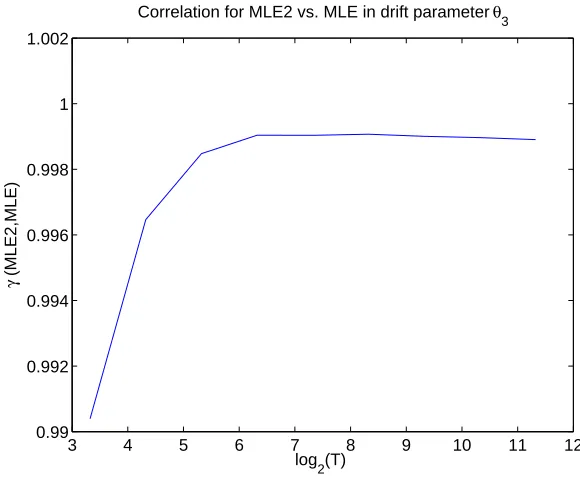
3 4 5 6 7 8 9 10 11 12
0.99 0.992 0.994 0.996 0.998 1 1.002
log2(T)
γ
(MLE2,MLE)
Correlation for MLE2 vs. MLE in drift parameter θ3
Fig. 4.8.Correlations of drift parameter deviations forA˜vs. MLE
parameter estimates. Using a similar experimental setup (with ∆t = 0.0002 this time), we compute the correlation of the MLE2 estimate and the MLE which results in Figure 4.8.
The remarkably high degree of correlation indicates that the first term which is of orderO(1
[image:22.595.101.391.350.589.2]however, decline for small final times and the onset of this decline aroundT = 10 is compatible with the decline of correlation observed in Figure 4.6.
5. Conclusions and Future Work. By analyzing different procedures to reg-ularize the likelihood function for the drift of a diffusion, we have highlighted some links between the maximum likelihood principle used widely in the statistical litera-ture, and the practitioners’ estimator based on fitting the logarithm of the empirical measure to the drift. These links have been further substantiated through selected numerical examples. In the special case of gradient diffusions these estimators are even more closely linked as their deviations from the mean value satisfy the same statistics to leading order.
At first glance the minimum distance estimator seems to be close to the non-parametric approach, but our analysis shows that the link between theparametric approachand thenon-parametric approachis far closer.
This paper leaves open many avenues of further enquiry:
•Our work has been exclusively concerned with reversible problems with equilib-rium distributione−βV(q), or non-reversible problems with the equilibrium distribu-tion of the Boltzmann-Gibbs forme−βH(q,p), with H(q, p) = 1
2|p|
2+V(q) (separable and quadratic in the momenta). This is natural for examples arising in molecular dynamics. It would also be interesting to perform estimation for processes involving colored noise such as
¨
Qt+∇V(Qt) =BR˙t
where Rt is a suitable m-dimensional Ornstein-Uhlenbeck process involving ˙Qt to
satisfy fluctuation dissipation. The process (Qt,Q˙t, Rt) then has marginal measure,
after integrating outR, of Boltzmann-Gibbs form.
• For problems arising in the e.g. atmospheric sciences [12], more complex dis-tributions will be required. A characterization of the class of stochastic processes for which the link between the parametric approach and the non-parametric approachcan be established would be desirable.
•The option of regularising the likelihood functional (1.11) by including a higher order differential operator to ensure coercivity has been highlighted. This will be pursued for the 1D case in [16] in the framework of Bayesian nonparametric drift estimation.
• Our results rely heavily on the fact that the diffusion coefficient is assumed known. Whilst it is statistical folklore that drift estimation is considerably harder than diffusion estimation (see e.g. [19], [11]), in that the quadratic variation in principle reveals the diffusion coefficient, it is common practical experience with real data that diffusion estimation is the harder problem. This is because the data is often incompatible with a diffusion, or with the desired diffusion, at small time-scales, see e.g. [17]. To overcome this, practitioners often use time-correlation information, or other information concerning O(1) time-scales, to estimate the diffusion coefficient – see [7], [15] and [22] for example. Furthermore, multiplicative noise models are often appropriate. See [8] and [12], for example, in the context of molecular dynamics and the atmospheric sciences respectively. A systematic nonparametric approach to the problem of diffusion matrix estimation in multiple dimensions and for O(1) spaced data would be very desirable. See [21] for an overview of parametric diffusion estimation in this context.
REFERENCES
[1] F. M. Bandi and P. C. B. Phillips,Fully nonparametric estimation of scalar diffusion models, Econometrica, 71 (2003), pp. 241–283.
[2] F. Comte, V. Genon-Catalot and Y. Rozenholc,Penalized Nonparametric Mean Square Estimation of the Coefficients of Diffusion Processes, Prpublication MAP5 n2005-21, to appear in Bernoulli.
[3] R. Durrett,Stochastic Calculus – A practical Introduction, CRC Press, London (1996). [4] L. C. Evans,Partial Differential Equations, AMS (1998).
[5] C. W. Gardiner,Handbook of Stochastic Methods, Springer, Berlin (1985).
[6] E. Gobet, M. Hoffmann and M. Reiss,Nonparametric estimation of scalar diffusions based on low frequency data, Ann. Stat., 32 (2004), pp. 2223–2253.
[7] H.Grubm¨uller, P.Tavan, Molecular dynamics of conformational substates for a simplified protein model, J.Chem.Phys., 101 (1994), pp. 5047–5057.
[8] G. Hummer,Position-dependent diffusion coefficients and free energies from Bayesian analysis of equilibrium and replica molecular dynamics simulations, New Journal of Physics, 7:34 (2005).
[9] J. P. Kahane,Some random series of functions, CUP (1985). [10] O. Kallenberg,Foundations of Modern Probability, Springer (1997).
[11] Y. A. Kutoyants,Statistical Inference for Ergodic Diffusion Processes, Springer (2004). [12] A.J. Majda and I. Timofeyev and E. Vanden-Eijnden, A mathematical framework for
stochastic climate models, Comm. Pure App. Math., 54 (2001), pp. 891–974.
[13] X. Mao,Stochastic Differential Equations and Applications, Norwood, second Edition (2007). [14] J. Mattingly, A. M. Stuart, D. J. Higham,Ergodicity for SDEs and approximations: locally Lipschitz vector fields and degenerate noise.Stoch. Proc. and Applics, 101 (2002), pp. 185-232.
[15] W. Nadler, A. T. Br¨unger, K. Schulten and M. Karplus,Molecular and stochastic dy-namics of proteins, Proc. Natl. Acad. Sci., 84 (1987), pp. 7933-7937.
[16] O. Papaspiliopoulos, Y. Pokern, G. O. Roberts, A. M. Stuart,Bayesian Nonparametric Drift Estimation and Finite Elements, in preparation, 2007.
[17] G. Pavliotis, A. M. Stuart,Parameter Estimation for Multiscale Diffusions, J. Stat. Phys., 127 (2007), pp. 741-781.
[18] N.Privault, A.R´eveillac,Superefficient drift estimation on the Wiener Space, C. R. Acad. Sci. Paris Ser. I, 343 (2006), pp. 607–612.
[19] B.L.S. Prakasa Rao,Statistical Inference for Diffusion Type Processes, Arnold Publishers, London (1999).
[20] H. Risken,The Fokker Planck Equation, Springer (1984).
[21] G. O. Roberts,Exact Simulation and Inference for Diffusions, Presentation and lecture notes, SemStat (2007).
[22] J. E. Straub, M. Borkovec, B. J. Berne,Calculation of Dynamic Friction on Intramolecular Degress of Freedom, J. Phys. Chem., 91:19, (1987), pp. 4995-4998.
[23] D. Williams,Probability with Martingales, CUP (1991).
6. Appendix. Let us consider the random functional
IB[b] =
Z 1
0
b2(x)w(x) +b′(x)w(x)dx. (6.1)
where b(·) ∈H1(0,1) and w(x) is a standard Brownian bridge. We claim that this functional is not bounded below and state this as a theorem:
Theorem 6.1. There almost surely exists a sequenceb(n)(·)∈H1(0,1)such that
lim
n→∞IB[b (n)] =
−∞ a.s.
Proof. For the Brownian bridge we have the representation
w(x) = ∞
X
i=1
sin(iπx)
i ξi (6.2)
where the{ξi}∞i=1are a sequence of iid normalN(0,1) random variables. This series converges inL2(Ω;L2((0,1),R)) and almost surely inC([0,1],R), see [9].
Now consider the following sequence of functions b(n):
b(n)(x) =
n
X
i=1
ξi
i cos(iπx). (6.3)
We think of a fixed realisationω ∈ Ω of (6.2) for the time being and note that
{w(x) : x∈[0,1]}is almost surely bounded inL∞((0,1),R), so if there exists aC >0 (which may depend on{ξi}∞i=0) such that
kb(n)kL2< C ∀n∈N (6.4)
the first integral in (6.1) will stay finite. By Parseval’s identity, it is clear that for the sequence of functionals (6.3) this will be the case if the coefficients ξi
i are
square-summable.
Computing the second summand in (6.1) is straightforward since the series ter-minates due to orthogonality:
Z 1
0 ∞
X
i=1
sin(iπx)
i ξi
!
·
n
X
j=1
ξj
j cos(jπx)
′
dx=−π 2
n
X
j=1
ξ2
j j .
It can now be seen that (6.1) is unbounded from below if the following two con-ditions are fulfilled:
lim
n→∞ n
X
j=1 1
jξ
2
j =∞ (6.5)
lim
n→∞ n
X
j=1 1
j2ξ 2
j <∞ (6.6)
We finally allow ω to vary and seek to establish that the conditions (6.5) and (6.6) are almost surely fulfilled. To do this, first note that the random variables being summed are independent. Thus, by the Kolmogorov 0-1 law the probability for convergence is either zero or one. We proceed by applying Kolmogorov’s Three-Series Theorem (theorem 12.5 in [23]) to each of the two sequences to establish (6.5) and (6.6).
We start by treating (6.5). Denote byXj |Kthe truncation of the random variable
for someK >0 in the sense:
Xj|K(ω) =
Xj(ω) if|Xj(ω)| ≤K
0 if|Xj(ω)|> K .
To abbreviate notation, define the following two sequences of random variables:
Xj =
1
jξ
2
j
Yj =
1
j2ξ 2
j
Now consider the summability of expected values for the sequenceXj: sinceξj2follows
a χ-squared distribution with one degree of freedom, its expected value is one. For
the truncated variable Xj |K, for any K > 0, there will be some j∗ so that for all j≥j∗ we have that
E(Xj |K) =E
1
j ξ
2
|jK
> 1
2j
Therefore, the expected value summation fails as follows:
∞
X
j=1
E(Xj |K) = ∞
X
j=1 1
jE ξ
2
|jK
≥
∞
X
j=j∗
1 2j =∞
Therefore, the series P∞
j=1Xj diverges to infinity almost surely, thus (6.5) is
estab-lished.
Now let us establish (6.6) using the Three-series theorem. First check the summa-bility of the expected values:
∞
X
j=1
E(Yj |K)≤ ∞
X
j=1
EYj= ∞
X
j=1 1
j2 <∞
Now let us establish the summability of the variances:
∞
X
j=1
Var(Yn|K)≤ ∞
X
j=1 VarYn
= ∞
X
j=1 1
j4Varξ 2
j
= 2 ∞
X
j=1 1
j4 <∞
where we used that ξ2
j follows aχ-squared distribution with one degree of freedom
and hence has variance Varξ2
j = 2. Finally, to establish the summability of the tail
probabilities we use the following argument for anyK >0:
∞
X
j=1
P(|Yj|> K)≤ ∞
X
j=1 1
KE|Yj|
≤ K1
∞
X
j=1 1
j2 <∞
where we have used the Markov inequality and the previous calculation of the expected value ofYj =|Yj|.
To put everything together let us reconsider the functionalI[b]:
I[b(n)] =
Z 1
0
b(n)2(x)w(x) +b(n)′(x)w(x)dx
≤ sup
x∈[0,1]
w(x)
!
Z 1
0
b(n)2(x)dx−π2 n
X
j=1 1
jξ
2
j
≤ sup
x∈[0,1]
w(x)
!
1 2
n
X
j=1
Xj− π
2
n
X
j=1
Yj
Now use the almost surely true convergence and divergence statements (6.5) and (6.6) to conclude:
lim
n→∞I[b (n)] =
−∞ a.s.