Structural Reanalysis of Dynamic Systems Using Model Updating Method

Structural Reanalysis of Dynamic Systems Using Model

Updating Method

Kyoung-Bong Han

Super Long Span Bridge R&D Center, Expressway and Transportation Research Institute, Korea Expressway Corporation, Gyeonggi-Do, Republic of Korea

E-mail: [email protected]

Received July 7, 2011; revised August 24, 2011; accepted September 1, 2011

Abstract

Model updating methodologies are invariably successful when used on noise-free simulated data, but tend to be unpredictable when presented with real experimental data that are unavoidably corrupted with uncorre-lated noise content. In this paper, reanalysis using frequency response functions for correlating and updating dynamic systems is presented. A transformation matrix is obtained from the relationship between the com-plex and the normal frequency response functions of a structure. The transformation matrix is employed to calculate the modified damping matrix of the system. The modified mass and stiffness matrices are identified from the normal frequency response functions by using the least squares method. A numerical example is employed to illustrate the applicability of the proposed method. The result indicates that the present method is effective.

Keywords: Model Updating, Reanalysis, Frequency Response Functions, Transformation Matrix, Damping Matrix

1. Introduction

Model updating is a very active research field, in which significant efforts has been invested in recent years. In case some different structure should be added according to the original structure in order to reduce sounds and vibrations, the structural dynamic modification is im-plemented. The structural dynamic modification has the object of letting the system have the desired dynamic characteristics after it is modified. If the dynamic proper-ties, which are obtained only from experimental data, can approximate to some degree the modified system proper-ties, then they can be usefully utilized in order to point out locations at which the structure can be efficiently modified.

On this account, recent methods reconstructing the fi-nite element model using the experimental data from real structure have been actively studied. Several review arti-cles of finite element model updating reveal a wealth of updating algorithms but success seems to remain case dependent and applicability is bounded by the skill of the analyst in choosing a correct updating procedure ([1-9]).

This paper suggests structural reanalysis method in

which the correlated finite element model is evaluated using FRFs (Frequency Response Functions) of the structure. In this method, the concept of a transformation matrix was introduced and an updated damping matrix of the correlated finite element model was evaluated inde-pendently of a mass matrix and a stiffness matrix by means of the FRFs of which noises were filtered out. Updated mass matrix and stiffness matrix of the corre-lated finite element model could be also evaluated inde-pendently of the updated damping matrix. The proposed algorithms adjust the analytical model without iteration. For the purpose of proving effectiveness of the structural reanalysis method proposed in this paper, a numerical test was performed.

2. Structural Reanalysis

per-forming various structural analysis based on the analyti-cal model obtained through experiments is usually analyti-called the structure reanalysis. In a broader meaning, structure reanalysis is used to precisely obtain the behavior of structures under a different load condition based on the structural behavior observed at one load condition or its own structural feature. As a method of modifying the behavior of structures or the innate structural features to values approximately close to reality by system identifi-cation, as well as structure experiment, structure reanaly-sis is also classified as Structural Dynamic Modification (SDM).

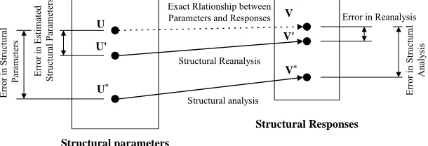
As indicated in Figure 1, the alteration quantity of structure response that corresponds to that of the struc-ture parameter generally tends to be smaller. Thus, to obtain the exact structural parameter of inverse problem that performs the damage detection by applying the sys-tem identification, the difference between the analytical response and the observed response should be obviously indicated. On the contrary, identifying the degree of damage through structure reanalysis belongs to the in-verse problem in a broader meaning. However, even though some error is included in the correlated analytical model obtained through the system identification, the error in the reanalyzed response is considerably reduced to describe the behavior of the real structure. This rela-tion is described in Equarela-tion (1),

*

U  V V  V (1)

where is the actual response of the structure, is the correlated analytical model, is the initial base-line model, and is the response modification value of actual observation. After all, in proportion to the ac-curacy of response modification value that applies the data actually observed in the structure, the real response of the structure can be predicted more efficiently.

U V

*

V V



3. Estimation Method for Model Updating

Consider an n-DOF, linear dynamic system of baseline model described by

 

 

 

 

,

My t Cy t Ky t  f t t0 (2)

where

 

N

y t R is the vector of generalized coordi-

nates,

 

N

y t R is the forcing vector, MRN N is

the symmetric, positive definite mass matrix, N N

CR 

is the symmetric, positive, semi-definite damping matrix,

and, N N

KR  is the symmetric, positive definite

stiff-ness matrix. The over-dot denotes differentiation with respect to time. The frequency response of Equation (2) is given by



2



 

 



M K y i Cy f



    

       (3)

where _{f t}

 

_{ f}

 

 _ei t _{and y t}

 

_y

 

 _ei t _{are used.}

If variable mass, stiffness and damping for model updat-ing are added, Equation (3) can be expressed as



 

  





 

 

2

M M K K y

i C C y f

 

  

      

 

   

 

 (4)

where, M , C and K are the n by n variable mass, damping and stiffness matrices for model updating, respectively. Due to physical limitations and time of cost constraints, however, the number of distinct parameters is almost always less than degrees of freedom of the analytical model. Thus, in practice, n < N. By the way,

M

 , C and K depend on the experimental

de-gree of freedom available in the observation experiment of dynamic system, overall system of structure can eventually be condensed in the degree of freedom which is identical to the experimental degree of freedom. Actu-ally, it is impossible to obtain the degree of freedom which is identical to that of the structure. Therefore, only the lower mode response that mainly represents the dy-namic system is observed. It is nothing but an approxi-mate solution, because it does not observe all response features of the overall structure system, but merely util-izes the value of the lower mode acquired in the experi-ment. However, if the value of the lower mode generally represents the structure in the case of civil engineering structures and if the value of the lower mode presents satisfactory measurements, this will not be largely dif-

Structural parameters

Structural Responses Exact Rlationship between

Parameters and Responses

Structural Reanalysis

Structural analysis

Er

ror in

Struc

tura

l

Par

ame

te

rs

E

rror

in E

stima

te

d

S

tr

uct

ur

al

P

ar

am

et

ers

Error in Reanalysis

Er

ro

r i

n S

tru

ct

ura

l

Ana

lysi

s

U' U

U*

V

V'

[image:2.595.147.452.588.692.2]

V*

ferent from the accurate values in which more modes are included, but will effectively lessen the degree of free-dom of the analytical structure. Thus, the error in calcu-lation can be reduced, with even higher efficiency, thanks to its reduced length. Since the term inside the parentheses represents the inverse of normal FRFs matrix, Equation (4) can be rewritten as

 

 

1 _N

 

_*N

   

y  _Ii B  _{ } H  H  f  (5)

where

 

N

 

*N

  



B  _H  H  _ CC (6) is referred to as the transformation matrix. It is noted that

 

B  is real matrix. where I is the identity matrix,



N

H 



is the frequency response function matrix of

baseline model generated from the normal modes, and



*N

H 



is the variable frequency response function

matrix for model updating generated from the normal modes. On the other hand, the complex frequency re-sponse equation of total dynamic system can also be represented as

 

TC

   

y  H  f  (7)

where TC

 

H  is the complex frequency response

function matrix of total dynamic system. And, it can be actually calculated actuality in the total structure system through an experiment. Note that N

 

H  is a square

matrix, since it is synthesized from the identified com-plex modes of total dynamic system by separating

 

N

H  into real and imaginary parts. Comparing Equ-

ations (5) and (7), the relationship between the FRFs for complex modes and normal modes is given by

 

 

 

 

 

 

*N TC _{( )} TC

R I

TC TC

R I

H H B H

i B H H

   

  

 

_   _

 

 _  _

N H

(8)

where TC

 

R

H  is the real part of a complex frequency

response function matrix of total dynamic system, and

 

TC I

H  is the imaginary part of a complex frequency

response function matrix. Since the left hand side of Equation (8) is a real matrix, so the imaginary part of the right hand side must be equal to a zero matrix for all frequencies and the transformation matrix then B

 



can be solved in terms of the matrices TC

 

R

H  and

 

TC I

H  by

 

TC

 

 

TC

 

I I

B   H  B  H  _HN ₍₉₎

Substituting Equation (9) into Equation (8) yields the relation between the normal FRFs matrix and the com-plex FRFs matrix as

 

 

 

 

*N TC TC N

R I

H  H  B  H  H (10)

From Equations (9) and (10), the transformation

ma-trix B

 

 and the variable normal FRFs matrix for

model updating *N

 

H  can be calculated,

respec-tively. Once matrices B

 

 and H*N

 

 become

available, the variable damping matrix for model updat-ing can be calculated from Equation (8). Finally, corre-lated frequency response function can be expressed by

 

TC R

H  and HTC_I

 

 of frequency response function

that can get in an experiment of total dynamic system. After all, by applying the FRFs that was obtained in the experiment of all structure system, the correlated ana-lytical model can be reorganized as a modification of the baseline analytical model. This means that the model, unlike the general dynamic analysis, can express the be-havior of a real structure more accurately. For a noise-free case, an exact solution for updated damping matrix can be obtained directly from Equation (6) by

 

1

 

1

* j j

j

C H N  B 





  C

  _{ }  (11)

where j is chosen frequency. In practice, the

fre-quency response functions are more or less contaminated with noise and the Least Square Method is employed to solve the updated damping matrix. It is noted that the updated damping matrix is identified independently from the mass and stiffness matrices. This is the main differ-ence from the other methods. Next, the identification of updated mass and stiffness matrices is presented. For an undamped system, the equation of motion can be written as





 



_2_{M K y }



_{ f}

 

_{ (12)}

The relation between the matrices, M , K and

 

*N

H  is given by





 



2 *N



M K H I

 

     (13)

where _H*N

 

 _{is calculated from Equation (10).}

Similar to the preceding section, the real overdetermined equation can be obtained and can also be solved by the least squares method.

4. Numerical Example

experimental data is to add proportional Gaussian ran-dom noise to FRFs where each datum is factored as

 

 

1



H  H  as (14)

where is a normally distributed variable, and s is a user-specified standard deviation. It is unlikely that genuine experimental noise will be either Gaussian of proportional. Arbitrary noises having noise levels of 5% - 10% are employed in the article.

a

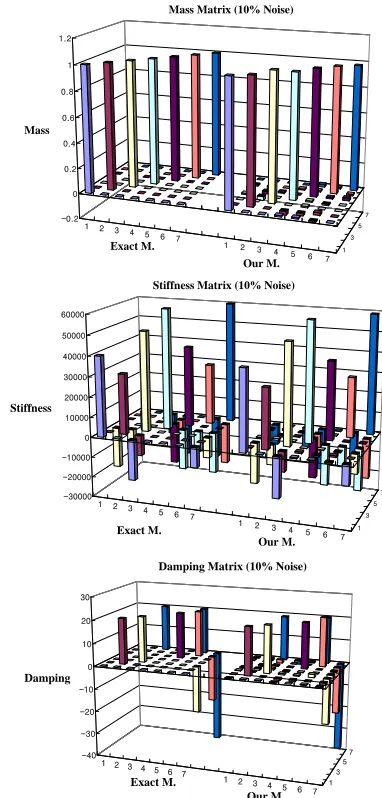
A sample structure employed in the numerical test II as Lembregts [11] suggested has totally 7 degrees of freedom. The shape of the structure is shown in the Fig-ure 2 and the dynamic properties are the same with Equation (15). In the selected sample structure, the third and the fourth modes, and the fifth and sixth modes form very close couples and the damping ratio of the sixth mode, 7% is largest. In conclusion the selected structure is of highly coupled system. In the numerical test, the initially assumed baseline finite element model was as-sumed to be 90% of true dynamic properties.

4

1 0 0 0 0 0 0 0 1 0 0 0 0 0 0 0 1 0 0 0 0 0 0 0 1 0 0 0 0 0 0 0 1 0 0 0 0 0 0 0 1 0 0 0 0 0 0 0 1

4 0 2 0 0 0 1

0 3 1 0 0 0 0

2 1 5 0 0 0 1

10

0 0 0 6 2 1 2

0 0 0 2 4 0 0

0 0 0 1 0 3 2

1 0 1 2 0 2 6

0 0 0 0 0 0 0

0 20 0 0 0 0 0

0 0 20 0 0 0 20

0 0 0 0 0 0 0

M K C                             _          _    _  _        _{   }     

0 0 0 0 20 0 0

0 0 0 0 0 20 20

0 0 20 0 0 20 40

                    _{ }    (15)

As the result of the analysis, it is known that in case of noise-free experimental data the dynamic properties of the estimated correlated finite element model correspond to true values of the structure, and even in case of the noise level of 5% satisfactory results are presented. Fig-ure 3 shows the dynamic parameters of the updated finite

m₁ m₁

k₁

k₁

k₁

k₁

k₁

k₁

k₁

k₁

k₁

k₁

k₁

k₁ k₁

k₁ k₂

k₂

k₂

k₂

k₂

k₂

k₂

k₂

k₂

k₂ c c c c c c c c

m2 m2

m₃ m₃

m5 m5

m4 m4

m₆ m₆

m₇ m₇

k₂

[image:4.595.312.537.77.262.2]

k₂

Figure 2. Updated system of 7 degrees of freedom.

1 2 3 4 5 6 7

1 2 3 4 5 6 7

1 3 5 7 -0.2 0 0.2 0.4 0.6 0.8 1 1.2 Mass

Mass Matrix (10% Noise)

Exact M.

Our M.

1 2 3 4 5 6 7

1 2 3 4 5 6 7

1 3 5 7 -30000 -20000 -10000 0 10000 20000 30000 40000 50000 60000 Stiffness

Stiffness Matrix (10% Noise)

Exact M.

Our M.

1 2 3 4 5 6 7

1 2 3 4 5 6 7 1 3 5 7 -40 -30 -20 -10 0 10 20 30 Damping

Damping Matrix (10% Noise)

Exact M.

[image:4.595.325.516.293.692.2]

Our M.

dated system properties necessary for correcting the ini-tially assumed baseline finite element model. It is known that the method can reduce significantly calculation error, and most importantly error accumulation arising in the calculation because the method estimates the updated damping matrix independently of the mass and the stiff-ness matrices while existing methods estimate the up-dated damping matrix while they consider both the mass and the stiffness matrices.

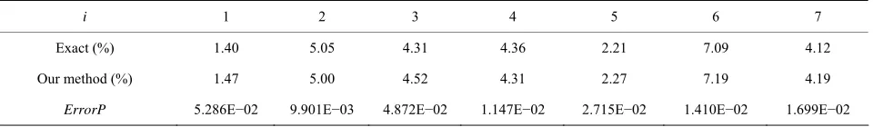
element model estimated at the noise level of 10%. The natural frequencies and the damping ratios according to the noise levels (5%, 10%) are indicated in Tables 1-4, where i is th number of modes. The errors are given by

Exact Updated ErrorP

Exact 

 (16)

for i = 1,2,3,4,5,6,7, where Error P denotes the relative errors induced by proposed method.

The proposed updating algorithms depend on the con-nectivities in the baseline finite element model to be cor- rect. Because the basis of model updating is the baseline finite element model, the baseline finite element model must capture certain physical attributes of the actual sys-tem. The proposed method, expanding the combination of FRF, can independently estimate the response modi-fication damping from FRF that is observed irrespective of mass matrix or stiffness matrix. Therefore, the accu-mulation of calculation error can be decreased consid-erably. The method suggested in this research does not seek, in one time, the dynamic parameters of structure by using data observed in the dynamic system, but suggests Generally the error which arises in estimating the

up-dated damping matrix is significantly larger than those of the updated mass and the stiffness matrices. It is because the damping effect is much smaller than the mass and stiffness matrices. To overcome this difficulty, the pre-sent effort succeeds in updating the damping matrix in-dependently from the updated mass and the stiffness ma-trices. This is the main difference between the present method and the existing methods. And the method sug-gested in the article is not to estimate at once the dy-namic properties of the structure by using the experi-mental data in the dynamic system but to present the correlated finite element model by estimating the up-

Table 1. Natural frequencies comparisons (5% noise level).

i 1 2 3 4 5 6 7

Exact (rad/sec) 13.40 22.89 28.15 28.88 40.85 41.38 45.99

Our method (rad/sec) 13.39 22.90 28.14 28.87 40.85 41.39 45.98

[image:5.595.56.540.370.526.2]

ErrorP 9.701E−04 5.679E−04 4.263E−04 3.809E−04 9.792E−05 3.142E−04 3.044E−04

Table 2. Natural frequencies comparisons (10% noise level).

i 1 2 3 4 5 6 7

Exact (rad/sec) 13.40 22.89 28.15 28.88 40.85 41.38 45.99

Our method (rad/sec) 13.36 22.93 28.12 28.85 40.86 41.41 45.96

[image:5.595.66.539.554.623.2]

ErrorP 2.687E−03 1.616E−03 9.236E−04 9.349E−04 3.427E−04 6.767E−04 5.653E−04

Table 3. Damping ratios comparisons (5% noise level).

i 1 2 3 4 5 6 7

Exact (%) 1.40 5.05 4.31 4.36 2.21 7.09 4.12

Our method (%) 1.37 5.03 4.4 4.32 2.19 7.13 4.08

[image:5.595.61.541.652.722.2]

ErrorP 2.143E−02 3.960E−03 2.088E−02 9.174E−03 9.050E−03 5.642E−03 9.709E−03

Table 4. Damping ratios comparisons (10% noise level).

i 1 2 3 4 5 6 7

Exact (%) 1.40 5.05 4.31 4.36 2.21 7.09 4.12

Our method (%) 1.47 5.00 4.52 4.31 2.27 7.19 4.19

correlated analytical model by identifying response mo- dification to supplement the initially assumed baseline analytical model. Thus, the error in calculation can be reduced considerably. Furthermore, while the existing methods estimate damping matrix by considering mass and stiffness simultaneously, this method identifies re-sponse modification damping irrespective of mass and stiffness matrix. Therefore, the accumulation of error in the calculation is notably reduced.

5. Conclusions

This article suggested the structural reanalysis method evaluating the correlated finite element model corrected by means of the FRFs of the structure. In conclusion, even with noise-mixed data, the suggested method could predict the updated structural system more accurately even with noise-mixed data. The proposed method, ex-panding the combination of FRF, can independently es-timate the response modification damping from FRF that is observed irrespective of mass matrix or stiffness ma-trix. Therefore, the accumulation of calculation error can be decreased considerably. Also, the results of the article can be properly utilized to evaluate the state of the dy-namic system necessary for the maintenance and man-agement of the structure or locate the positions to be modified.

6. References

[1] H. G. Natke, “Updating Computation Models in the Fre-quency Domain Based on Measured Data: A Survey,”

Probabilistic Engineering Mechanics, Vol. 3, 1988, pp.

8-35. doi:10.1016/0266-8920(88)90005-7

[2] R. M. Lin and D. J. Ewins, “Model Updating Using FRF Data,” Proceedings of ISMA, Vol. 15, 1990, pp. 141-163.

[3] M. Imregun and W. J. Visser, “A Review of Model Up-dating Techniques,” Shock and Vibration Digest, Vol. 23,

No. 1, 1991, pp. 9-20. doi:10.1177/058310249102300102 [4] J. E. Mottershead and M. I. Friswell, “Model Updating in

Structural Dynamics: A Survey,” Journal of Sound and Vibration, Vol. 167, 1995, pp. 347-375.

doi:10.1006/jsvi.1993.1340

[5] A. Bhasiar, S. S. Sahu and B. C. Nakra, “Approximations and Reanalysis over Parameter Interval for Dynamic De-sign,” Journal of Sound and Vibration, Vol. 248, No. 1,

2001, pp. 178-186. doi:10.1006/jsvi.2001.3686

[6] C. Mares, J. E. Mottershead and M. I. Friswell, “Stochas-tic Model Updating: Part 1—Theory and Simulated Ex-ample,” Mechanical Systems and Signal Processing, Vol.

20, No. 7, 2006, pp. 1674-1695. doi:10.1016/j.ymssp.2005.06.006

[7] C. Joao, N. D. Biswa, G. Abhijit and L. Maitreya, “A Direct Method for Model Updating with Incomplete Measured Data and without Spurious Modes,” Mechani-cal Systems and Signal Processing, Vol. 21, No. 7, 2007,

pp. 2715-2731. doi:10.1016/j.ymssp.2007.03.001

[8] E. Capiez-Lernout and C. Soize, “Robust Updating of Uncertain Damping Models in Structural Dynamics for Low- and Medium-Frequency Ranges,” Mechanical Sys-tems and Signal Processing, Vol. 22, No. 8, 2008, pp.

1774-1792. doi:10.1016/j.ymssp.2008.02.005

[9] V. Arora, S. P. Singh and T. K. Kundra, “Further Ex-perience with Model Updating Incorporating Damping Matrices,” Mechanical Systems and Signal Processing,

Vol. 24, No. 5, 2010, pp. 1383-1390. doi:10.1016/j.ymssp.2009.12.010

[10] S. R. Ibrahim and A. Sestieri, “Analysis of Errors and Approximations in the Use of Modal Coordinates,”

Journal of Sound and Vibration, Vol. 177, No. 2, 1994,

pp. 145-157. doi:10.1006/jsvi.1994.1424

[11] F. Lembregts and M. Brughmans, “Estimation of Real Modes from FRFs via Direct Parameter Identification,”