University of Warwick institutional repository
This paper is made available online in accordance with publisher policies. Please scroll down to view the document itself. Please refer to the repository record for this item and our policy information available from the repository home page for further information.
To see the final version of this paper please visit the publisher’s website. Access to the published version may require a subscription.
Author(s): William J. Matthews and Neil Stewart
Article Title: The effect of interstimulus interval on sequential effects in absolute identification
Year of publication: 2009 Link to published version :
The effect of inter-stimulus interval 1
The effect of inter-stimulus interval on sequential effects in absolute identification
William J. Matthews
and
Neil Stewart
University of Warwick
RUNNING HEAD: Sequential effects
Address correspondence to:
William Matthews
Department of Psychology,
University of Warwick,
Coventry
CV4 7AL
UK
Tel: +44/0 24 765 23096
Fax: +44/0 24 765 24225
Email: [email protected]
Matthews, W. J., & Stewart, N. (2009). The effect of inter-stimulus interval on sequential
Abstract
In absolute identification experiments, the participant is asked to identify stimuli drawn from a small set of items which differ on a single physical dimension (e.g., ten tones which vary in frequency). Responses in these tasks show a striking pattern of sequential dependencies: The current response assimilates towards the immediately preceding stimulus but contrasts with the stimuli further back in the sequence. This pattern has been variously interpreted as resulting from confusion of items in memory, shifts in response criteria or the action of selective attention, and these interpretations have been incorporated into competing formal models of absolute
identification performance. In two experiments, we demonstrate that lengthening the time between trials increases contrast to both the previous stimulus and the stimulus two trials back. This surprising pattern of results is difficult to reconcile with the idea that sequential
dependencies result from memory confusion or from criterion shifts, but is consistent with an account which emphasizes selective attention.
The effect of inter-stimulus interval on sequential effects in absolute identification
On each trial of an absolute identification experiment, the participant is required to identify a stimulus drawn from a small set of items which differ on a single physical dimension (e.g., 10 tones which differ only in intensity). It has long been known that absolute identification data exhibit several interesting phenomena, including a severe limit in information transmission between stimuli and responses (e.g., Miller, 1956) and greater accuracy for stimuli at the ends of the stimulus range than in the middle (e.g., Murdock, 1960), and in the past few years there has been a resurgence of interest in absolute identification research (Brown, Marley, Donkin, & Heathcote, 2008; Brown, Marley, & Lacouture, 2007; Kent & Lamberts, 2005; Petrov & Anderson, 2005; Rouder, Morey, Cowan, & Pfaltz, 2004; Stewart, 2007; Stewart, Brown, & Chater, 2005).
A key result from absolute identification experiments is the finding that the response on
the current trial R to the presented stimulusn S depends upon the sequence of preceding stimuli.n
Typically, R assimilates towards the immediately preceding stimulusn Sn1 but contrasts with
(i.e., shifts away from) the stimuli presented two or more trials back (Sn2,Sn3…). The
magnitudes of these effects, and the point in the sequence at which there is a switch from assimilation to contrast, depend upon the difficulty of the task and whether or not feedback is provided (e.g., Ward & Lockhead, 1971), but the basic pattern has been found in a large number of studies (Holland & Lockhead, 1968; Lacouture, 1997; Luce, Green, & Weber, 1976, analysed in Jesteadt, Luce, & Green, 1977; Staddon, King, & Lockhead, 1980; Stewart et al., 2005;
Over the past 40 years, this pattern of sequential effects has been given a number of different psychological interpretations, and these interpretations have been incorporated into competing formal models of absolute identification. Broadly speaking, the explanations for the sequential dependencies fall into three groups, which we now discuss in turn. Throughout, we focus on thecore psychological ideas rather than detailed discussion of formal models, not least because recent models (e.g., Brown et al., 2008; Stewart et al., 2005) incorporate many free
parameters and may possibly, with appropriate parameter choices, be rendered indistinguishable.
The first interpretation of sequential effects is that they represent the confusion of items in memory. This idea was first proposed by Holland and Lockhead (1968) and has appeared in various forms since then (Lockhead & King, 1983; Lockhead, 1984; 1992). According to this interpretation, the representation of each stimulus is confused with the memories for earlier stimuli in the trial sequence. More recently, Stewart et al. (2005) have incorporated the idea of memory-confusion into a highly successful model which captures the full set of absolute identification choice data, including sequential effects. According to Stewart et al.’s relative judgment model (RJM), the participant estimates the difference between the current stimulus and the previous one (Laming, 1984). This difference is added to the feedback from the previous trial to produce a judgment of the current stimulus, with noise in the mapping of the perceived
on the response scale is approximately correct, the confusion of stimulus differences predicts
assimilation to Sn1 and contrast to stimuli further back.
Memory-confusion interpretations of sequential effects like those of Stewart et al. (2005) suggest that the current response is predicted by the preceding stimulus sequence; preceding
responses are ignored. The dependence ofR on the current and preceding stimuli mayn
conveniently be assessed by fitting a regression equation to the data:
n k n k n
n n
n r S S S S e
R 0 D0 D1 1D2 2...D (1)
Because only preceding stimuli are included as predictors in Equation 1, we refer to it as a stimulus-only regression. When Equation 1 is applied to absolute identification data, the
coefficient for Sn1is positive, indicating assimilation, and the coefficients for stimuli further
back in the sequence are negative, indicating contrast (e.g., Lockhead, 1984).
The second interpretation of sequential effects is that they represent trial-by-trial shifts in response criteria. A comprehensive statement of this idea is provided by criterion setting theory (Triesman & Williams, 1984; Treisman, 1985). Criterion setting theory adopts a Thurstonian framework in which the presentation of each stimulus results in a noisy value on an internal sensory scale. Criteria, or response boundaries, divide the sensory scale into response categories and the response is determined by which criteria the (noisy) stimulus representation falls
between. Each criterion has a long-term reference location, but the effective criteria on each trial are also influenced by two short-term processes: tracking and stabilization. The tracking
involves shifting the criteria away from the most recently made response, increasing the probability that the response will be repeated. Thus, the tracking mechanism produces
assimilation to recent responses. The stabilizing mechanism, on the other hand, serves to place criteria near to the prevailing flux of sensory input. For example, if a series of sensory inputs all lie well above a criterion then that criterion may be too low in relation to the current distribution of inputs. Stabilization therefore shifts each criterion towards the current sensory input,
producing contrast to recent stimuli.
Criterion setting theory thus asserts separate effects of preceding stimuli and preceding responses, with contrast to the former and assimilation to the latter. These effects suggest that absolute identification data may usefully be described with a regression equation in which both stimuli and responses are included as predictors:
n k n k k n k n n n
n r S S R S R e
R 0 D0 D1 1E1 1...D E (2)
Because both preceding stimuli and preceding responses are included as predictors, we refer to Equation 2 as a stimulus-response regression. (Note that the term stimulus-response regression should not be taken to imply that the effects of preceding stimuli and responses are linked, only that both factors are being considered as predictors of the current response.) Mori and Ward (1995) applied a version of Equation 2 to absolute identification data and found that, in keeping
with criterion setting theory, the coefficient for Rn1 was positive but that the coefficient for Sn1
was often negative, most notably in the absence of feedback - although the high correlation of stimuli and responses means that these coefficients may not be reliable. Mori (1998) similarly
the stimuli were masked. Both of these studies only considered the effects of the immediately preceding trial (Jesteadt et al., 1977).
The third interpretation of sequential effects is that they result from the operation of selective attention (e.g., Luce et al., 1976). Selective attention forms the basis of a recent, highly successful account of absolute identification - the selective attention, mapping, ballistic
accumulator (SAMBA) model of Brown et al. (2008). SAMBA is able to predict the full range of choice and RT data from absolute identification experiments. At the heart of the model is a selective attention mechanism based on the rehearsal process of Marley and Cook (1984; 1986). It is assumed that the stimulus dimension is monotonically mapped onto a linearly ordered set of leaky nodes. Throughout the experiment the participant rehearses a region of the stimulus dimension by directing rehearsal activity to a subset of these nodes. The upper and lower nodes in this range are referred to as anchors; their positions depend upon the range of stimuli in the experiment. To produce a magnitude estimate for the current stimulus the participant judges the position of the stimulus within the rehearsed range by calculatingL, the total rehearsal
takes to do so determines the RT.
It is clear from the foregoing survey that, while sequential effects provide a strong empirical constraint on formal models of absolute identification, the psychological interpretation of these effects remains disputed. In the current paper, we seek to clarify the interpretation of sequential dependencies by asking how the effects of previous stimuli and responses depend upon the time interval between trials. Manipulations of inter-stimulus interval have proved useful in distinguishing between interpretations of sequential effects in other tasks (e.g., Collier, 1954; DeCarlo, 1992) and several authors have recently argued for the importance of manipulating inter-stimulus interval in absolute identification (Brown et al., 2008; Lockhead, 2004; Stewart et al., 2005). The two experiments reported here represent the first attempt to do so.
Experiment 1
Method
Participants
Thirty nine members of the University of Warwick subject panel took part. Each was paid £12.
Stimuli
including a 50-ms amplitude ramp at beginning and end. Tones were played over Sennheiser eH2270 or HD265 headphones.
Design and Procedure
(blank) = 5000ms whilst in the Long condition it was 3000 + 500 + 5500 + 500 + 500 = 10000ms. The experiment was controlled by DMDX (Forster & Forster, 2003).
All participants had a break between sessions and some chose to come back on a different day to complete the second session. The first block of trials from each session was treated as practice and excluded from the analysis.
Results and Discussion
One participant was discarded because of technical difficulties; a second was discarded because of failing to respond within the 3s response window on a large proportion (14.1%) of trials (the mean proportion for the remaining subjects was 1.0%). For two of the 37 useable participants, one block of trials was discarded because the test session was briefly interrupted; 18 participants completed the sessions in the order Short-Long and 19 in the order Long-Short.
Basic Performance
The average proportion of trials on which the participant failed to respond in the 3s window in the Short condition was 0.7% (SD = 1.0); the mean for the Long condition was 1.4% (SD = 1.7). We used a mixed ANOVA to examine the effects of ISI and session order (Short-Long or Long-Short) on the proportion of missed responses. There was a main effect of condition, F(1,35) =
6.70, K2p = .16, p = .014, with significantly more missed responses in the Long condition than
the Short condition. (Here and throughout what follows, the criterion for significance was set at 05
.
responses in both conditions indicates that our choice of a 3s response window was appropriate. There was no effect of session order, F(1,35) < 1, and no interaction, F(1,35) < 1. The mean proportion of correct responses (excluding missed responses) in the Short condition was 54.0% (SD = 10.3), the mean for the Long condition was 52.7% (SD = 10.5). Analysis of variance
indicated no effect of condition, F(1,35) = 1.37, K2p = .04, p = .249, no effect of session order,
F(1,35) < 1, and no interaction, F(1,35) < 1.
In short, analysis of accuracy and proportion of missed trials shows that these statistics vary only slightly with changes in ISI and do not compromise the analysis of sequential effects which are the main focus of the current paper.
Sequential Effects
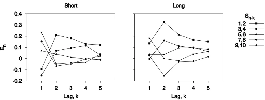
The effects of the preceding stimulus sequence on the current response are illustrated in Figure 1. This figure provides a so-called “impulse plot” (e.g., Lockhead, 1984). In an impulse plot, the
mean error on the nth trial (averaged across all S ) is shown as a function of the lag, k, for alln
possible Snk. The left panel shows the results from the Short ISI condition; the right panel
shows the results from the Long ISI condition. (As is usual, the data have been collapsed over pairs of stimuli.)
Consider first the data from the Short condition. There is assimilation to the stimuli presented at lag k = 1, because the mean error on trial n is positive when the stimuli presented on trial n-1 are large, and negative when the stimuli presented on trial n-1 are small. However, the
effect of stimuli shown at lag k = 2 is the opposite; when Sn2 was large, the mean error on trial
stimuli at longer lags. The left panel of Figure 1 therefore illustrates the classic pattern of
assimilation to Sn1 and contrast to Sn2 seen in many previous studies of absolute identification
(e.g., Lockhead, 1984; Stewart et al., 2005; Ward & Lockhead, 1970; 1971) When we turn to the results from the Long ISI condition, however, two differences are apparent. Firstly, the
assimilation to Sn1 has disappeared and, if anything, been replaced by weak contrast. Secondly,
the magnitude of the contrast to Sn2, and possibly to stimuli further back in the sequence, has
increased. Figure 1 therefore suggests that increasing the ISI has led to a general increase in contrast.
Impulse plots provide a convenient way to visualise the data, but they do not permit a quantitative analysis. Moreover, they do not separate the effects of preceding stimuli and preceding responses. We therefore fit Equations 1 and 2 to the data, to obtain a clearer understanding of the effects of inter-stimulus interval on sequential effects.
Stimulus-only regression
We began by fitting the stimulus-only regression equation (Equation 1) using stimuli up to five trials back in the sequence as predictors. (Responses which fell outside the 3s response window were excluded from the analysis.) We conducted the regression analysis separately for both the Short and Long ISI conditions for each participant and then compared the regression coefficients from the two conditions. (An alternative approach would be to include the data from both
conditions in a single regression which included ISI and the interactions between ISI and the
various Snkterms as predictors. The pattern of results from such an analysis are identical to
participants are presented in the left of Table 1. Inspection of the regression coefficients reveals
the same pattern as Figure 1. In the Short ISI condition, the coefficient for Sn1 is moderately
large and positive, indicating assimilation, whilst the coefficient for Sn2 is negative, indicating
contrast. In the Long ISI condition, the coefficient for Sn1 has dropped to slightly below zero,
whilst the coefficient for Sn2 has become more negative. Finally, we note that the fit of the
regression equation is good ( 2
R approximately .85), and little affected by the ISI condition. This is true of all of the regression equations fit in both experiments.
As one would expect when a large number of participants complete only a few hundred trials each, there was individual variation in the regression coefficients. We therefore used analysis of variance to statistically test the effects of ISI on the regression coefficients (Lorch & Myers, 1990)1. We conducted a mixed ANOVA with ISI (Short vs. Long) as a within-subject factor and session order (Short-first vs. Long-first) as a between subjects factor. (Throughout what follows, the effects of session order were not significant unless otherwise stated.) The right side of Table 1 shows the ANOVA results for the main effect of ISI on each coefficient. The
results show that inter-stimulus interval exerted a significant effect on the coefficients for Sn1
and Sn2; increasing the ISI significantly reduced assimilation to Sn1 and significantly
increased contrast to Sn2. The coefficients for stimuli further back in the trial sequence were not
significantly affected by the ISI manipulation.
To investigate the separate effects of preceding stimuli and responses, we applied Equation 2 to the data from Experiment 1. For this analysis, we considered the effects of stimuli and responses from the previous two trials. The mean and standard deviations of the regression coefficients are shown in the bottom of Table 1. Also shown at the right of the table are the ANOVA results for the main effect of ISI condition.
The coefficient for Sn1 is significantly influenced by the inter-stimulus interval. In the
Short condition, it is close to zero; in the Long condition, it is markedly negative, indicating a
shift to contrast as the ISI is increased. A similar pattern is found for Sn2, with contrast in the
Short condition becoming significantly more pronounced in the Long condition (although the p value for this effect is not particularly small; as a general point in the current work, we suggest that any significant results for which the p value is not considerably less than .05 be treated with some caution). The effects of previous responses are not influenced by ISI. There is moderate
assimilation to Rn1 and very little effect of Rn2, neither of which is influenced by the ISI
manipulation. There was also a significant main effect of session order for the Rn2coefficient,
F(1,35) = 5.20, p = .029, K2p= .13, although session order did not interact with experimental
condition, F(1,35) = 1.41, p =.243, 2
p
K = .04. This result is hard to interpret, and we do not
consider it further.
In short, increasing the ISI makes the coefficients for both Sn1 and Sn2 more negative.
That is, in the Long condition, there is stronger contrast to preceding stimuli than in the Short condition2.
The results of Experiment 1 show that, irrespective of which regression model is used to assess the sequential effects, increasing the time between trials increases contrast to preceding stimuli. This is a novel and counter-intuitive result with strong theoretical implications, which we discuss below. Before that, we report a second experiment which sought both to establish the generality of this finding and to dissect the influence of intervals between specific pairs of trials.
Experiment 2
In Experiment 1, the Short and Long ISI conditions were grouped into blocks of trials. In Experiment 2, short and long inter-stimulus intervals were randomly intermixed throughout the experiment. The motivation for this was twofold. Firstly, we sought to replicate the striking pattern of results obtained in Experiment 1 under different conditions. Secondly, we sought to clarify which inter-stimulus intervals contribute to the observed effects. For example, in
Experiment 1 it was found that increasing the ISI caused increased contrast to Sn2. Was this
because of the increased interval between Sn2 and Sn1, the increase between Sn1 and S , orn
both? Randomly intermixing short and long inter-stimulus intervals throughout the trial sequence allows us to answer this type of question.
Method
Thirty eight members of the University of Warwick subject panel took part. Each was paid £6.
Stimuli
The stimuli were the same as Experiment 1.
Design & Procedure
Each participant completed a single experimental session consisting of five blocks of 80 trials. In each block, each of the ten tones was presented eight times, four times followed by a short ISI and four times followed by a long ISI. The order was randomized for each participant.
At the start of the experiment, the ten tones were played in sequence from 1-10 with a 1s gap between each. While the tones played, the corresponding numbers appeared on the computer screen. Participants then began the experimental trials. On each trial, participants heard one of the 10 tones; after the tone had finished, the participant had 2.5 seconds to indicate which of the tones had played by pressing one of the number keys along the top of a standard computer keyboard. At the end of the response window, the actual number of the presented tone was displayed for 500ms. On trials where participants failed to make a response, the words ‘Too slow’ were presented with the numerical feedback. Following the feedback there was a blank interval of 500ms (short ISI) or 5000ms (long ISI) after which the word ‘Ready’ was shown for 500ms followed by a further 500ms blank interval before the next tone played.
short ISI condition and 2500 + 500 + 5000 + 500 + 500 = 9000 ms in the long ISI condition. The first block of trials from each session was treated as practice and excluded from the analyses.
Results and Discussion
Two participants failed to respond within the 2.5s window on a large proportion of trials (19.9% and 20.8%) and were excluded from the analysis; the mean proportion of missed responses for the remaining participants was 1.5%.
We refer to the interval between Sn2 and Sn1as ISIn2,n1, and to the interval between
1
n
S and S asn ISIn1,n. The data were organized according to ISIn2,n1and ISIn1,n. For each
trial, the lengths of ISIn2,n1and ISIn1,nwere established and the data organized into the four
possible combinations of the two ISIs: S,S (i.e., both ISIs were short:ISIn2,n1 = 4.5s and ISIn1,n
= 4.5s), S,L (a short ISI followed by a long ISI,ISIn2,n1 = 4.5s, ISIn1,n = 9s), L,S (ISIn2,n1 =
9s, ISIn1,n = 4.5s) and L,L (ISIn2,n1 = 9s, ISIn1,n = 9s). Note that we label the conditions to
reflect, from left to right, the order in which the intervals were experienced. Thus condition S, L
corresponds to the stimulus sequence: Sn2 - short interval - Sn1 - long interval - S . In order ton
have a useable number of trials in each condition, the length of the ISI separating Sn3 and
2
n
S was ignored, as were other ISIs further back in the sequence.
The proportion of trials on which each participant failed to respond was calculated for each ISI condition. In condition S,S the mean proportion was 1.0% (SD = 1.5); in condition S,L the mean was 1.6% (SD = 2.3); in condition L,S the mean was 1.2% (SD = 1.5) and in condition L,L the mean was 2.1% (SD = 2.7). A 2x2 within-subject ANOVA revealed a marginally significant
effect of ISIn2,n1, F(1,35) = 4.13, p = .050, 2
p
K = .11, and a significant effect of ISIn1,n, F(1,35)
= 8.28, p = .007, 2
p
K = .19, but no interaction, F(1,35) < 1. As in Experiment 1, the overall
proportion of missed responses was very low, indicating that the choice of response window (2.5s) was appropriate. The mean proportion of correct responses (excluding missed responses) was also calculated for each condition. In condition S,S, the mean was 54.1% (SD = 14.9); in condition S,L the mean was 52.1% (SD = 12.6); in condition L,S the mean was 53.2% (SD = 14.2); in condition L,L the mean was 51.1% (SD = 13.1). A 2x2 within-subjects ANOVA
revealed no significant effect ofISIn2,n1, F(1,35)=1.16, p = .289, 2
p
K = .03, or ISIn1,n, F(1,35) =
3.66, p = .064, K2p= .09, and no interaction, F(1,35) < 1.
Sequential Effects
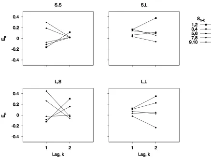
As in Experiment 1, we begin by considering impulse plots for each of the four conditions. These are shown in Figure 2. The top left panel shows the results when both intervals were short. There is assimilation to Sn1 and weak contrast to Sn2. The bottom left panel shows the results when
the interval between Sn2 and Sn1 was long and the interval between Sn1 and S was short.n
The assimilation to Sn1 has not changed, but the contrast to Sn2 has become more pronounced.
interval between Sn1 and S was long. Now the assimilation ton Sn1 has been replaced by weak
contrast; there is also contrast to Sn2, and the magnitude of this effect is similar to that seen in
condition L,S. Finally, the bottom right panel shows the results when both intervals are long. As
in the preceding condition, there is weak contrast to Sn1, and contrast to Sn2 which is even
stronger than before.
To quantify these findings, we again fit Equations 1 and 2 to the data.
Stimulus-only regression
For each of the four ISIn2,n1, ISIn1,n combinations, we fit a stimulus-only regression model
(Equation 1) to the data from each participant. The mean and standard deviations of the
regression coefficients for the 36 participants are presented in the upper portion of Table 2. (As in Experiment 1, an alternative approach is to conduct a single regression for the data from all
four conditions with the inclusion of interaction terms to assess the effects of ISIn2,n1
andISIn1,n. The results are identical to those reported here.)
The coefficients were entered in a 2x2 within-subject ANOVA. The upper portion of
Table 3 shows the F values, p values, and effect sizes for the main effects of ISIn2,n1 and
n n
ISI 1, and for the interaction term. For the S coefficient, there is a main effect ofn ISIn1,nand
an ISIn2,n1*ISIn1,n interaction. When ISIn2,n1 is short, the coefficient is unaffected by
n n
ISI 1, . When ISIn2,n1is long, the S coefficient is larger whenn ISIn1,n is long than when
n n
pattern suggested by inspection of the impulse plots in Figure 3: There is a main effect of ISIn1,n
on the coefficient for Sn1, but no effect of ISIn2,n1 and no interaction. Both ISIn2,n1 and
n n
ISI 1, significantly affect the coefficient for Sn2, but again there is no interaction. The lack of
interaction between the effects of ISIn2,n1 and ISIn1,nsuggests that it is the total amount of time
since Sn2was presented that determines the extent of contrast to this stimulus – i.e., the effects
of ISIn2,n1and ISIn1,nare additive.
Stimulus-response regression
We next applied a stimulus-response regression (Equation 2). The means and standard deviations of the regression coefficients are presented in the lower part of Table 2. A series of 2x2
within-subject ANOVAs were used to examine the effects of ISIn2,n1and ISIn1,non each coefficient
and the results are shown in the lower half of Table 3. The pattern for Sn is the same as for the
stimulus-only regression. For the Sn1coefficient, there is a main effect of ISIn1,n; when the
interval between Sn1 and S is short (i.e., in conditions S,S and L,S), there is weak assimilationn
to Sn1, but when the interval is long the coefficient becomes negative, indicating contrast. There
is no main effect of ISIn2,n1 and no interaction. The coefficient for Rn1 is moderately large and
positive in all conditions; there is no effect of ISIn1,n, no effect of ISIn2,n1, and no interaction.
That is, assimilation to Rn1 seems to be unaffected by inter-stimulus interval. Similarly, there is
contrast to Sn2 in all conditions. Inspection of the values for this coefficient suggests an
condition S,S and largest in condition L,L, with S,L and L,S having intermediate levels of
contrast. However, the ANOVA indicates no effect of ISIn1,n, no effect of ISIn2,n1, and no
interaction. It seems likely that the effect of inter-stimulus interval on the coefficient for Sn2 is
no longer significant because of the increased noise in the regression parameters due to the multicollinearity among the stimulus and response predictors. (Recall also that the pattern of
increasing contrast to Sn2 seen here was found to be significant in Experiment 1, where there
were more trials in each condition.) Finally, there is some evidence of weak assimilation to Rn2,
but as for Rn1 there is no effect of ISIn1,n, no effect of ISIn2,n1, and no interaction.
Summary
The results of Experiment 2 replicate those of Experiment 1. Both the stimulus-only and stimulus-response regression analyses indicate that increasing the time between trials increases
contrast to preceding stimuli. In addition, the effect of Sn1 depends only on ISIn1,n, whilst the
effect of Sn2 depends on both ISIn1,n and ISIn2,n1.
General Discussion
function of the preceding stimuli (ignoring previous responses, Equation 1), there was
assimilation to Sn1and contrast to stimuli further back in the sequence (e.g., Ward & Lockhead,
1970). However, when the ISI was increased to 10s the assimilation to Sn1disappeared whilst
the contrast to Sn2 became more marked. That is, for both Sn1 and Sn2there was a shift
towards contrast. When the effects of preceding responses were also considered (Equation 2), the Short ISI condition indicated very little effect of Sn1and contrast to Sn2, and the Long ISI
condition showed a significant increase in contrast to both Sn1and Sn2. There was also
evidence of assimilation to Rn1which was unaffected by the time between trials. Experiment 2
replicated these findings, and additionally found that the effects of Sn1 and Sn2 depend the
total time since their occurrence.
As we described above, sequential effects have variously been interpreted as resulting from memory confusion, from shifts in Thurstonian response criteria, or from selective attention. The surprising pattern of results found here imposes an important constraint on the psychological interpretation of sequential effects and on the formal models of absolute identification which incorporate these ideas. In what follows, we discuss these interpretations in turn and ask whether each can accommodate the pattern of results found in the two experiments.
Memory confusion
As described in the Introduction, sequential effects have long been taken to indicate the confusion of items in memory (e.g. Holland & Lockhead, 1968). The most successful
judged relative to the previous one but with the judgment of the current stimulus difference contaminated by memory for previous differences. Existing memory-based interpretations of sequential dependencies emphasize the effects of preceding stimuli and ignore previous responses; the impulse plots and stimulus-only regression analyses therefore provide the appropriate description of the data for appraising the memory-confusion account.
The results of these analyses are difficult to reconcile with a memory-based interpretation of sequential effects. If sequential effects reflect the influence of memories for previously
encountered stimuli, we would expect that influence to decrease as the time since the presentation of those stimuli is lengthened, because the memory trace fades over time (e.g., Wicklegren, 1974). This is true irrespective of whether the sequential effects result from memory for actual stimuli or from memory of stimulus differences. Even if one assumes that forgetting occurs over items rather than in physical time (e.g., McGeoch, 1932), the best that can be expected is that increasing the ISI will make no difference to the effects of previous stimuli. In
Experiments 1 and 2, increasing the time between trials decreased assimilation to Sn1, consistent
with the idea that the memory for that stimulus diminished. However, contrast to Sn2 became
more pronounced, not less.
It might be premature to abandon Stewart et al.’s (2005) highly successful account of absolute identification on the basis of the current results. However, we can see no
straightforward memory-based interpretation of the finding that increasing the time between trials diminishes the effect of the more recently presented stimulus but increases the effect of the more distantly presented item. Furthermore, the situation is not improved by asserting separate effects of preceding stimuli and responses. The stimulus-response regressions show that
why lengthening the time since the establishment of a memory trace should increase the effect of that trace on the current response.
Shifts in response criteria
The current data are also hard to reconcile with the idea that sequential effects result from shifts in Thurstonian response criteria. According to criterion setting theory (Treisman & Williams, 1984), each trial establishes a tracking trace which shifts the response criteria away from the current response, and a stabilization trace which produces a smaller shift towards the current stimulus. These traces decay over time so that the criteria move back to their long-term reference locations. Criterion setting theory therefore predicts separate effects of recent stimuli and
responses, with contrast to the former and assimilation to the latter. Increasing the time between trials should reduce both the assimilation to preceding responses and the contrast to preceding stimuli, and the stimulus-response regression analyses provide an appropriate description of the data against which to test these predictions.
The results of these analyses contradict criterion setting theory. In keeping with the
model, we found assimilation to Rn1; the magnitude of this effect was not affected by the ISI,
but this may simply reflect a slow decay in the tracking trace. However, we also found that
increasing the time between trials rendered the regression coefficients for Sn1 and Sn2
Criterion setting theory is, of course, only one instantiation of the idea that sequential effects result from shifts in response criteria. Alternative criterion-setting models could be developed to account for the current data if one were willing to assume arbitrary shifts in response criteria. Specifically, one would need to postulate shifts which initially increased over time (to explain the increase in contrast with increasing inter-stimulus interval) but which eventually changed direction and began to decay (because it makes no sense for the criteria to drift apart indefinitely). It would be hard to motivate such assumptions: Whereas Treisman and Williams (1984) convincingly argue that the shifts in criteria predicted by criterion setting theory tune the response system to the prevalent flux of sensory information, it is difficult to see how the pattern of criterion shifts needed to explain the current data could be justified.
Selective attention
Our results are hard to interpret in terms of memory processes or shifts in response criteria. They are, however, consistent with an account based on selective attention, the SAMBA model of Brown et al. (2008). Like criterion setting theory, this account posits separate influences of preceding stimuli and responses such that a stimulus-response regression provides the most appropriate description of sequential effects, and, as we have shown, the results of such analysis show that increasing the time between trials produces an increase in contrast to both Sn1 and
2
n
S . This is the pattern of results predicted by Brown et al.’s model.
series of nodes and the participant directs rehearsal activity to the nodes covering the range of stimuli presented during the experiment (Marley & Cook, 1984). Increments in the activity of each node are offset by a passive decay process, and the magnitude of a given stimulus is judged by determining the proportion of total rehearsal activity which lies below (or above) the
corresponding node. On some proportion of trials, the rehearsal activity is preferentially directed towards the most recently presented stimulus; this preferential rehearsal may also be considered a form of selective attention. If a subsequent stimulus lies above the preferentially-rehearsed node, the stimulus magnitude will be overestimated; if it lies below, the magnitude will be underestimated. Thus, preferential rehearsal of recent stimuli produces contrast to those stimuli.
This model predicts that contrast will increase with increasing ISI. Immediately after the
presentation of Sn1, the participant begins to direct rehearsal activity to the corresponding node.
Meanwhile, the activity in all the other nodes passively decays. The longer this goes on, the
greater the proportion of total rehearsal activity accruing to the Sn1node and, correspondingly,
the greater the contrast effect. There will also be increased contrast to Sn2, provided the model
parameters are chosen such that the increased rehearsal of the Sn2 node during the interval
between Sn2 and Sn1is not offset by increased decay during the interval between Sn1 and Sn
(or if, as Brown et al., 2008, suggest, the redirection of rehearsal activity continues for more than one trial.) The selective attention mechanism embodied in Brown et al.’s SAMBA model
this effect is predicted to decrease over time. The current experiments found the predicted response assimilation, and although we did not observe a decline in this effect when the ISI was increased this may simply reflect a slow decay in ballistic accumulator activity. Crucially, the selective attention mechanism is not tied to the other elements of SAMBA. The selective
attention component of SAMBA represents a general idea which may be incorporated into other psychophysical models, including ones which provide different explanations for response assimilation.
The selective attention component of SAMBA provides the only account of sequential effects which correctly predicts that increasing the ISI will increase contrast to preceding stimuli. However, there is one aspect of the current data which is potentially problematic for this account,
namely that the stimulus-response regression analyses provide little evidence for contrast to Sn1
in the short ISI conditions. In Experiment 1, the mean coefficient for Sn1 in the Short condition
was 0.009 (Table 1). In Experiment 2, the stimulus-response regression produced mean
coefficients for Sn1 of 0.030 in the S,S condition and 0.029 in the L,S condition (see the lower
half of Table 2). One sample t-tests established that none of these coefficients are significantly
different from zero. Mori and Ward (1995) similarly found that the coefficients for Sn1were
sometimes positive, although they are typically strongly negative in the absence of feedback (see also Mori, 1998). We do not regard this as a serious problem because the selective attention
mechanism is only expected to produce weak contrast to Sn1 when the ISI is short, and the
coefficients obtained from the stimulus-response regression used to identify stimulus-specific effects are noisy because of the multicollinearity among stimuli and response predictor variables. However, should future experiments find significant assimilation to Sn1 (when Rn1 is included
The current results have applicability beyond absolute identification. DeCarlo (1992) varied the ISI in a magnitude estimation experiment and found that, when a stimulus-response
regression was used, there was contrast to Sn1 which became more pronounced as the ISI
increased. DeCarlo suggested that this pattern indicated a mis-specification of the regression model. However, the selective attention component of SAMBA produces a magnitude estimate and Marley and Cook (1986) developed a model for magnitude estimation based upon this mechanism but without the redirection of rehearsal activity which produces contrast. If the re-direction of rehearsal activity to recently presented stimuli assumed by SAMBA also occurs in magnitude estimation experiments, then this might provide an explanation for DeCarlo’s result. That is, in magnitude estimation, as in absolute identification, preferential rehearsal of recent items may produce contrast to preceding stimuli, the magnitude of which increases with
increasing time between trials. Similarly, the current results argue against the idea that sequential effects result from confusion of items in memory or shifts in response criteria. Both of these ideas have been invoked as explanations for sequential effects in other psychophysical tasks (e.g., Lockhead, 1992; 2004; Treisman, 1984; Treisman & Williams, 1984); their failure to capture the pattern in absolute identification casts doubt on their applicability in these situations, too.
Acknowledgments
Footnotes
1
When separate regression analyses are conducted for a number of different participants, it is common to use inferential statistics, such as t-tests and ANOVA, to test whether the mean coefficients differ from zero or differ between conditions (Lorch & Myers, 1990). However, an alternative, arguably superior, approach is provided by multi-level analysis (Raudenbush & Bryk, 2002). For all of the analyses reported here we conducted corresponding multilevel analyses and found the same pattern of significant results.
2
A reviewer asked whether the results for the subject averaged data reflected the findings from
individual participants. In the stimulus-only regression, the Sn1 coefficient decreased when the
ISI was lengthened for 27 of the 37 participants (p = .008, two-tailed Binomial test) and the Sn2
coefficient decreased for 25 of the 37 participants (p = .047). The coefficients for the S ,n Sn3,
4
n
S and Sn5 terms decreased for 17, 15, 22 and 18 participants, respectively (all ps > .3). For
the stimulus-response regression, increasing the ISI led to a decrease in the Sn1 coefficient for
26 of the 37 participants (p = .02). Similarly, 26 participants showed a decrease in the coefficient
for Sn2. The coefficients for S ,n Rn1 and Rn2 decreased for 15, 17 and 15 participants,
respectively (all ps > 0.3). These results match those of the averaged data.
3
References
Brown, S., and Heathcote, A. (2005). A ballistic model of choice response time. Psychological Review, 112, 117-128.
Brown, S. D., Marley, A. A. J., Donkin, C., and Heathcote, A. (2008). An
integrated model of choices and responses times in absolute identification. Psychological Review, 115, 396-425.
Brown, S., Marley, A. A. J., and Lacouture, Y. (2007). Is absolute identification always relative? Comment on Stewart, Brown, and Chater (2005). Psychological Review, 114, 528-532.
Collier, G. (1954). Intertrial association at the visual threshold as a function of intertrial interval. Journal of Experimental Psychology, 48, 330-334.
DeCarlo, L. T. (1992). Intertrial interval and sequential effects in magnitude scaling.
Journal of Experimental Psychology: Human Perception and Performance, 18, 1080-1088.
DeCarlo, L. T., and Cross, D. V. (1990). Sequential effects in magnitude scaling:
Forster, K. I., and Forster, J. C. (2003). DMDX: A Windows display program with millisecond accuracy. Behavior Research Methods, Instruments & Computers, 35, 116-124.
Holland, M. K., and Lockhead, G. R. (1968). Sequential effects in absolute judgments of loudness. Perception & Psychophysics, 3, 409-414.
Jesteadt, W., Luce, R. D., and Green, D. M. (1977). Sequential effects in judgments of
loudness. Journal of Experimental Psychology: Human Perception and Performance, 3, 92-104.
Kent, C., and Lamberts, K. (2005). An exemplar account of the bow and set-size effects in absolute identification. Journal of Experimental Psychology: Learning, Memory, and Cognition, 31, 289-305.
Lacouture, Y. (1997). Bow, range, and sequential effects in absolute identification: A response-time analysis. Psychological Research, 60, 121-133.
Lacouture, Y., and Marley, A. A. J. (1995). A mapping model of bow effects in absolute identification. Journal of Mathematical Psychology, 39, 383-395.
Lockhead, G. R. (1984). Sequential predictors of choice in psychophysical tasks. In S.
Kornblum & J. Requin (Eds.), Preparatory states and processes (pp. 27-47). Hillsdale, NJ: Erlbaum.
Lockhead, G. R. (1992). Psychophysical scaling: judgments of attributes or objects? Behavioral and Brain Sciences, 15, 543-601.
Lockhead, G. R. (2004). Absolute judgments are relative: A reinterpretation of some psychophysical ideas. Review of General Psychology, 8, 265-272.
Lockhead, G. R., and King, M. C. (1983). A memory model of sequential effects in
scaling tasks. Journal of Experimental Psychology: Human Perception and Performance, 9, 461-473.
Lorch, R. F., and Myers, J. L. (1990). Regression analyses of repeated measures data in cognitive research. Journal of Experimental Psychology: Learning, Memory, and Cognition, 16, 149-157.
Luce, R. D., Green, D. M., and Weber, D. L. (1976). Attention bands in absolute identification. Perception & Psychophysics, 20, 49-54.
limits on absolute identification performance. British Journal of Mathematical and Statistical Psychology, 37, 136-151.
Marley, A. A. J., and Cook, V. T. (1986). A limited capacity rehearsal model for
psychophysical judgments applied to magnitude estimation. Journal of Mathematical Psychology, 30, 339-390.
McGeoch, J. A. (1932). Forgetting and the law of disuse. Psychological Review, 39, 352-370.
Miller, G. A. (1956). The magical number seven, plus or minus two: some limits on our capacity for information processing. Psychological Review, 63, 81-97.
Mori, S. (1998). Effects of stimulus information and number of stimuli on sequential Dependencies in absolute identification. Canadian Journal of Experimental Psychology, 52, 72-83.
Mori, S., and Ward, L. M. (1995). Pure feedback effects in absolute identification. Perception & Psychophysics, 57, 1065-1079.
Murdock, B. B. (1960). The distinctiveness of stimuli. Psychological Review, 67, 16-31.
anchor model of category rating and absolute identification. Psychological Review, 112, 383-416.
Raudenbush, S. W., and Bryk, A. S. (2002). Hierarchical linear models: applications and data analysis methods (2nded.). Thousand Oaks, California: Sage Publications.
Rouder, J. N., Morey, R. D., Cowan, N., and Pfaltz, M. (2004). Learning in a
unidimensional identification task. Psychonomic Bulletin & Review, 11, 938-944.
Staddon, J. E. R., King, M., and Lockhead, G. R. (1980). On sequential effects in
absolute judgment experiments. Journal of Experimental Psychology: Human Perception and Performance, 6, 290-301.
Stewart, N. (2007). Absolute identification is relative: A reply to Brown, Marley, and Lacouture (2007). Psychological Review, 114, 533-538.
Stewart, N., Brown, G. D. A., and Chater, N. (2005). Absolute identification by relative judgment. Psychological Review, 112, 881-911.
Treisman, M. (1985). The magical number seven and some other features of category scaling: properties of a model for absolute judgment. Journal of Mathematical Psychology, 29, 175-230.
Treisman, M., and Williams, T. C. (1984). A theory of criterion setting with an application to sequential dependencies. Psychological Review, 91, 68-111.
Ward, L. M. (1987). Remembrance of sounds past: Memory and psychophysical scaling. Journal of Experimental Psychology: Human Perception and Performance, 13, 216-227.
Ward, L. M., and Lockhead, G. R. (1970). Sequential effects and memory in category judgments. Journal of Experimental Psychology, 84, 27-34.
Ward, L. M., and Lockhead, G. R. (1971). Response system processed in absolute judgment. Perception & Psychophysics, 9, 73-78.
Tables
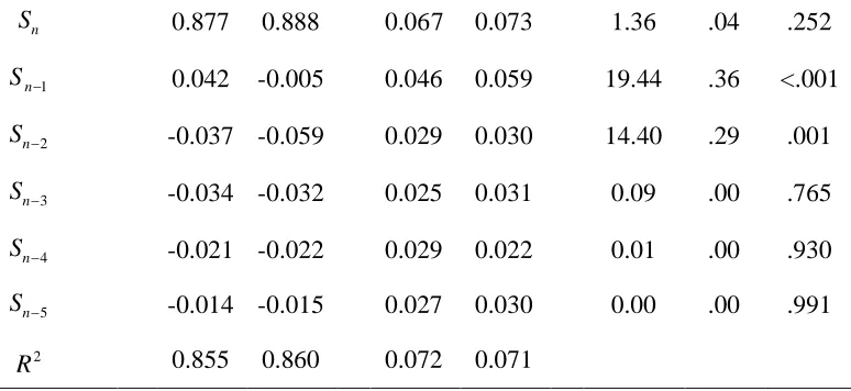
Table 1. Regression coefficients for the only regression (Equation 1) and stimulus-response regression (Equation 2) from Experiment 1.
Predictor or 2
R Mean SD F(1,35)
2
p
K p
Short Long Short Long
Stimulus-only regression (Equation 1)
n
S 0.877 0.888 0.067 0.073 1.36 .04 .252
1
n
S 0.042 -0.005 0.046 0.059 19.44 .36 <.001
2
n
S -0.037 -0.059 0.029 0.030 14.40 .29 .001
3
n
S -0.034 -0.032 0.025 0.031 0.09 .00 .765
4
n
S -0.021 -0.022 0.029 0.022 0.01 .00 .930
5
n
S -0.014 -0.015 0.027 0.030 0.00 .00 .991
2
R 0.855 0.860 0.072 0.071
Stimulus-response regression (Equation 2)
n
S 0.877 0.887 0.066 0.073 1.24 .03 .274
1
n
S 0.009 -0.047 0.078 0.110 11.29 .24 .002
1
n
R 0.040 0.049 0.081 0.082 0.34 .01 .565
2
n
S -0.032 -0.066 0.067 0.071 5.30 .13 .027
2
n
R -0.008 0.015 0.062 0.072 2.22 .06 .145
2
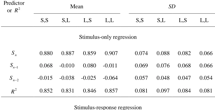
Table 2. Regression coefficients for the stimulus-only (Equation 1) and stimulus-response regression (Equation 2) analyses for Experiment 2.
Predictor
or R2 Mean SD
S,S S,L L,S L,L S,S S,L L,S L,L
Stimulus-only regression
n
S 0.880 0.887 0.859 0.907 0.074 0.088 0.082 0.066
1
n
S 0.068 -0.010 0.080 -0.011 0.069 0.076 0.068 0.066
2
n
S -0.015 -0.038 -0.025 -0.064 0.057 0.048 0.047 0.054
2
R 0.852 0.831 0.846 0.857 0.081 0.097 0.084 0.081
Stimulus-response regression
n
S 0.885 0.890 0.864 0.908 0.074 0.088 0.079 0.068
1
n
S 0.030 -0.048 0.029 -0.080 0.113 0.155 0.128 0.141
1
n
R 0.043 0.046 0.059 0.079 0.107 0.148 0.115 0.133
2
n
S -0.033 -0.042 -0.048 -0.077 0.109 0.111 0.119 0.116
2
n
R 0.016 0.000 0.037 0.015 0.121 0.123 0.120 0.107
2
R 0.861 0.836 0.857 0.863 0.074 0.094 0.076 0.082
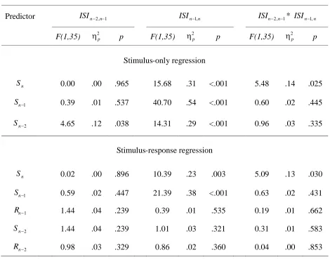
Table 3. ANOVA results for stimulus-only (Equation 1) and stimulus-response regression (Equation 2) coefficient from Experiment 2.
Predictor ISIn2,n1 ISIn1,n ISIn2,n1* ISIn1,n
F(1,35) K2p p F(1,35)
2
p
K p F(1,35) K2p p
Stimulus-only regression
n
S 0.00 .00 .965 15.68 .31 <.001 5.48 .14 .025
1
n
S 0.39 .01 .537 40.70 .54 <.001 0.60 .02 .445
2
n
S 4.65 .12 .038 14.31 .29 <.001 0.96 .03 .335
Stimulus-response regression
n
S 0.02 .00 .896 10.39 .23 .003 5.09 .13 .030
1
n
S 0.59 .02 .447 21.39 .38 <.001 0.63 .02 .431
1
n
R 1.44 .04 .239 0.39 .01 .535 0.19 .01 .662
2
n
S 1.44 .04 .239 1.01 .03 .321 0.31 .01 .583
2
n
Figure Legends
Figure 1. Impulse plots for Experiment 1.